DONALD ALLEN WIDEN
B.S., Bowling Green State University (1960)
SUBMITTED IN PARTIAL FULFILLMENT OF THE REQUIREMENT FOR THE
DEGREES OF MASTER OF SCIENCE
at the
MASSACHUSETTS INSTITUTE OF TECHNOLOGY August 22, 1966
Signature of Author ... ,...
Departments of Aeronautics and Astronautics
I --- *
~-&.
4 I Or=Cr ... f- . ...
-- imarvisgor
Accepted by
Cha an, epartmental Committee on Graduate Students
OF
TECHN
01,
*SEP 19 968
Zoo
I u
L
38
CONCENTRATION OF OZONE IN SURFACE AIR OVER GREATER BOSTON
by
DONALD ALLEN WIDEN
Submitted to the Departments of Aeronautics and Astronautics and of Meteorology on August 22, 1966 in partial fulfillment of the
requirements for the degrees of Master of Science.
ABSTRACT
Surface ozone concentrations were measured in the Greater Boston area from November, 1964 to December, 1965. Ozone was monitored continuosly using a Mast microcoulombmetric sensor. A chromium tri-oxide filter was fitted to the air inlet of the sensor in order to remove negatively interfering sulphur dioxide. Daily ozone concentra-tions near the surface varied from somewhat greater than 10 to less than 1 pphm by volume. The highest concentrations occurred in late spring while the lowest concentrations occurred in the winter. Such a seasonal variation would be expected if the ozone had arrived in the troposphere from the lower stratosphere. The concentration of ozone during the spring and early summer showed a much greater variability from day to day than was exhibited during the fall and winter months.
Thesis Supervisor: Reginald E. Newell
I. INTRODUCTION ... ... 1
II. PROPERTIES OF OZONE ... . ... . 3
III. OZONE IN THE UPPER ATMOSPHERE ... . . 4
Source of Ozone ..0000000000000.000.000... 4
Distribution and Variation ... ... 00000 7 Seasonal and Latitudinal .000000... 7
Vertical ... ... 7
Transport Properties... 12
IV. OZONE NEAR THE GROUND ... 000000 15 Sources of Tropospheric Ozone ... 15
Distribution and Variation ... 18
V. INSTRUMENTATION ... 23
Sensor and Recorder ...0... 23
Sulfur Dioxide Removing Filter ... 24
VI. SAMPLING SITES ... 27
VII. DISCUSSION OF OBSERVATIONS ... 28
Sources of Error ... 28
Ozone in the Boston-Cambridge Complex ... 30
Seasonal Variation ... 30
Day to Day Variation ... 33
Diurnal Variation ... 38
Thunderstorm Correlation ... 41
( -Activity Correlation ... 41
Sea Breeze Correlation ... 42
Case Studies ..0000000000000000000... . 44
VIII. RECOMMENDATIONS ... 48
BIBLIOGRAPHY ... 49
APPENDIX A .. o... 54
LIST OF FIGURES
Page
Figure 1. Mean distribution of total ozone... 8
" 2. Annual variation of total ozone... 9
" 3. Mean ozone density for March-April 1963 .... 10
" 4. Annual variation of ozone as a function of altitude ... 11
" 5. Possible mechanisms for ozone transfer 14 " 6. Yearly variations of ozone ...- 19
" . 7. Diurnal variation of ozone ... * 21
" 8. Seasonal variation of ozone at Boston ... 31
9a. Daily variation of ozone ... 34
9b. " "...- . .-. 35
" 10. Diurnal variation of ozone ... 39
" 11. Mean diurnal variation ... 40
12. Monthly variation of maximum surface ozone and (*-activity ... 43
" 13. Diurnal variation of wind speed, temperature, and ozone .. 0...0...0... 45
" 14. Diurnal .variation of wind speed, temperature, and ozone ... ... - 46
I. INTRODUCTION
The National Academy of Sciences National Research Council convened an International Planning Conference on Atmospheric Ozone in 1964 to review the observational and research needs for the study of ozone. They found that it is necessary to plan for an extended network of observations so that pertinent and useful data can be obtained. Prior to this, Junge, in his 1962 study of the global ozone budget, concluded that further systematic measurements of surface ozone at a number of sites over the globe would be of great value in consideration of stratospheric-tropospheric exchange processes. Such studies could provide information about where and when stratospheric air reaches the lower troposphere. Combined with ozone sounding data such as that gathered by Mr. W.S. Hering and his group at the Air Force Cambridge Research Labor-atories, it is not unreasonable to hope that eventually the quantity of stratospheric air passing into the troposphere can be estimated.
An objection often raised to Junge's proposed network of surface ozone stations is that measurements made near a city can be contaminated with ozone produced locally by the action of sunlight on automobile and industrial
exhausts. There is some direct evidence of such production in the controlled experiments of Ripperton (1965) and in the existence of high ozone values in the polluted air of a relatively unventilated city like Los Angeles. This may account for the fact that the only surface ozone measurements added to the literature since Junge's paper .are apparently those from the Antarctic reported by Aldaz (1965) and those from Alaska reported by Kelley (1966). Thus, the question of the feasibility of the network suggested by Junge has not really been decided. In view of the interest in the general circulation of ozone in the atmosphere and its possible use as a tracer of the vertical
-2-transfer of energy from the troposphere to the stratosphere (Newell 1961, 1964), it was decided to monitor surface ozone in the relatively well ventilated region of Greater Boston.
II. PROPERTIES OF OZONE
The molecule of Ozone, 03, consists of three atoms of oxygen. Its density is 2.144 gram/liter (00C, 760 mm). This pale bluish gas is formed when an electrical discharge passes through oxygen. Thus ozone is produced in the atmosphere during electrical storms and has a charac-teristic "electrical odor". Ozone will liquify into a blue black liquid at -112
0C
and will solidify at -251.4 C. Its chemical properties are similar to those of oxygen, but it reacts more easily. Silver, for example, (which remains bright and shining for years in oxygen) will quickly become covered with a brown film of silver oxide when exposed to ozone.
-4-III. OZONE IN THE UPPER ATMOSPHERE
A. The Source of Ozone
Ozone formation in the atmosphere is not completely understood. How-ever, it is widely accepted that practically all ozone found in the upper atmosphere is formed by the photochemical action of ultraviolet light on oxygen. Since ozone is also destroyed by photochemical processes, the concentrations of ozone are determined by an equilibrium condition between formation and destruction. Of the number of reactions in which ozone is involved, only four are thought to be important for quantitative consider-ations (Junge, 1963):
02 + hv -+, 20 (- 2400
A)
(1)02 + 0 + M- 03 + M (2)
03 + hv -+ 0 + 0 (d 11.,000A) (3)
03 + 0 - 202 (4)
Equations (1) and (2) lead to the formation of atomic oxygen and ozone. The M in equation (2) represents a neutral molecule which is, for all practical purposes, oxygen or nitrogen. Thus, radiation in the Schumann-Runge (1760 - 1925
A)
and Herzberg bands produces ozone. The destruction process is controlled by equations (3) and (4), in which ozone is destroyed by the absorption of energy at wavelengths less than 11,000 A. These low energy wavelengths contain the ultraviolet Hartley (2000 - 3200A)
and the visible Chappius (4500 - 7000A)
bands. The Hartley bands are most impor-tant for ozone photolysis.The processes of formation and destruction are not separate but are carried on concurrently in the same volume of space and at the same time. Thus, an expression for the equilibrium concentration of ozone in terms of reaction rate constants, absorption coefficients, quantum yields, and intensity of solar radiation can be derived. (Craig, 1950; Johnson, 1954; Junge, 1963). Because the quantities involved depend on the wavelength of the radiation as well as on altitude, the calculation of the vertical and latitudinal distribution of ozone is very time consuming.
The photochemical theory predicts the maximum amounts of ozone in the layer between twenty and thirty km. It also predicts that the seasonal maximum should occur in June with the minimum occurring in December. The latitudinal maximum would be found at the Equator for all seasons with decreasing amounts predicted as the Poles are approached.
As will be seen in the following section, observations of the vertical distribution of ozone confirm the presence of the predicted maximum layer. However, observations of the horizontal distribution indicate an increase
in the total amount of ozone with latitude. The higher values in middle and high latitudes are found during the late winter and spring rather than in the summer as the theory predicts. Besides this, the numerical value of the amount of ozone predicted is too low.
Nicolet (Newell, 1963) found that the time necessary to reach 50% of the photochemical equilibrium concentration, after a disturbance in which the ozone content of an air parcel is entirely removed, is thirty minutes, three days and seven months, for heights of 50, 30 and 20 km respectively
-6-for the overhead sun and 90 minutes, one month and 12 years -6-for the sun at the horizon. These characteristic times are also discussed by
Hesstvedt (1963) and Leovy (1964). As a result of the calculation of characteristic times, it is obvious that the ozone concentration below 30 km is not influenced directly by the sun. Thus theory and observation can be reconciled if atmospheric circulations are postulated which trans-port ozone from low to high latitudes or downwards out of the photochemical equilibrium regions in middle and high latitudes. With such circulations, the photochemical theory gives a very satisfactory explanation of the ozone problem.
B. Distribution and Variation of Ozone
1. Seasonal and latitudinal variation
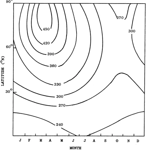
Figure 1 shows the mean distribution of total ozone as a function of month and latitude. It can be seen that the amount of total ozone is a maximum at high latitudes and a minimum at the Equator. The maximum at high latitudes occurs during the late winter and early spring and the minimum occurs during the autumn months. The amplitude of the annual variation, Fig. 2, has a maximum towards the Pole and decreases toward the Equator. The pronounced spring maximum and fall minimum at high latitudes are also clearly shown in the latter figure.
2. Vertical distribution
Measurements of the vertical distribution of ozone indicate that the concentration of ozone increases with height. The main maximum occurs between 20 and 25 km. However, a secondary maximum may be found between 13
and 27 km depending on the season and latitude. Above the main maximum, the concentration then falls. The vertical distribution is shown in Fig. 3.
Dutsch (Taba, 1961) noted that the height of the maximum level changes from season to season. The maximum level is the lowest in the early spring, when the ozone amount has its highest value and it reaches its greatest altitude in late summer.
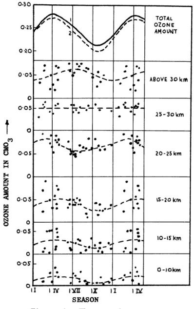
Figure 4 depicts "the seasonal variation of ozone concentration for different altitudes, based on balloon data (Paetzold, 1955). It de-monstrates that the total ozone measured at the ground is a rather complex net effect of the seasonal variations at different altitudes. The 15-20 km
-8-900 70 450 300 600 420 390
z
0 360 330 30 3 300 3270 240 J F M A M J J A S 0 N D MONTHFigure 1. Mean distribution of total ozone as a function of mogth and latitude. The isopleths give total ozone in 10 atm-cm (STP cm) on the Vigroux scale. (Godson, 1960).
iga-mmeff-JAN. MAR. MAY JUL. SEP. NOV. JAN.
Figure 2. Annual Variation of Total Ozone (Brewer, 1960) CM OF
OZONE S.T.P.
200 tooo 50010 0 Soo 400 30 30-28 26 24 22 20 18-16 14 12- 10-8 6 4 2 0 90
N
.1 -. so 80 70 60 50 40LATITUDE (DEGREES NORTH)
-3 Figure 3. Mean Ozone Density (A g m ) for
(Hering and Borden, 1964).
20 10 March-April 1963 500 1200 soo 30 28 26 24 22 20 18 16 14 12 10 8 6 4 2 0
0:30 ' * < * *', ., .,.-*' oe * --. 0.05 20-25 km z 1-4 E-4 0 o 6. , 0-05 - .. - -% .* , - - 5-20 km * * % ... --- . 6 Z 0 *e .0 o --0 0-0 00 0-o5 - -* * . - 10-15km o ---- -- *-* 0 0-0s0 0--okm aI I I - -I* I SEASON
Figure 4. The annual variation of ozone as a function of altitude. Curve 1 is the total amount of ozone from balloon data and curve 2 represents the same from Dobson's measurements in Arosa (Paetzold,
-12-layers show the familiar spring maximum, which is somewhat delayed in the troposphere. The 25-30 km layer does not show any systematic variation at all and above 30 km the seasonal variation is in phase with the zenith distance of the sun, as is to be expected from the photochemical ozone theory."
C. Transport Properties
In order to reconcile the discrepancies between theory and obser-vation, a circulation which transports ozone from low to high latitudes or downward out of the photochemical source region is necessary. Since the majority of atmospheric ozone is located in the 20 to 30 km layer, the north-ward transport of ozone must be supplied by the general circulation of the lower stratosphere. The stratospheric circulation which best fits energy and momentum considerations is one in which ozone is transported northward in middle latitudes by quasi-horizontal eddies (Newell, 1961). Mean merid-ional motions and standing eddies appear to play a relatively minor role in the transport.
Newell (1964) shows that the average covariance between total ozone and meridional wind in the lower stratosphere (100 mb) is overall positive between 600 and 900 indicating that northward moving parcels contain more ozone on the average than southward moving parcels of air. Also, the eddy processes are more active in the winter and spring than in the summer and autumn; hence the observed spring maximum is explained.
From the lower stratosphere there is a steady downward flux of ozone (Reed, 1953 and Dutsch, 1959) into the troposphere where it is
destroyed in large quantities by chemical, photochemical and catalytic processes. The process of ozone exchange between the stratosphere and troposphere is still not thoroughly understood. However, possible ex-change mechanisms have been discussed by Danielson (1959, 1964), Brewer
(1960), Staley (1960), Newell (1963a) and others. These authors indicate that the transfer apparently occurs in the vicinity of the jet stream, in frontal zones and perhaps also directly across the tropopause region. Brewer lists four possible exchange mechanisms:
1. There may be a continuation across the tropopause of the slow nonadiabatic descent which is presumed to have brought the ozone down to the tropopause. This is shown by arrows A of Fig. 5.
2. If the tropopause slopes relative to the isentropic surfaces, motion along an isentropic surface can extract ozone from the stratosphere. (arrows B).
3. Exchange can occur along isentropic surfaces which pass through the subtropical jet of the temperate regions.
(arrow C).
4. There is also the possibility of a circulation through the lower stratosphere as shown by arrow D.
-14-20 I v'WM1~ 4- *C ___. EQUATOR POLE
Figure 5. Possible Mechanisms for the transfer of ozone from the Temperate Stratosphere into the Troposphere (Brewer, 1960).
TROPOPAUSE BA
IV. OZONE NEAR THE GROUND
A. Sources of Tropospheric Ozone
There is still speculation as to the origin of ozone found near the surface. Regener, in 1941, was the first to advance the thesis that tro-pospheric ozone originates in the stratosphere. He proposed that strato-spheric ozone is transported downward into the troposphere by the various air exchange mechanisms operating in the vicinity of the tropopause.
During its downward journey through the troposphere the ozone is chemically destroyed in clouds, by gaseous and particulate trace substances and pri-marily by contact with the earth's surface.
Another source of tropospheric ozone is the polluted layer of surface air in the urban areas of the world. The production and destruction of ozone in such polluted layers is primarily governed by the following re-actions (Leighton and Perkins, 1958):
NO + hv -+ NO + 0 (3100 A < 3700 A) (5)
2
0 + 02 + M -- 03 + M (2)
03 + hv -.. 0 + 0 (3)
NO + 03 -- NO2 + 0 (6)
The M in equation (2) represents any particle capable of absorbing energy released by the reaction. If no M were present, the ozone would be unstable and would quickly dissociate. Since solar radiation of wavelength less than 2900
A
is absorbed by the upper atmosphere, the wavelength of the quantum of energy involved in equation (3) is restricted to 2900 to 3200A
in the ultraviolet Hartley bands plus the visible Chappins bands.
-16-The presence of other constituents in the polluted air may affect the rate at which the above reactions occur, even though the constituents are not immediately involved. For example, Schuck and Doyle (1959) report that the rate of ozone production is increased in the presence of olefins and decreased in the presence of paraffins. Some types of olefins not only increase the rate of production, but also tend to support high
con-centrations of ozone.
Of the constituents directly involved, the oxides of nitrogen are perhaps the most important. The nitrogen dioxide found in the lower
atmo-sphere is a by-product of high temperature combustion processes such as those found in the internal combustion engine and in industrial furnaces. The chemical processes involved in such combustion processes are discussed
in detail by Dickinson (1961) and Leighton and Perkins. Kawamura (1964) found that the concentration of nitrogen dioxide in Tokyo showed a marked diurnal variation with a maximum three hours after sunrise and another maximum two hours after sunset. A similar result was found by Dickinson
(1961) in the Los Angeles area. To show the importance of oxides of nitrogen in the formation of surface ozone, Kawamura (1965), assuming
a photochemical equilibrium with regard to the concentration of NO2 in polluted air, obtained the following equation
k2 (NO) (03) (7)
(NO2 Ok a x k1(03)
where k1 and k2 are the rates of reactions of ozone respectively with NO2 and NO; k a, the rate of absorption of ultraviolet solar radiation by NO2; 0 , the quantum yield of NO2 photolysis. From his results of
simultaneously measuring the concentration of ozone, nitrogen dioxide, and nitric oxide, he concluded that the concentration of ozone during most of the daylight hours is controlled by the presence of oxides of nitrogen. Vassy (1963) found the ozone concentration of Paris to be approximately one-tenth of the concentration measured in Los Angeles during comparable conditions. He attributed most of the difference to the smaller number of automobiles in Paris. In a similar comparison between London and Los Angeles, the ozone concentration ratios were in the same proportion as the engine cylinder ratios.
Ozone is also produced when an electric discharge dissociates mole-cular oxygen into atomic oxygen; the atomic oxygen then combines with molecular oxygen to produce ozone. In the troposphere electric discharges are produced mainly by lighting in thunderstorms; but they may also origin-ate from power lines.
In spite of the fact that most observers agree that ozone is produced in detectable quantities by electric discharge in the troposphere, there is some question as to whether this increase is detectable at the surface. Vassy (1954) found, while measuring surface ozone in Paris, that there is
an abrupt increase in the concentration of surface ozone during thunder-storms. The abrupt increase was found to preceed the first discharge by three and one-half hours on the average. Over a period of two years Dmitriyev (1965) made observations of 47 cases, in 37 of which a sharp increase of ozone was followed by thunder showers at the place where the concentrations were measured. Kroening and Ney (1962) estimate that the amount of ozone produced by lightning is of the same order of magnitude
-18-as that produced by solar ultraviolet light. Junge (1963), in contrast to this estimate, points out that there is no evidence of tropospheric ozone sources, except for polluted areas, e.g. Los Angeles. Gluckauf (1944) and Dobson (Gluckauf, 1951) support Junge's thinking in that they found no abrupt increase in surface ozone prior to the thunderstorm activity which they studied.
There has been speculation (Went, 1960) that some ozone is formed by photochemical secondary reactions in the lower atmosphere even in relatively unpollued air. A study by McKee (1961) in Greenland supports this hypothesis. Doubtless, there are other sources of tropospheric ozone; but none of them would contribute significantly to the ozone budget, and thus they will not be mentioned here.
B. Distribution and Variation
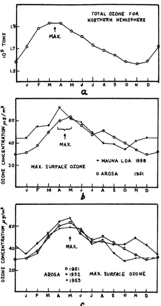
A survey of representative tropospheric ozone data (Junge, 1962) revealed that within the northern hemisphere the data exhibited a uniform seasonal variation, the phase of which was delayed about two months with respect to the injection of stratospheric ozone into the troposphere. This yearly variation is not quite symmetrical; the spring maximum being sharper and better defined than the broad winter minimum. This is seen in Fig. 6, which depicts the yearly variation of ozone at Mauna Loa, Hawaii and Arosa, Switzerland. A similar variation has also been found by Kelley (1966) who made measurements at Barrow, Alaska during 1965. Southern hemisphere observations made in the Antarctica by Wexler, et. al.
e~60 V 4 0 '-' 20 hi Z 0 P4 0 F. - MAX, + MAUNA LOA 1956 MAX. SURFACE OZONE
0 AROSA I93i
I i I i i I 1
J' F M A M JI J A SO o~ D
Figure 6. Yearly variations of ozone. a, Total stratospheric ozone burden for the northern hemisphere.
b, Comparison of monthly average values of daily maximum ozone concentrations at ground level.
c, Comparison of 3 years of monthly average values of daily maximum ozone
concentration at ground level (Junge, 1962). rOTAL OZONE FOR
WORTHERN WEMISPIERE
MAX,
Ij F M A M J J A 5 o N D CL
-20-Day-to-day variations superimposed on the seasonal trend have also been observed. Regener (1954a) found that day-to-day variations of the average daily concentrations seem to be small, except when sudden meteor-ological changes occur. This observation is supported by Kelley who found that daily fluctuations show a greater variability during early winter and spring than in summer and fall. Such short term fluctuations may be caused by destruction of ozone near the ground, by a somewhat
different history or "ozone age" of the different air masses or by changes in the transport mechanism which operates to bring ozone rich air from the stratosphere to the ground. In spite of these fluctuations, Junge (1962) found that the upper limits of the range of ozone concentra-tions are rather uniform. Thus he concluded that the representative ozone concentrations within the troposphere do not vary too much with time and space. He also noted an agreement between Mauna Loa and the continental sites which would indicate that the average ozone destruc-tion rate over oceans cannot be too different than that over continents.
In addition to the seasonal and day-to-day fluctuations a marked diurnal variation of surface ozone occurs in relatively unpolluted air during calm weather. This diurnal variation is characterized by a broad minimum at night, a rapid rise in the morning after sunrise, and a sharp maximum near noon. The typical diurnal curve shown in Fig. 7
is based on 1961 data taken at Port Burwell, Ontario (Cole and Katz, 1966). This figure shows a comparison of a typical low ozone day on August 20 with August 18, a day of maximum ozone occurrence. The mean hourly
0 4 8 12 16 20 24 HRS. Figure 7. Diurnal variation of ozone.
-22-values of ozone concentration for July through September 1961 are also shown. The typical diurnal variation indicates a characteristic photo-chemical pattern that follows the solar cycle of light and darkness in
a remarkable manner. It is possible that the diurnal variation is caused solely by the photochemical production of ozone at or near the ground. Then again it could be produced solely by vertical descent of ozone through turbulent mixing caused by solar heating. The cause of
the diurnal variation is possibly a combination of these two effects.
The profile shown in Fig. 7 however, is not characteristic of mountain sites where the ozone concentrations, measured by Ehmert and Ehmert (Junge, 1963), Regener (1954b) and Price and Pales (1959), show practically no diurnal variation. Nor is it characteristic of polluted
areas such as the Los Angeles Basin. In addition, no marked diurnal variation is found when the surface winds are strong (greater than
10 knots) and gusty. In this case, the broad nightly minimum is absent because turbulent mixing prevents the layers of air near the ground from
becoming stagnant, thus preventing at least some of the ozone destruction which takes place when stagnant air comes in contact with the ground.
V. INSTRUMENTATION
A. Mast Ozone Sensor
1. Theory of operation
The Mast ozone meter utilizes the well-known oxidation reduction of potassium iodide which is contained in the sensing solution. Ozone in the air sample reacts with the sensing solution to liberate iodine on the cathode portion of an electrical support. Measurement of the iodine is accomplished by a microcoulomb cell developed by Brewer (Brewer and Milford, 1960). The basic reaction is:
03 + 2 KI + H2-+ 02 + 12 + 2 KOH (8) At the cathode, a thin layer of hydrogen gas is produced by a polarization current:
2e + 2H -+ H2 (9)
When a potential of approximately 0.25 volts is applied externally to the electrodes, the hydrogen layer builds to its maximum and the polarization current cases to flow. The free iodine formed in the oxidation of the potassium iodide immediately reacts with the hydrogen as follows:
H + 1 -+ 2 HI (10)
2 2
The removal of the hydrogen from the cathode causes an additional current to flow to reestablish the hydrogen layer at the cathode. This repolari-zation current causes two electrons to flow in the external circuit for every ozone molecule reacting in the sensor. Thus, the current, or rate
of electron flow, is a linear function of the mass per unit time of the ozone entering the sensor.
-24-2. Operational characteristics
The sensor can be used as a direct reading device or in connection with a strip chart recorder which is calibrated in parts per hundred million by volume (pphmv) when the air flow rate is 140 ml/min at STP. The air-sample flow, including the direction and turbulence of the air-sample as it enters the sensor has been demonstrated (Mast and Saunders, 1962) to be relatively uncritical for a constant flow rate of 140 ml/min. However, Cherniack and Bryan (1965) indicate that the Sensor is critically sensitive to unevenness in the flow rate.
A distinct advantage of this instrument is that the exact composi-tion of the solucomposi-tion is not critical. Thus, there are no critical measure-ments or standardizations required in the preparation of the solution. Also, the solutions are quite stable for months.
A more complete description of the relative merits and limitations of the Mast Ozone Recorder have been well noted by Potter and Duckworth (1965) and by Mast and Saunders (1962). Studies by Cherniack and Bryan (1965) and by Hering and Dutsch (1965), compare the Mast coulometric system with other types of ozone detectors which are being used for atmo-spheric air sampling today.
B. Filter Used to Remove Sulfur Dioxide
It is a well documented fact (Wartburg and Saltzman, 1963, Kawamura 1964, Ripperton 1965, and Cherniack and Bryan, 1965) that sulfur dioxide produces serious negative interference in the electrochemical method of the determination of atmospheric ozone. Saltzman and Wartburg (1964),
Ripperton (1965) and Cherniack and Bryan (1965) have suggested simple methods of removing sulfur dioxide from the sample air strem (with little or no loss of ozone) in order to improve the accuracy of iodometric measuring devices such as the Mast instrument.
Used in this study was a filter made of fiber-glass paper on which was dried a solution of chronium trioxide acidified with sulfuric acid. The method of preparation of Saltzman and Wartburg's filter (Brandli, 1965) is as follows:
Prepare a 10 ml solution containing .83 - 1.66 grams of chromium trioxide and .46 - .93 cc concentrated sulphuric acid. Drop solu-tion (with eyedropper) onto 6 sq. in. of glass fiber filter paper; dry paper in oven at 800C for one hour or until paper turns pink,
(in this case, it happens in approximately one half hour). Now, cut dried filter paper into 1/4 by 1/2 inch pieces and fold the pieces into V shapes. Place the folded paper into 100 mm Schwarz
IJ
tube (glass). (A 100 mm straight polyethelene tube was used here). The paper (pie shaped because circular filter paper was used, 1 inch diameter) was folded to prevent nesting together when packed in the tube. The final product resembled a large cigarette type filter and acted in essentially the same manner. Conditioning of the filter and also ensuring against any blocking of the air in-take flow was accomplished by drawing laboratory air through the filter with the aid of a small vacuum pump. The theory of this filter technique is based on the fact that the chromium trioxide
-26-is an excellent oxidizing agent; thus the sulfur dioxide -26-is oxidized to SO3 (highly hygroscopic) which then clings to the glass fiber filter paper. Filters were used for approx-imately thirty days before being replaced, as was suggested by Saltzman and Wartburg.
VI. SAMPLING SITES
Ozone data collected for this study was taken at three different locations in the Boston-Cambridge complex. The majority of data was collected from the roof of the MIT Green Center for Earth Sciences, at a height of 100 meters. On the roof, the sensor was located some 25 meters west of the building's air conditioning unit which operated continuously from May to September. During December 1964 and January 1965, air was sampled in Roslindale, approximately fifteen kilometers southwest of the MIT campus. The instrument was placed in a second floor room eight meters above ground with the inlet tube protruding from the window. For February, 1965, the sensor was moved to Braintree, some twenty-five kilometers south-southwest of the campus. Here the window used was only one meter above the ground.
-28-VII. DISCUSSION OF OBSERVATIONS
A. Sources of Error
When measuring ozone with the Mast electrochemical instrument, one should be aware of possible interference caused by oxidants other than ozone and reducing agents. Of the possible interfering agents, sulfur dioxide, which produces a negative interference of nearly 100%, is the most important. In order to avoid such negative effects, the instrument used in this study was fitted with a chromium trioxide filter (Wartburg
and Saltzman, 1963) which is described in a previous section of this
thesis. The use of this filter however, is not recommended in areas where the ratio NO/SO2 is large. In such areas, the chromium trioxide in the filter will oxidize NO to NO2 and the nitrogen dioxide then produces a positive interference. Also, the authors report that when the filter is exposed to air at higher than 90% relative humidity, ozone recovery drops to 90%; but as the papers dry, ozone recovery comes back to 100%.
Another interfering agent found in most polluted atmospheres is nitrogen dioxide, which as previously stated will produce a positive interference. In a controlled nitrogen dioxide interference test with the Mast Ozone Detector, Cherniack and Bryan found a positive interference of 10%. However, during the atmospheric sampling portion of their study they found the value of NO2 too low to cause appreciable interference.
The average concentration of NO2 in the Boston, Mass. atmosphere was found to be 6 pphm (Tabor and Golden, 1965). This value is an average of 65 samples taken over a two year period (1961-1963) by the National
Gas Sampling Network. The maximum concentration found was 13 pphm. Using the 10% value of the positive interference, the maximum error induced by NO2 might be expected to be on the order of 1.3 pphm while the average
error would be approximately 0.6 pphm. Thus the ozone concentrations given in this study might be expected to average about 0.6 pphm higher than the actual ozone content. The disturbing effects due to the presence of other interfering agents such as the nitrate ion (NO3-), chlorine, organic perox-ides, etc. may be assumed to be negligible.
Cherniack and Bryan (1965) point out that the Mast analyzer is critically sensitive to air flow but much less sensitive to reagent flow. In order to
avoid possible errors the flow rate was checked and adjusted if necessary every three months. During the period of operation however, the instrument was not calibrated. Thus it is possible that the sensitivity of the micro-coulomb detector could have decreased with age as was reported by Kelley
(1966). Interference by nearby radio transmitters can cause spurious chart readings (Potter and Duckworth, 1965). Such interference is tolerable because the "spikes" are infrequent and easily spotted.
Because ozone is a highly reactive compound, the intake tubing should be as short as possible. A glass intake tube may cause a destruction of ozone from the wall effect (Kawamura, 1964). In this study, a 30 cm poly-ethelene and teflon tube was used for the air inlet. For this reason there should be no significant loss of ozone due to the so-called wall-effect in this study.
-30-A change in height of the sensor above the ground can produce a large change in the ozone concentration. This is especially true when the weather conditions are stagnant, in which case the vertical ozone gradient is large. Since the height of the sensor in this study varied from one meter to 100 meters above the ground, care should be taken when making a comparison of
the ozone concentrations obtained at the different sites.
In order to correct for ambient conditions and thus get a more accurate reading, the instrument values should be multiplied by
p(ambient) T(standard) p(Standard) T(Ambient)
This correction factor was not applied to the data contained in this thesis. The uncertainty or accuracy of the instrument is reported to be 1 ppbv (parts per billion by volume) which is approximately the limit to which the graph on the recorder can be used.
B. Ozone in the Boston-Cambridge Complex 1. Seasonal variation
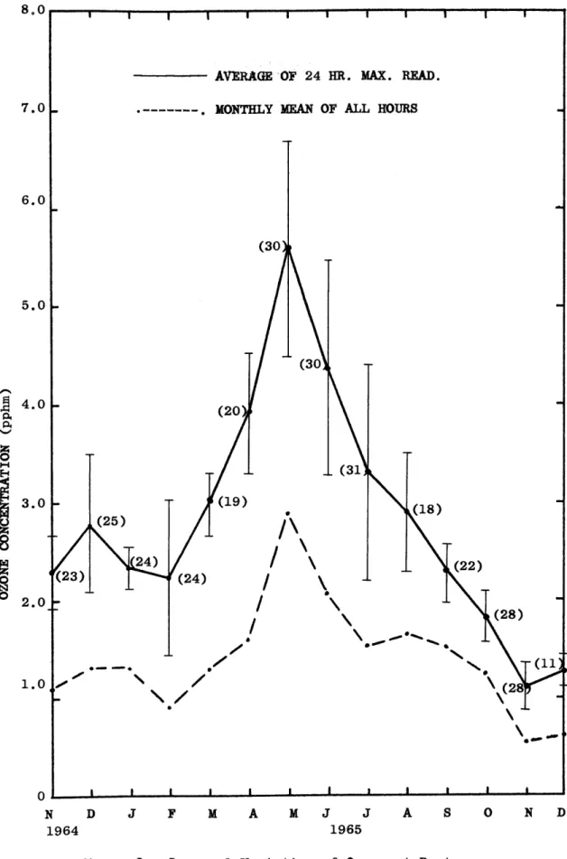
Figure 8 shows a plot of the monthly means, which were computed by averaging one hour means for the entire month. Also plotted are the average daily maximum values, which should give a more representative value for the
lower troposphere since the effect of ozone destruction near the ground is minimized. The vertical line segments represent the standard deviation, while the number in parenthesis indicates the number of days included in the sample. The maxima usually occurred early in the afternoon. Ozone
AVERAGE OF 24 HR. MAX. READ.
7.0 .---. MONTHLY MEAN OF ALL HOURS
6.0 (30 5.0 (30 '0 ~ (20 0 (31 3.0 (25) (19) ( 18) (25) 24)
\
(22) (23) (24)-(28)
.. .-. 4" (11 1.0 (28 0 0 I I I I I , I a p N D J F M A M J J A S 0 N D 1964 1965
-32-concentrations are a maximum in late spring as would be expected if the ozone had arrived in the troposphere from the lower stratosphere. The maximum in
total ozone which usually occurs in March or April is the result of a build-up of ozone in the lower stratosphere. The maximum of surface ozone was
found in this study to occur in May. This time delay of one to two months may be the net result of the rate of stratospheric-tropospheric mass exchange
plus the rate of dispersion of ozone in the troposphere. In addition, the rate of ozone loss to tropospheric aerosols, to the surface and in reactions with the oxides of nitrogen (Kawamura, 1965) may also be factors that enter
into this time delay. Without a network of stations it is practically impossible to sort them out. Likewise, the minimum in November, 1965 is about one month later than the average minimum in total ozone. The general form of the annual variation is the same as that reported for Arosa, as seen in Fig. 6. However, the amplitude of the variation is somewhat greater; but until records for several years have been accumulated it is not possible to attach any significance to this finding. Instrument response, presence of the filter, and year to year variations are all factors that may be involved. This figure does contradict the conclusions of Ripperton (1965) and Mc Kee
(1961) who support the theory that tropospheric ozone is primarily formed photochemically near the ground. If their conclusion were correct, Fig. 8 would show a maximum in the summer corresponding to the maximum solar heating.
2. Day to Day Variations
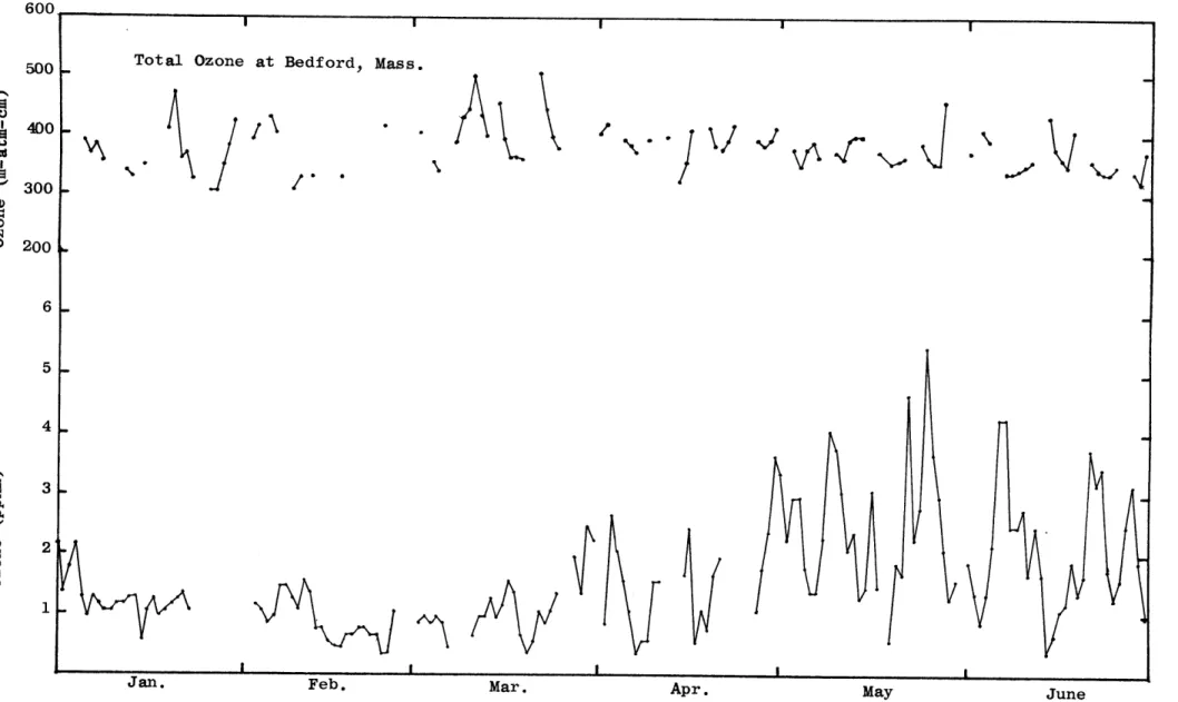
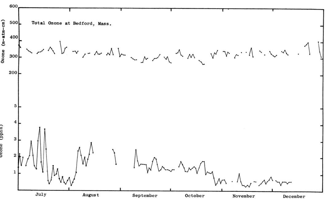
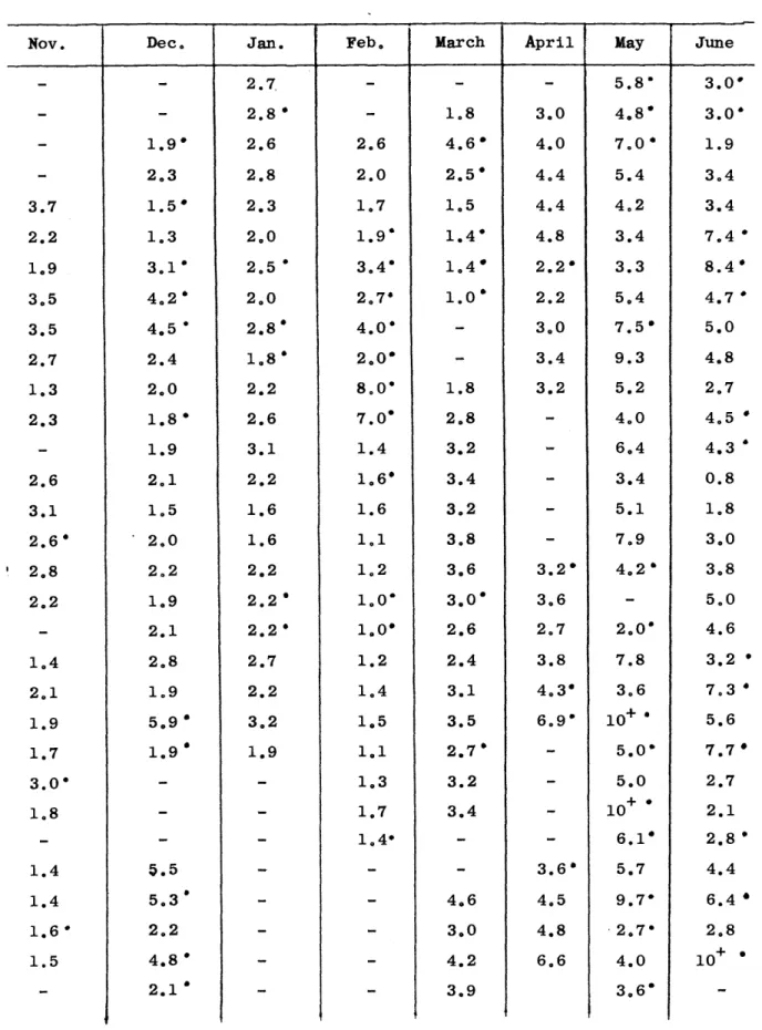
Daily fluctuations in average concentrations of surface ozone show a much greater variability during the spring and early summer than in the fall and winter (Figs. 9a and 9b). Kelley (1966) reported similar fluctua-tions in the atmospheric ozone content at Barrow, Alaska. He also found that the large fluctuations superimposed on the seasonal trend are almost always correlated with the passage of frontal systems. A similar correlation between large ozone changes and frontal systems was found in this study. Also shown in Figs. 9a and 9b is the variation of total ozone over Bedford, Massachusetts. This data was kindly supplied to the author by Mr. W.S. Hering and his group at the Air Force Cambridge Research Laboratories. A comparison of total ozone and surface ozone shows that the variation of ozone in the total column is similar to the variation of surface ozone. The maximum of total ozone occurs during March while the minimum occurs during September. Since ozone measured at or near the surface is affected by the sink at the surface and by the local surface circulation, the daily maximum concentra-tions of surface ozone are included in Table 1.
600.
500
400
300
200
o 300 . 200-Ci 5 4 S 3. 0 0 2
July August September October November December
-36-TABLE 1. Maximum Surface Ozone Concentrations
Nov.
Dec.
Jan.
Feb.
March
April
May
June
3.7 2.2 1.9 3.5 3.5 2.7 1.3 2.3 2.6 3.1 2.6' 2.8 2.2 1.4 2.1 1.9 1.7 3.0* 1.8 1.4 1.4 1.6' 1.5 1.9* 2.3 1.5* 1.3 3.1* 4.2' 4.5. 2.4 2.0 1.8 1.9 2.1 1.5 2.0 2.2 1.9 2.1 2.8 1.9 5.9. 1.9 ' 5.5 5.3* 2.2 4.8' 2.1 2.7, 2.8' 2.6 2.8 2.3 2.0 2.5 2.0 2.8* 1.8* 2.2 2.6 3.1 2.2 1.6 1.6 2.2 2.2' 2.2* 2.7 2.2 3.2 1.9 2.6 2.0 1.7 1.9* 3.4* 2.7* 4.0* 2.0* 8. 0* 7.0* 1.4 1.6* 1.6 1.1 1.2 1.0' 1.0* 1.2 1.4 1.5 1.1 1.3 1.7 1.4* 1.8 4.6* 2.5' 1.5 1.4* 1.4' 1.0* 1.8 2.8 3.2 3.4 3.2 3.8 3.6 3.0* 2.6 2.4 3.1 3.5 2.7' 3.2 3.4 4.6 3.0 4.2 3.9 3.0 4.0 4.4 4.4 4.8 2.2* 2.2 3.0 3.4 3.2 3.2* 3.6 2.7 3.8 4.3* 6.9* 3.6' 4.5 4.8 6.6
a did not occur 0900-1500 EST
5.8 4.8* 7,0" 5.4 4.2 3.4 3.3 5.4 7.5. 9.3 5.2 4.0 6.4 3.4 5.1 7.9 4.2* 2.0 7.8 3.6 10+ . 5.0* 5.0 10+ + 6.1* 5.7 9.7* -2.7*' 4.0 3.6* 3.0* 3.0* 1.9 3.4 3.4 7.4* 8.4* 4.7* 5.0 4.8 2.7 4.5 4.3 0.8 1.8 3.0 3.8 5.0 4.6 3.2 * 7.3 5.6 7.7. 2.7 2.1 2.8* 4.4 6.4 2.8 10+.
July
Aug.
I Sept. IOct.
I
Nov.
Dec.
2.4 5.2 2.6* 4.8 4.8 2.6* 3.6 3.8 5.6 3.5* 3.3. 2.4 7.0 9.3* 3.1 1.9 9.6 4.5* 1.5* 0.7 1.3 3.1 1.4* 2.4 2.9* 1.4* 1.0 2.2* 1.0 1.1 3.3 2.4 0.7* 1.4 1.8 2.5 4.6* 4.6' 2.8 2.0 2. 9* 2.1* 2.8 4.5* 5.0 3.4* 3.2 3.2 2.0 1.8 3.50 2.8' 1.8 2,3 2.3 2,3 2.9 1,4 2.3 1.9' 2,8 3.0 3.6' 2.7' 1.8 1.6 -a 1.8 1,7 2,2 1.6 1.3 2.0' 2.5 2.5* 2.5* 2.1 2.0 1.8 1.8 1.6 2.5* 2.0 1.8 1.5 2.1 2.8 2.7 2.4 1.1 1.9 1.6 1.6 1.6 1.3* 1.0 1.0 1.7 1.1 1.5 1.4 1.2 0.9 0.7 0.9* 1.1* 1.3* 2.9* 1.6 0.7* 0.9 0.8 0.8 0.8 0.9* 1.3' 1.0 1.0 0.5* 0.8 0.9 1.1 1.0* 0.9 1.1 1.1 2.2' 2.0* 1.7 1.3 1.1 1.0 1.1 1.4 1.4* 1.0 1.0 1.2
-38-3. Diurnal Variation
Figure 10 shows the mean diurnal variation of surface ozone for July, August and September. In addition, a typical high ozone day,
July 7, is compared with August 4, a typical low ozone day. Comparing this figure with Fig. 8, it is seen that the mean daily variation at Port Burwell, Ontario, is roughly twice that at M.I.T. The reason for this difference, however is not at all apparent. Both curves show the broad minimum at night and the rather sharp maximum near noon, which is characteristic of the diurnal variation. The effect of cloud cover on the mean day diurnal variation is shown in Fig. 11. In both of the three month periods shown, there is an increase of 0.3 pphm in the mean maximum
after days in which daytime broken or overcast sky conditions were deleted from the sample. This is to be expected since an increase in sunlight during the day produces increased photochemical activity and it also produces an increase in vertical mixing. Both of these mechanisms increase the concentration of ozone near the ground. However, due to the complexity of the tropospheric ozone problem, it is impossible to ascertain the specific cause of the observed increase. Figure llb shows the diurnal variation on the twenty nine days on which cloudy sky conditions were reported. Under these conditions photochemical production would be at a minimum. Thus the existence of this diurnal variation supports our thesis that tropospheric ozone is of stratospheric origin.
On the cloudy days the average concentration drops from 1.9 pphm to 1.1 pphm from 1400 to 2400 hours; but the 6 month average concentration drops from 2.8 pphm to 1.7 pphm over the same period. Thus the 0100 hour
o 7 July 1965 x 4 August A Mean day, (July-Sept.) 4.0 (58 days of data 3.0. 2.0-1.0 0100 0600 1200 1800 2400 HRS
-40-3.0. April-June '. .- 51 days 2.8-
I41
days
2.6 2.4-2.2- 58 days A 2.0-1.8 0 .4-) 1.6- July-Sept. U 0 01.24 -- - .. .-01.0-2.0 - Mean Cloudy Day April-Sept.
1.5_ 29 days
1.0v
-b
0
4 8 12 16 20 24 HRScase on 22 of the 29 daysin this sample.
4. Thunderstorms
During June, July and August of 1965, the Weather Bureau at Logan International Airport reported thunderstorm activity on the hourly sequences
(including specials) on ten days (7, 13, 24, 30 June; 17, 18, 27 July; and 10, 14, 28 August). No abrupt increase in ozone concentration was found at the M.I.T. site during the six-hour period preceeding the thunderstorm activity reported on any of the above occasions. Gluckauf (1944) and Dobson (Gluckauf, 1951) also found no abrupt increase; while Vassy (1954) and Dmitriyev (1965) observed an increase some three hours prior to the occurrence of thunderstorm activity. As was noted earlier, ozone is
produced by lightning and it is also transported to the surface by vertical mixing, such as the down-drafts observed in thunderstorm activity. Thus it is possible that the ozone-rich air did not reach the surface at the point where the surface ozone content was being measured.
5. 13 -Activity Correlation
In addition to ozone, radioactive nuclear debris is another so-called trace substance which is found in both the stratosphere and the troposphere. The fission product radioactivity is deposited in the stratosphere by high yield nuclear explosions. It is then transported
-42-into the troposphere by the same mass exchange mechanisms which transport ozone downward. The rate of diffusion of these two substances will be
somewhat different in that ozone is gaseous while the (9-activity is particulate. The mean life of
3
-activity in the troposphere is onlythirty days. It is removed principally by precipitation. Thus in years without nuclear tests, one would expect to find a similar seasonal
varia-tion in the concentravaria-tion of these two trace substances near the ground. Figure 12, which is a plot of the monthly averages of the maximum surface ozone concentrations versus the concentration of
/$_-activity,
shows this to be the case. The/
-activity data was taken from monthly publications of the Public Health Service Radiation Surveillance Network. Warmbt (1965) also investigated the variations of surface ozone and13-activity.
He found that in years without nuclear tests, 1963 and 1964, there was astatistically significant positive correlation between ozone and/$-activity from March until September. From October until February the correlation was mostly negative, and in part statistically insignificant.
6. Sea Breeze Correlation
Brandli (1965) computed a simple linear correlation coefficient between simultaneously measured concentrations of ozone and chloride and found it to be -0.55. This correlation coefficient was based on only seven samples. Since chloride increases with an off the ocean wind, Brandli suggested that the ideal time to investigate the ozone-chloride relationship would be in the summer before and after the onset of a sea breeze. A study of the Boston sequences for the period May-August,
D J F M A M J J A S 0 N 1965 0 N 0 U 1:4 Co~ P4 D J F M
Figure 12. Monthly Variation of Maximum Surface Ozone and p-Activity
--- Lawrence, Mass.
- Winchester,
Mass. 6 -Activity
-44-revealed numerous sea breezes. However, a check of the ozone concentra-tion records for the same period revealed no systematic decrease in ozone after the onset of the sea breeze. The ozone concentrations were measured on the roof of the Green Building some 100 meters above the ground. Since no annemometer was available at this site, it is impossible to know whether or not the sea breeze actually penetrated to the location of the sensor. A check of the wind record kept by the Laboratory of Nuclear Science proved to be of no value since the abrupt sea breeze wind shifts were not discernible. Thus, it is impossible to draw any sound conclusions from the data available. Junge (1962) however, concluded that the agreement between the seasonal ozone concentrations at Mauna Loa and continental sites (see Fig. 6) indicates that the average ozone destruction rate over oceans cannot be too different from that over continents. In addition, Regener (1954a) reported no significant drop in the concentration of ozone
after the onset of a sea breeze in the California coastal towns of Santa Barbara, Ventura, and Santa Monica.
7. Case Studies
On May 22 and May 25 the concentration of surface ozone reached peak values of greater than 10 pphm. The hourly values of ambient air temperature, wind speed, and ozone concentration for these two days may be seen in Figs. 13 and 14. Since the peak concentration of ozone on
these days occurred some four hours after the time of maximum heating, photochemical production may be ruled out as a possible source of the
increase. In addition, a plot of ozone concentration versus wind direction from May 20 to June 10 showed no correlation between these two parameters,
0000 0600 1200 1800 0000 0500 Time (EST)
-46-30 20 Wind Speed - kts 10 0 80 0 Temperature -OF 70 70 60 -50 10.0 .
Surface Ozone Concentration (pphm) 9.0 8.0 May 25, 1965 7.0 6.0 5.0 4.0 3.0 2.0 1.0 0 6 12 18 0 6 Time (EST)
thus simple horizontal advection of parcels air containing a high ozone content can be eliminated. Hence one must conclude that the increase in ozone concentration on these two days is the result of an increase in the downward transport of ozone within the lower two kilometers of the tropo-sphere.
A study of the 500 mb charts from May 21 to May 26 reveals that two central Canadian low pressure systems passed north of Boston. While measuring ozone concentrations in northern Florida, Davis and Dean (1966) encountered a similar upper air pattern. They found that an extratropical disturbance which traveled from Utah to Virginia produced surface ozone concentrations of 7 to 10 pphm at Quincy Florida. They came to the con-clusion that the ozone which produced this ozone buildup was stratospheric in origin, having been transported to the lower troposphere by the extra-tropical storm. The mechanisms of vertical transport under similar upper air patterns have been described by Staley (1960) and Danielson (1965).
If a network of ozone monitoring stations, such as the network used by Danielson, were available, it would be possible to substantiate the transfer of ozone from the stratosphere to the troposphere. However, with case studies such as this, the author firmly believes that tropo-spheric ozone is in fact of stratotropo-spheric origin.
-48-VIII. RECOMMENDATIONS
The author recommends that the observations of surface ozone be continued for several years so that the seasonal variation may be substantiated. Also during this period, the microcoulomb detector should be checked to see if its sensitivity has decreased as reported by Kelley (1962). In addition, the occurrence of any thunderstorm activity at or near M.I.T. should be carefully noted in an attempt to correlate such activity with an abrupt increase in surface ozone. If such a correlation could be established, it would be of great value in the prediction of thunderstorm occurrence.
Since a portable Mast instrument is now available it can be used in conjunc-tion with the regular Mast Sensor in an effort to distinguish stratospheric and tropospheric sources of ozone.
BIBLIOGRAPHY
Adams, D.F., 1963: Ozone analysis with the Mini-Adak II. J. Air Poll. Control Assoc., 13(2), 88-90.
Aldaz, L., 1965: Atmospheric ozone in Antarctica. J. Geophys. Res., 70(8), 1767-1773.
Brandli, H.W., 1965: Atmospheric pollution by ozone: its effects and vari-ability. M.S. thesis, Dept. of Meteor., M.I.T., 79 pp.
Brewer, A.W., 1949: Evidence for a world circulation provided by the
measurements of helium and water vapour distribution in the stratosphere. Quart. J. R. Met. Soc., 75, 351-363.
Brewer, A.W., J.R. Milford, and M. Griggs, 1959: An electrochemical ozone-sonde. Symposium on Atmospheric Ozone, UGGI, Monogr. No. 3, p. 20-21. Brewer, A.W., 1960: The transfer of atmospheric ozone into the troposphere.
Sci. Rep., Dept. of Meteor., Planet. Circ. Proj., M.I.T., 15 pp.
Brewer, A.W. and J.R. Milford, 1960: The Oxford ozone sonde. Proc. Roy. Soc. (London), Ser. A, 256, 470-495.
Briggs, J., and W.T. Roach, 1963: Aircraft observations near jet streams, Quart. J. R. Met. Soc., 89, 225-247.
Cadle, R.D. and M. Ledford, 1966: The reaction of ozone with hydrogen sul-fide. Int. J. Air & Water Poll., 10(1), 25-30.
Cole, A.F.W. and M. Katz, 1966: Summer ozone concentrations in southern Ontario in relation to photochemical aspects and vegetation damage. J. Air Poll. Control Assoc., 16(4) 201-206.
Craig, R.A., 1948: The observations and photochemistry of atmospheric ozone and their meteorological significance. Sc. D. Thesis, M.I.T. 178 pp. Craig, R.A., 1950: The observations and photochemistry of atmospheric ozone
and their meteorological significance. Met. Monogr., 1(2), 1-50. Craig, R.A., 1951: Radiative temperature changes in the ozone layer.
Compendium of Meteorology, Boston, American Meteor. Soc., 292-302.
Danielson, E.F., 1965: Radioactivity and potential vorticity. Radioactive Fallout from Nuclear Weapons Tests, Springfield, Virginia, U.S. Dept. of Commerce (CONF-765), 436-449.
Davis, D.R. and C.E. Dean, 1966: Low-level tropospheric ozone. Mon. Wea. Rev., 94, 179-182.
-50-Dickinson, J.E., 1961: Air quality of Los Angeles County. Technical Progress Report, Air Pollution Control District (Los Angeles), Vol. II.
Dmitriyev, M.T., 1965: The forecasting of thunder showers. Priroda, 7, 65-66. (Translated by Hope, E.R., Directorate of Sci. Info. Services, DRB Canada, T434R.).
Frenkiel, F.N., 1955: Ozone theory in the troposphere. J. Chem. Phys., 23, 2440.
Frenkiel, F.N., 1959: Tropospheric ozone. Symposium on Atmospheric Ozone, Monogr. No. 3, p. 35-36.
Fritz, S. and G.C. Stevens, 1950: Atmospheric ozone at Washington, D.C. Mon. Wea. Rev., 78, 135-147.
Gluckauf, E., 1944: The ozone content of surface air and its relation to some meteorological conditions. Quart. J. R. Met. Soc., 70, 13-19. Gluckauf, E., 1951: The composition of atmospheric air. Compendium of
Meteorology, Boston, American Meteor. Soc., 3-10.
Godson, W.L., 1960: Total ozone and the middle stratosphere over artic and sub-arctic areas in winter and spring, Quart. J. R. Met. Soc., 86, 301-317.
Gotz, F.W.P., 1951: Ozone in the atmosphere. Compendium of Meteorology, Boston, American Meteor. Soc., 275-291.
Haagen-Smit, A.J., 1963: Photochemistry and smog. J. Air Poll. Control Assoc., 13(9), 444-454.
Hering, W.S. and H.U. Dutsch, 1965: Comparison of chemiluminescent and electrochemical ozonesonde observations. J. Geophiys. Res., 70(22), 5483-5490.
Hering, W.S., editor, 1964: Ozonesonde observations over North America, Volume 1, Research Report, Air Force Cambridge Research Laboratories, Bedford, Mass., 512 pp.
Hering, W.S., and T.R. Borden Jr., 1964: Ozonesonde observations over North America, Volume 2, Environmental Research Papers, 38, Air Force Cambridge Research Laboratories, Bedford, Mass., 280 pp.
Hesstvedt, E., 1963: On the determination of characteristic times in a pure oxygen atmosphere. Tellus, 15, 82-88.
Hunt, G.B., 1966: Photochemistry of ozone in a moist atmosphere. J. Geo-phys. Res., 71(5), 1385-1398.
and tropopause. Tellus, 14, 363-377.
Junge, C.E., 1963: Air chemistry and Radioactivity, New York, Academic Press, 383 pp.
Kawamura, K., 1964: Studies on the atmospheric ozone and nitrogen dioxide. Geophys. Mag., 32, 153-204.
Kawamura, K., 1965: Surface ozone concentration in the presence of oxides of nitrogen. Met. Res. Inst., Tokyo, Japan, 15, 201-207.
Kawamura, K., and S. Sakurai, 1963: The content of the atmospheric nitrogen dioxide in the suburb of Tokyo. Papers in Met. and Geophys., 14, 214-224.
Kelley, J.J., 1966: Surface ozone in the Arctic atmosphere. American.Geo-physical Union, Washington, D.C., April 19-22, 1966, 15 pp.
Komhyr, W.D. and T.B. Harris, 1965: Note on flow rate measurements made on Mast-Brewer ozone sensor pumps. Mon. Wea. Rev., 93(4), 267-268.
Kroening, J.L. and E.P. Ney, 1962: Atmospheric ozone. J. Geophys. Res., 67(5), 1867-1875.
Larsenb S.H.H., 1959: Measurements of atmospheric ozone at Spitzbergen (78 N) and Tromso (700N) during the winter season. Geofysiske Publikas-joner., 11(5), 8 pp.
Leighton, P.A., 1961: Photochemistry of air pollution, New York, Academic Press, 300 pp.
Leighton, P.A., and W.A. Perkins, 1958: Photochemical secondary reactions in urban air. Air Pollution Foundation (Los Angeles) Rep., No. 24, 1-212. Leovy, C., 1964: Radiative equilibrium of the mesosphere. J. Atmos. Sci.,
21, 238-248.
Macdowall, J., 1959: The variation of surface ozone at Halley Bay. Sympo-sium on Atmospheric Ozone, UGGI, Monogr. No. 3, p. 38.
Martin, D.W., 1956: Contributions to the study of atmospheric ozone. Sci. Report, No. 6, Contract No. AF 19(604)-1000, Gen. Circ. Proj., Dept. of Met., M.I.T., 52 pp.
Martin, D.W. and A.W. Brewer, 1959: A synoptic study of day-to-day changes of ozone over the British Isles. Quart. J. R. Met. Soc., 85, 393-403.
-52-Mast, G.M., and H.E. Saunders, 1962: Research and development of the instrumentation of ozone sensing, Instrument Soc. of America, Transac-tions, 1, 325-328.
Mateer, C.L., and W.L. Godson, 1960: Vertical distribution of ozone over Canada. Quart. J. R. Met. Soc., 86, 512-518.
Mc Kee, H.C., 1961: Atmospheric ozone in northern Greenland, J. Air Poll. Control Assoc., 11, 562-565.
Newell, R.E., 1961: The transport of trace substances in the atmosphere and their implications for the general circulation of the stratosphere. Geofisica Pura e App., 49, 137-158.
Newell, R.E., 1963a: Transfer through the tropopause and within the strato-sphere. Quart. J. R. Meteor. Soc., 89, 167-204.
Newell, R.E., 1963b: The general circulation of the atmosphere and its effects on the movement of trace substances. J. Geophys. Res., 68, 3949-3962.
Newell, R.E., 1964: Further ozone transport calculations and the spring maximum in ozone amount. Pure and Applied Geophysics, 59, 191-206. Niemeyer, L.E., and R.A. Taft, 1963: Summer sun - Cincinnati smog.
J. Air Poll. Control Assoc., 13(8), 381-387.
Potter, L., and S. Duckworth, 1965: Field experience with the Mast ozone recorder. J. Air Poll. Control Assoc., 15(5), 207-209.
Price, S., and J.C. Pales, 1959: Some observations of ozone at Mauna Loa Observatory, Hawaii. Symposium on Atmospheric Ozone, UGGI, Monogr. No. 3, p. 37.
Reed, R.J., 1950: The role of the vertical motions in ozone weather rela-tionship. J. Meteor., 7, 263-267.
Reed, R.J., 1953: Large-scale eddy flux as a mechanism for vertical trans-port of ozone. J. Meteor., 10, 296-297.
Regener, V.H., 1954a: Atmospheric Ozone in the Los Angeles Region. Scien-tific Report No. 3, Contract AF 19(122)-381, Air Force Cambridge Research Center.
Regener, V.H., 1954b: Recordings of surface ozone in New Mexico. Scientific Report No. 5, Contract AF 19(122)-381, Air Force Cambridge Research Center. Regener, V.H., 1957: The vertical flux of atmospheric ozone. J. Geophys.