Computational fluid dynamics modeling for performance
assessment of permeate gap membrane distillation
The MIT Faculty has made this article openly available. Please share how this access benefits you. Your story matters.
Citation Yazgan-Birgi, Pelin et al. "Computational fluid dynamics modeling
for performance assessment of permeate gap membrane
distillation." Journal of Membrane Science 568 (December 2018): 55-66 © 2018 Elsevier B.V.
As Published http://dx.doi.org/10.1016/j.memsci.2018.09.061
Publisher Elsevier BV
Version Author's final manuscript
Citable link https://hdl.handle.net/1721.1/122002
Terms of Use Creative Commons Attribution-Noncommercial-Share Alike
P. Yazgan-Birgi, M.I.H. Ali, J. Swaminathan, J.H. Lienhard, H.A. Arafat, “Computational fluid dynamics modeling for performance assessment of permeate gap membrane distillation,” J.
Membrane Sci., online 26 September 2018, 568:55-66, 15 December 2018.
Computational fluid dynamics modeling for performance
1
assessment of permeate gap membrane distillation
2 3
Pelin Yazgan-Birgi1,2, Mohamed I. Hassan Ali1,3, Jaichander Swaminathan4,
4
John H. Lienhard V4, Hassan A. Arafat1,2*
5 6
1 Center for Membrane and Advanced Water Technology, Khalifa University of Science and
7
Technology, Abu Dhabi, United Arab Emirates 8
2 Department of Chemical Engineering, Masdar Institute, Khalifa University of Science and
9
Technology, Abu Dhabi, United Arab Emirates 10
3 Department of Mechanical Engineering, Masdar Institute, Khalifa University of Science and
11
Technology, Abu Dhabi, United Arab Emirates 12
4 Rohsenow Kendall Heat Transfer Laboratory, Department of Mechanical Engineering,
13
Massachusetts Institute of Technology, Cambridge MA 02139-4307, USA 14
15
* Corresponding author. P.O. Box 54224, Abu Dhabi, United Arab Emirates, 16
2
Abstract
19
The critical factors and interactions which affect the module-level performance of permeate gap 20
membrane distillation (PGMD) were investigated. A three-dimensional computational fluid 21
dynamics (CFD) model was developed for the PGMD configuration, and the model was validated 22
using experimental data. The realizable k- 𝜀 turbulence model was applied for the flow in the feed 23
and coolant channels. A two-level full factorial design tool was utilized to plan additional 24
simulation trials to examine the effects of four selected parameters (i.e., factors) on permeate flux 25
and thermal efficiency, both of which represent performance indicators of PGMD. Permeate gap 26
conductivity (kgap), permeate gap thickness (δgap), module length (Lmodule), and membrane
27
distillation coefficient (Bm) were the selected factors for the analysis. The effect of each factor and
28
their interactions were evaluated. Bm was found to be the most influential factor for both
29
performance indicators, followed by kgap and δgap. The factorial analysis indicated that the
30
influence of each variable depends on its interactions with other factors. The effect of kgap was
31
more significant for membranes with higher Bm because the gap resistance becomes dominant at
32
high Bm. Similarly, δgap is inversely proportional to the permeate flux and only significant for
33
membranes with high Bm.
34 35
Keywords: permeate gap membrane distillation (PGMD); computational fluid dynamics (CFD); 36
factorial analysis; permeate gap conductivity; permeate gap thickness. 37
3
Nomenclature
38 39
A Active area [m2]
Bm Membrane distillation coefficient [kg/m2 Pa s]
𝑐# Heat capacity [kJ/kg K] 𝐹̇ Volumetric flow rate [L/min] 𝑔 Gravitational constant [m/s2]
hf Heat transfer coefficient along the feed side boundary layer [W/m2 K]
hfg Latent heat of evaporation [kJ/kg]
hp Heat transfer coefficient in the permeate gap [W/m2 K]
J Permeate mass flux [kg/m2 s]
k Turbulent kinetic energy
kgap Permeate gap thermal conductivity [W/m K]
kgas Thermal conductivity of the gas trapped in the membrane pores [W/m K]
km Membrane thermal conductivity [W/m K]
ksolid Solid membrane material thermal conductivity [W/m K]
Lmodule Module length [m]
𝑚̇ Mass flow rate [kg/s] P Pressure [Pa]
Pvap Partial vapor pressure [Pa]
Sh Energy source term [J/m3]
Sj Mass source term [kg/m3]
Sm Momentum source term [kg m/s m3]
Tf Feed stream temperature [K]
Tp Permeate gap stream temperature [K]
𝑞̇ Heat flux [W/m2]
𝑄̇+, Total heat input [W] u Fluid velocity [m/s] W Module width [mm] 40 Greek symbols 41 42
Subscripts and superscripts 43 δ Thickness [m] 𝜀 Porosity [-] µ Viscosity [Pa s] ave Average BL Boundary layer c Cooling channel
4 44
c, p Cooling plate/permeate gap interface cond Conduction
f Feed channel gap Permeate gap in Inlet
m Membrane
m,f Membrane/feed interface
m,p Membrane/permeate gap interface out Outlet
p Permeate stream plate Cooling plate vap Water vapor
5
1. Introduction
45
Membrane distillation (MD) has the potential to become an important brine concentration 46
technology [1,2]. In addition to the four common MD configurations (direct contact MD or 47
DCMD; vacuum MD or VMD; sweeping gap MD or SGMD; and air gap MD or AGMD), 48
permeate gap MD (PGMD) has developed more recently [3–7]. PGMD, which is also called water 49
gap MD or liquid gap MD in literature, is a hybrid of the DCMD and AGMD configurations [8– 50
11]. An additional channel (the permeate gap) separates the permeate stream from the cooling 51
stream with an impermeable condensing plate. Other versions of PGMD have been studied, 52
including material gap MD (e.g., with sand in the gap) and conductive gap MD (with a thermally-53
conductive material in the gap, which provides high energy efficiency and permeate flux [4]). 54
Since conductive heat loss is challenging to minimize in DCMD, DCMD has lower thermal 55
efficiency than AGMD [12]. On the other hand, the presence of an air gap in AGMD adds an extra 56
mass transfer resistance to vapor transport. Therefore, AGMD has lower permeate flux than 57
DCMD. Separating the permeate stream from the cooling liquid enables the utilization of any 58
liquid (such as the incoming feed itself) as a coolant medium in PGMD, in contrast to DCMD 59
which requires a pure cold water stream [13]. Moreover, the mass transfer mechanism is improved 60
in PGMD, resulting in higher permeate flux than AGMD [4]. Cipollina et al. reported that PGMD 61
showed markedly better performance than AGMD even under mild process conditions with the 62
smaller temperature difference between the feed and permeate streams [14]. Winter [15] studied 63
pilot-scale AGMD, PGMD, and DCMD modules to compare the energy efficiency (which was 64
quantified with gained output ratio or GOR) and the productivity (permeate flux) of these systems. 65
It was found that the GOR and permeate flux values of PGMD and DCMD were within the same 66
range. On the other hand, AGMD exhibited a markedly lower performance (in terms of lower GOR 67
and permeate flux values) than the PGMD and DCMD configurations. 68
In small-scale (i.e., experimental) modules, the energy efficiency of MD is quantified by the ratio 69
between the heat transferred due to vapor flux (𝑄̇-.#) and the total heat transferred through the 70
membrane (𝑄̇/0/.1) [2,7]. This ratio is called the thermal efficiency, and GOR is proportional to it 71
[7]. The total heat transferred includes 𝑄̇-.# and heat transferred across the membrane thickness
72
via conduction (𝑄̇20,3). If an MD module has high thermal efficiency (≈ 1), the membrane in that 73
module likely has a relatively low mass transfer resistance and/or a high conductive heat transfer 74
6
resistance under the process operating conditions [16]. Thermal efficiency not only depends on the 75
operating parameters but also on structural parameters such as membrane properties and module 76
geometry [17]. 77
Since the permeate gap is responsible for most of the heat transfer resistance in PGMD, gap 78
properties, such as gap conductivity (kgap) and gap thickness (δgap), are considered important
79
factors affecting the PGMD efficiency [6]. The membrane itself is also a dominant resistance 80
within the MD module. The membrane properties, such as its MD coefficient (Bm), are believed to
81
have a lower impact on the PGMD performance than that of AGMD [6]. Swaminathan et al. 82
investigated PGMD performance using a numerical model based on counter-flow heat exchanger 83
theory (number of transfer units method) [6]. The effect of δgap was found inversely proportional
84
to the GOR [6], which was supported by the experimental data from [15]. Similarly, Eykens et al. 85
reported a flux decline while increasing δgap from 0 to 2 mm [8]. In contrast, the opposite trend
86
was reported by [10], where significant flux enhancement was observed when increasing δgap from
87
9 to 13 mm. In another study, a one-dimensional numerical model was developed to explore the 88
critical parameters for the energy efficiency of PGMD and conductive gap MD [4]. The study 89
reported that increasing δgap and kgap have both enhanced the GOR, although increasing kgap above
90
10 W/m K did not have a significant effect [4]. Cheng et al. reported that a PGMD setup with a 91
brass net, which had a kgap over 100 W/m·K (instead of polypropylene net with kgap = 0.17 W/m·K),
92
did not improve the PGMD performance markedly [5]. In large-scale PGMD and DCMD modules, 93
the modules with longer feed channels have better energy efficiency but permeate flux decline is 94
observed as well [18,19]. 95
Process operating parameters also influence the MD process performance. Ruiz-Aguirre et al. 96
applied the factorial design tool for a pilot-scale spiral wound PGMD configuration to assess the 97
effects of feed and coolant inlet temperatures, feed flow rate and their interactions on the PGMD 98
process performance experimentally [20]. They concluded that feed inlet temperature has a 99
substantial influence on both permeate flux and specific thermal energy consumption. 100
Furthermore, the interaction between the feed inlet temperature and feed flow rate was found to 101
be significant for permeate flux. Recently, a modeling study on PGMD module performance was 102
published, which studied the effects of feed flow rate and temperature on process performance 103
[21]. However, although the effects of operating parameters on PGMD performance were 104
7
discussed in [21] and others in the literature, no modeling studies have reported on the effects of 105
interactions between module and membrane properties (includes effects of kgap, δgap, Bm, module
106
length (Lmodule) and their interactions) on PGMD performance.
107
Computational fluid dynamics (CFD) was demonstrated as a useful tool to investigate the 108
parameters influencing the MD process performance [22,23]. Several two-dimensional and three-109
dimensional CFD studies were employed to design improved MD processes and propose solutions 110
to issues in existing configurations [23]. Thus, in the present study, a three-dimensional CFD 111
model was first developed for a laboratory-scale PGMD configuration and was validated using 112
experimental PGMD data. Then, additional simulation runs were designed using a two-level full 113
factorial design tool. The factorial design tool was utilized as it helps account for all likely high 114
and low combinations of the selected factors in the runs and provides information about the effects 115
of factors and their interactions on the output [24,25]. The parameters kgap, δgap, Bm, and Lmodule
116
were the selected factors in our study. Permeate flux and thermal efficiency, which are critical MD 117
performance indicators, were obtained from the CFD simulations. Finally, the effects of the four 118
factors and their interactions were evaluated based on the obtained results. 119
120
2. Theory
121
2.1 Heat and mass transfer in PGMD
122
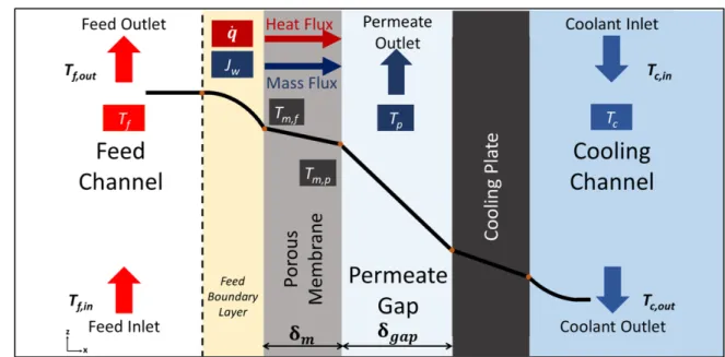
In the PGMD configuration (Fig. 1), a hydrophobic membrane is in direct contact with the feed 123
and permeate sides. It is assumed that the permeate gap is entirely filled with permeate liquid with 124
permeate overflow leaving the channel from the top. The permeate gap and coolant plate introduce 125
additional heat transfer resistances in the system (compared to DCMD), which have to be 126
considered in the PGMD model. The vapor flow through the membrane pores is induced by the 127
partial pressure difference between the feed and permeate sides. The total transmembrane mass 128
flux (J, kg/m2 s) can be defined as follows:
129
𝐽 = 𝐵7. 9𝑃7,<-.#− 𝑃7,#-.#> = 𝐵7 ∆𝑃-.# (1)
where Bm is the membrane distillation coefficient (kg/m2 Pa s), 𝑃7,<-.# is the vapor pressure on the
130
membrane/feed interface (Pa), 𝑃7,#-.# is the vapor pressure on the membrane/permeate gap interface 131
8
(Pa) and ∆𝑃-.# is the partial pressure difference between the feed and permeate gap sides. 𝑃 7,<-.#
132
and 𝑃7,#-.# depend on the temperatures at the membrane surface on the feed (𝑇7,<) and permeate
133
gap (𝑇7,#) sides, respectively. 134
135
136
Fig. 1. Schematic representation of PGMD configuration in the counter-current flow mode. The
137
configuration includes the feed channel with the feed boundary layer, the porous hydrophobic 138
membrane, the permeate gap channel, the cooling plate, and the cooling channel. Tf, Tp and Tc
139
represent the local bulk stream temperatures along the feed, permeate gap and cooling channels, 140
respectively. These temperatures vary along the channels due to the heat transfer along the module. 141
142
The vapor pressure of water (𝑃-.#) can be calculated by the Antoine equation [26]:
143
𝑃-.# = 𝑒𝑥𝑝 D23.1964 − 3816.44
𝑇 − 46.13L
(2)
where T is the temperature (K). Since pure water was used as the feed stream in our experiments, 144
vapor pressure depression was not considered in our model. 145
Mass and heat transfer occur simultaneously. The heat flux is a function of vapor flux, J. The 146
overall J can be calculated by integrating the local flux, J(y,z), over the full membrane surface as 147
follows: 148
9 𝐽 =1 𝐴N 𝐽(𝑦, 𝑧) 𝑑𝑦 𝑑𝑧 (3) 𝐽 =𝐵7 𝐴 N ∆𝑃-.#(𝑦, 𝑧) 𝑑𝑦 𝑑𝑧 (3a) 𝐽 =𝐵𝐴7TN 𝑃7,<-.#(𝑦, 𝑧) 𝑑𝑦 𝑑𝑧 − N 𝑃7,#-.#(𝑦, 𝑧) 𝑑𝑦 𝑑𝑧U (3b) where A is the active membrane area (m2) and the (y, z) coordinate represents the location on the
149
membrane surface at the feed/membrane or permeate gap/membrane interface. 150
The heat flux (𝑞̇) across the system components in the x-direction (Fig. 1) is the same under steady-151
state conditions 152
𝑞̇ = 𝑞̇VW,< = 𝑞̇7 = 𝑞̇#= 𝑞̇2 (4)
𝑞̇VW,< = ℎ< 9𝑇<− 𝑇7,<> (5)
where 𝑞̇VW,<, 𝑞̇7, 𝑞̇#, and 𝑞̇2 are the heat fluxes through the feed side boundary layer, the membrane, 153
the permeate gap and the cooling system, respectively. hf is the heat transfer coefficient for the
154
feed side boundary layer (W/m2 K). In this study, the heat transfer in the feed channel is evaluated
155
using the 3D CFD model. Based on this model, the heat transfer coefficient across the feed side 156
boundary layer can be inferred. 157
Membrane side 158
The overall heat flux through the membrane, 𝑞̇7, can be expressed as follows: 159
𝑞̇7 = 𝑞̇-.#+ 𝑞̇20,3 (6)
where 𝑞̇20,3 and 𝑞̇-.# are the conductive heat flux and the heat flux due to evaporation at the pore 160
entrance, respectively. Since the mass and heat transfer phenomena happen simultaneously, the 161
heat flux through the membrane thickness is a function of permeate flux, J, through the membrane. 162
Thus, 𝑞̇-.# can be expressed as
10
𝑞̇-.# = 𝐽 ℎ<Z (7)
where ℎ<Z is the latent heat of evaporation. Heat flux across the membrane thickness due to 164
conduction can be calculated from 165
𝑞̇20,3 =𝑘7
𝛿7 9𝑇7,<− 𝑇7,#> = ℎ7,20,3 ∆𝑇
(8)
where ∆𝑇 is the temperature difference between the opposing membrane sides, ℎ7,20,3 is the 166
membrane conductive heat transfer coefficient (W/m2 K) and 𝑘
7 is the thermal conductivity of
167
the membrane (W/m K), which is calculated from the simple approximation: 168
𝑘7 = 𝜀 𝑘Z.]+ (1 − 𝜀) 𝑘]01+3 (9)
where 𝑘Z.] is the thermal conductivity of the gas (air and vapor) trapped within the membrane
169
pores (W/m K), 𝑘]01+3 is the thermal conductivity of the solid membrane material (W/m K), and 𝜀 170
is the porosity of the membrane. The gas thermal conductivity is usually far lower than the solid 171
membrane conductivity, so in order to minimize the conductive heat losses 𝑘7 must be as low as 172
possible or 𝜀 high as high as possible. By substitution in Eqn. 6, 𝑞̇7 becomes: 173
𝑞̇7= 𝐽 ℎ<Z+ ℎ7,20,3. ∆𝑇 (10)
174
Permeate gap channel 175
In the permeate gap channel, permeate liquid fills the gap completely and the permeate overflow 176
leaves the channel from the top. Since the liquid in the channel is almost stagnant, heat transfer 177
through the permeate channel is by conduction only and there is no boundary layer on the 178
permeate-gap side of the membrane. The heat flux through the permeate gap, 𝑞̇#, can be expressed
179 as: 180
11
where hp is the heat transfer coefficient through the whole thickness of the permeate gap (W/m2
181
K) and 𝑇2,# is the temperature at the permeate gap/cooling plate interface. hp can also be expressed
182 as 183 ℎ# = 𝑘Z.# 𝛿Z.# (12)
where kgap and δgap are the thermal conductivity and thickness of the permeate gap, respectively.
184
If there is no spacer in the permeate gap channel, then 𝑞̇# is only determined by the thermal 185
conductivity of the fresh water (𝑘^./_`) in the gap (𝑘Z.# = 𝑘^./_`). Increasing 𝑘Z.# leads to better 186
process performance, the opposite effect of increasing 𝑘7 [7]. 187
Cooling system 188
Heat is transferred from the permeate gap to the coolant liquid via a combination of thermal 189
resistances including those of cooling plate and the cooling channel. 190 𝑞̇2 = ℎ2,/0/.1 9𝑇2,# − 𝑇2> (13) 1 ℎ2,/0/.1= 1 ℎ#1./_+ 1 ℎ2 (14) 191
where hc, total, ℎ#1./_ and ℎ2 represent the heat transfer coefficients through the cooling system, the
192
heat transfer coefficient through the cooling plate (hplate = kplate/δplate), and the heat transfer
193
coefficient through the cooling channel, respectively. 194
Thermal efficiency (η) is the fraction of energy transferred from the hot feed stream to the cold 195
permeate side that is actually utilized in mass transfer [17]. η is calculated from 196
𝜂 = 𝑄̇-.# 𝑄̇-.#+ 𝑄̇20,3
(15)
where 𝑄̇-.# is the rate of heat transfer from the feed to the permeate due to the mass transfer (W)
197
and 𝑄̇20,3 is the rate of heat transfer due to conduction through the membrane (𝑄̇20,3 = 𝑞̇20,3 𝐴). 198
12
When 𝜂 is close to unity, most of the heat delivered to the MD module is consumed via the 199
evaporation process and conductive heat losses are negligible. Membrane properties and MD 200
operational parameters have a significant influence on η [17]. 201
202
2.2 Governing transport equations in the CFD model
203
Since k-ε models have been validated and found reliable for various MD configurations (AGMD, 204
DCMD and VMD) [27–32], the realizable two-layer k- 𝜀 model was applied to model the turbulent 205
flow in the feed and permeate channels. A turbulent eddy-viscosity was considered as a function 206
of the turbulent kinetic energy (k) and turbulent dissipation rate (𝜀) terms in the model [33]. This 207
model is one of the Reynolds-Averaged Navier-Stokes equations which approximate the 208
representation of the physical phenomena of turbulence. The transport equations govern the 209
transport of the mean flow quantities. In order to model the stress tensor, the Reynolds stress 210
transport models and Boussinesq approximation (which is an eddy viscosity model) were 211
employed. Further details can be found in [34,35]. 212
The contributions of J and 𝑞̇-.# were included in the three Reynolds-averaged conservation
213
equations: conservation of mass (16), conservation of momentum (17) and conservation of energy 214 (18). 215 ∇. (𝜌𝑣⃗) = 𝑆g (16) ∇. (𝜌𝑣⃗𝑣⃗) = −∇P + ∇. (𝜏⃗)+𝜌𝑔⃗ + 𝑆7 (17) ∇. 9𝜌𝑐#𝑇𝑣⃗> = ∇. (𝑘∇𝑇)+𝑆j (18)
where Sj, Sm, and Sh are mass, momentum and energy source terms, respectively, and can be
216
calculated from [36] 217
𝑆g = k
−𝐽 𝐴𝑉 at the feed/membrane interface 𝐽 𝐴
𝑉 at the permeate gap/membrane interface
13 𝑆7 = k
−𝐽 𝐴 𝑢
𝑉 at the feed/membrane interface 𝐽 𝐴 𝑢
𝑉 at the permeate gap/membrane interface
(17a)
𝑆j = k − 𝑞̇-.#𝐴
𝑉 at the feed/membrane interface 𝑞̇-.#𝐴
𝑉 at the permeate gap/membrane interface
(18a)
where 𝑢 is the feed velocity (m/s) in the flow direction and V is the fluid element volume (m3).
218 219
3. Methodology
220 3.1. PGMD experimental set-up 221A laboratory scale PGMD setup was used for the experiments, as illustrated in Fig. 2. The 222
experimental setup has two flow loops for hot feed and coolant streams. Since MD in the counter-223
current flow mode (in terms of coolant and feed streams) has shown better performance than the 224
co-current mode [4], the experiments were performed in the former mode. The system included a 225
flat sheet hydrophobic PVDF membrane (ISEQ00010 Millipore). The module and membrane 226
properties are listed in Table 1. The membrane active area was 192 cm2. An aluminum plate was
227
used as the cooling plate. The feed and permeate channels had inner dimensions of 16 cm × 12 228
cm. A plastic spacer was used in the permeate gap channel to keep the permeate gap thickness 229
constant. Also, an additional woven spacer mesh was placed in between the membrane and plastic 230
spacer to protect the membrane from any damage due to the hard edges of the plastic mesh. In the 231
module, the design of the feed flow channel included a flow developing region before the feed 232
stream entrance to achieve a fully developed feed inlet flow condition when the feed stream 233
reached the active membrane area. Further details of the experimental apparatus are given in [37]. 234
14
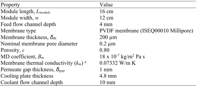
Table 1. PGMD module and membrane properties.
236
Property Value
Module length, Lmodule 16 cm
Module width, w 12 cm
Feed flow channel depth 4 mm
Membrane type PVDF membrane (ISEQ00010 Millipore)
Membrane thickness, δm 200 µm
Nominal membrane pore diameter 0.2 µm
Porosity, ε 0.80
MD coefficient, Bm 18 x 10-7 kg/m2 Pa s
Membrane thermal conductivity (km) a 0.07332 W/m K
Permeate gap thickness, δgap 1 mm
Cooling plate thickness 4.8 mm
Coolant flow channel depth 10 mm
a Calculated from Eq. (9) where 𝑘
Z.] is equal to the thermal conductivity of the vapor (𝑘-.#0`= 0.0261 W/m K) and 237
𝑘]01+3 is the thermal conductivity of the PVDF (𝑘nopq= 0.2622 W/m K) [38,39]. 238
239
3.2. PGMD Experimental procedure
240
The PGMD experiments were performed at four feed flow rates, 𝐹̇< (3.87, 7.94, 12.13, and 15.92 241
L/min). Pure water was used as feed solution in our experiments. The conductivity of the feed and 242
permeate water streams were measured to monitor for membrane wetting and purity of the 243
freshwater produced. The average feed conductivity was 298 µS/cm while the average permeate 244
conductivity remained below 11.8 µS/cm during the experiments. This guaranteed that pore 245
wetting was avoided during the experiments. The process operating conditions are summarized in 246
Table 2. First, the feed stream was heated to 63.4 °C at the adjusted pressure and 𝐹̇< condition. 247
Similarly, the cooling water was kept at 21.2 °C with a constant cooling water flow rate (𝐹̇2) of 248
10.99 L/min. The stream temperatures were monitored using pipe plug thermistor probes 249
(designated with temperature sensor symbol (T) in Fig. 2a). The 𝐹̇< values yielded a Reynolds 250
number range (2100 ≤ Re ≤ 9100), which includes the transition to turbulent flow regime. Stable 251
values were obtained for the flow rates and temperatures of the streams after 2.5 hours. Then, each 252
experiment was continued for an additional 1.5 hours to obtain a stable permeate flux (J) under 253
steady state condition. Each set of experiments was repeated three times to check repeatability. 254
Finally, the experimental data were compared with the CFD simulation results to validate the 255
developed model, which was also based on the same operating conditions used in the experiments. 256
15 257
258
Fig. 2. (a) Schematic representation of the PGMD experimental setup, (b) PGMD system parts: 1-
259
feed channel, 2- PVDF membrane, 3- permeate gap channel, 4- aluminum cooling plate, 5- coolant 260
channel and spacers (plastic and woven) along the permeate gap channel. 261
16
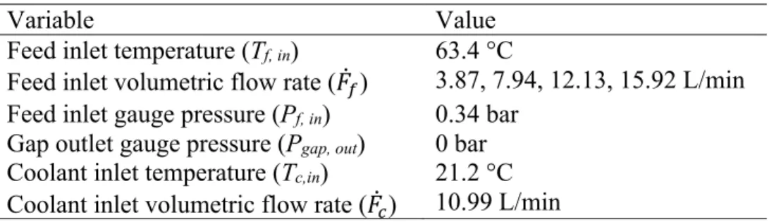
Table 2. Summary of the operating conditions during the PGMD experiments
263
Variable Value
Feed inlet temperature (Tf, in) 63.4 °C
Feed inlet volumetric flow rate (𝐹̇<) 3.87, 7.94, 12.13, 15.92 L/min Feed inlet gauge pressure (Pf, in) 0.34 bar
Gap outlet gauge pressure (Pgap, out) 0 bar
Coolant inlet temperature (Tc,in) 21.2 °C
Coolant inlet volumetric flow rate (𝐹̇2) 10.99 L/min
264
3.3. CFD model setup
265
The CFD model runs were performed using the CCM+ package (double precision Star-266
CCM+12.06.010-R8, Siemens Product Lifecycle Management Software Inc., Plano, Texas [33]). 267
In the CFD model, a steady-state condition was assumed within the PGMD process. Since the feed 268
and cooling channels flows were within the transition/turbulent flow ranges (2100 ≤ Re ≤ 9100 in 269
our experiments), a realizable two-layer k- 𝜀 turbulence model was applied. The feed, permeate 270
gap and coolant streams were set as freshwater. In the experiments, the permeate gap was filled 271
with stagnant permeate liquid. Additionally, a plastic spacer was placed in the channel to support 272
the membrane and keep the permeate gap thickness constant. Since the porosity of the spacer was 273
large (around 80%) and the thermal conductivity of water (kwater ≈ 0.60 W/m K) is much higher
274
than that of the plastic spacer (kspacer ≈ 0.15 W/m K), the thermal conductivity of the permeate gap
275
was considered to be that of freshwater in the baseline case in our CFD model (kwater ≈ 0.60 W/m
276
K). 277
Geometry and boundary conditions
278
The experimental conditions explained in the previous section and provided in Table 2, were used 279
as the basis of the CFD model. To develop the model, a three-dimensional geometry was built 280
based on the properties in Table 1. The general scheme of this geometry is presented in Fig. 3a. 281
The inset figure illustrates the module parts and the direction of the applied inlet and outlet 282
conditions on the boundaries. The feed, permeate gap, and cooling channels were set as fluid 283
domains and the membrane and cooling plate were defined as solid volumes. Feed inlet, feed 284
outlet, permeate outlet, coolant inlet, and coolant outlet boundaries were set based on the 285
experimental conditions given in Table 2. The boundaries for the inlets and outlets were set as 286
17
velocity inlets and pressure outlets, respectively. The coolant and permeate outlet boundaries were 287
open to atmospheric pressure. All the sidewall boundaries other than the inlet and outlet boundaries 288
were considered as no-slip walls. The internal interface boundaries (the feed/membrane interface, 289
the membrane/permeate gap interface, the permeate gap/cooling plate interface and the cooling 290
plate/cooling channel interface) were selected as conjugate heat transfer boundaries, which allow 291
conjugate heat transfer between the regions (between a fluid domain and a solid domain) in Star-292
CCM+. This strategy allows the simulation of heat transfer between a solid domain and a fluid 293
domain by exchanging thermal energy at the boundary between the two domains, so that heat 294
transport can be solved for at the wall correctly. In order to include the energy sink and source 295
terms, the heat flux was specified at the relevant interfaces such as the feed/membrane interface 296
(where energy leaves the feed volume), and the membrane/permeate gap interface (where energy 297
enters the permeate gap volume). Then, these terms were linked with an expression defined for 298
calculating 𝑞̇-.#. The mass and momentum source terms were similarly set and linked with an 299
expression defined for calculating J. J was monitored over a range of inlet feed volumetric flow 300
rates (𝐹̇<): 3.87, 7.94, 12.13, and 15.92 L/min. In the CFD model, the thermal conductivity of the
301
permeate gap (kgap = 0.6 W/m K) and membrane distillation coefficient (Bm = 18 x 10-7 kg/m2 s
302
Pa) were selected based on the reported data for a similar setup and the same type of membrane 303
[6]. 304
305
Fig. 3. (a) CAD drawing of the PGMD domain and its subdomain representation (Feed stream
306
entrance region and MD module subdomains including the feed, permeate gap and cooling 307
18
channels, and the PVDF membrane and cooling plate solid domains with the boundaries), (b) the 308
structure of the mesh from the top view of the PGMD module. 309
310
Mesh operation
311
The directed mesh operation was applied to generate a 3D solver mesh in Star-CCM+ [33]. A mesh 312
independence analysis was performed to achieve reliable results from the simulations. Permeate 313
flux was chosen as a comparison parameter to ensure that flux results are grid-size-independent. 314
The mesh size was refined step by step with considering all three dimensions and the permeate 315
flux results were compared. When the change in permeate flux was less than 1%, the mesh 316
refinement stopped. For the validation model, 240 number of divisions along the module length 317
and 120 number of divisions along the module width were created as a base for the directed mesh 318
operation. Then, the operation was continued for the feed channel, membrane, permeate gap, and 319
cooling channel thicknesses, which were divided into 40, 20 and 50 layers, respectively. A two-320
sided hyperbolic stretching factor was applied for the domains (spacing at the wall boundaries was 321
started at 0.01 mm.). The stretching factor was used to achieve further mesh refinement near the 322
wall boundaries and to monitor the boundary layers of the feed and cooling water streams. The 323
cooling plate and membrane were divided into 40 and 10 layers, respectively. Additionally, a 324
volume extruder was applied to create 20 cm entrance length before the feed inlet boundary. This 325
entrance region was included in the model to achieve a fully developed feed inlet condition when 326
the feed stream reaches the active membrane area. Heat losses were neglected at the entrance 327
region. In total, 1,305 x 104 elements were generated for the domain. The structure of the mesh
328
from the top view of the PGMD module is shown in Fig. 3b. 329
Software tool
330
A finite volume numerical discretization scheme based Star-CCM+ commercial software was used 331
to solve the model equations described above. Pre-processing step was also performed utilizing 332
the CAD and meshing packages provided in the Star-CCM+ software. SIMPLE algorithm was 333
implemented to control the overall solution. Segregated flow and segregated energy solvers were 334
set and the second-order upwind numerical scheme was used for the numerical solution. Under-335
relaxation factors (URFs) were defined for solvers such as velocity solver (URF= 0.7), pressure 336
solver (URF= 0.3), fluid energy (URF= 0.8), and solid energy (URF= 0.9). The URF value governs 337
19
the new level to which the newly computed data from the solution replaces the old data for each 338
iteration step [33]. J and 𝑞̇-.# were calculated and fed into the solution of the governing CFD 339
model equations (Eqs. 16‒ 18) through the source terms (Eqs. 16a‒18a) for each iteration step. It 340
continued until the solver converged to represent the local hydrodynamic and thermal properties 341
within the solution domain. The convergence criteria were achieved when the flow rate of fluid 342
entering and leaving the model balanced and the temperature and J plots became stable. The 343
residuals of the continuity and momentum equations were maintained below 10-12, and the residual
344
of the energy equation was maintained below 10-5. It took an average 45,000 iterations to reach
345
the residual levels. 346
347
3.4. Design of the simulation runs: Two-level full factorial design
348
Factorial analysis is a useful statistical approach, which can be applied in the design of both 349
experiments and modeling studies [40]. The technique is used to study the impact of multiple 350
independent variables, each of which may assume different possible values (i.e., levels), on one or 351
more dependent variables. All potential high and low combinations of the input factors were 352
considered in a two-level full factorial design to plan the runs for an experimental or modeling 353
study [24,25,40]. Design-Expert ® Version 10 (Stat-Ease Inc., Minneapolis [41]) was used to 354
design the simulation runs. The relative effects of four selected key factors and their interactions 355
were elucidated in this study: kgap, δgap, Lmodule and Bm. A CFD simulation was performed for each
356
run under the process operating conditions provided earlier (Table 2). 357
The following inputs were used in all simulation runs; Tf, in = 63.4 °C, 𝐹̇< =3.87 L/min, Pgap,out = 0
358
bar (gauge pressure), Tc,in = 21.2 °C, and 𝐹̇2 = 10.99 L/min. The module and membrane properties
359
were the same as in Table 1, but the selected four variables (kgap, δgap, Lmodule, and Bm) were varied
360
for each run. The design matrix of the runs at two levels of input parameters (lower‒ and upper‒ 361
bounded intervals) are presented in Table 3. The positive (+) and negative (‒) signs for each factor 362
indicate two-levels which are the lower and upper bounds, respectively. The total number of factor 363
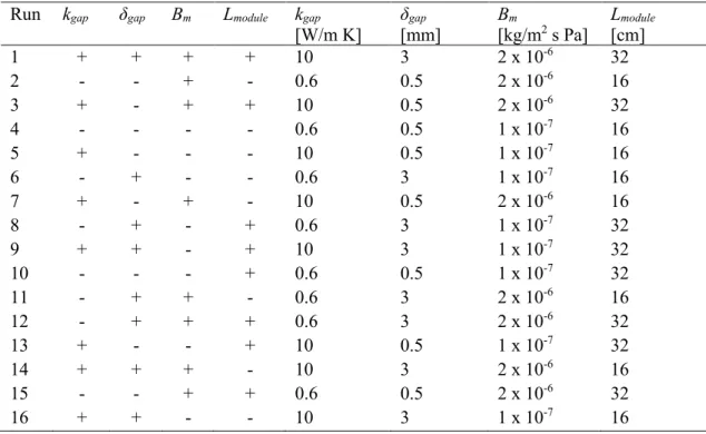
combinations is based on the 2, rule [25], where n is the number of factors (4 in this case).
364
The levels (lower and upper bounds) were selected based on a thorough review of the reported 365
values for each factor found in the literature. For instance, since increasing kgap or Bm does not
20
have a significant influence on the permeate flux beyond a specific limit [4,6], the upper bounds 367
of the kgap and Bm were set at 10 W/m K and 20 x 10-7 kg/m2 s Pa, respectively. The lower bound
368
of the kgap was kept equal to the thermal conductivity of water, which is 0.6 W/m K. The responses
369
(J and η) from each CFD run were fed into the Design-Expert software to analyze the effects of 370
factors statistically. A 95% confidence level was used in the analysis. 371
372
Table 3. Design matrix table for the CFD simulation runs based on a two-level full factorial design
373
(four main factors: gap conductivity (kgap), gap thickness (δgap), MD coefficient (Bm) and module
374
length (Lmodule)). A total of 16 CFD runs were performed.
375
Run kgap δgap Bm Lmodule kgap
[W/m K] δgap [mm] Bm [kg/m2 s Pa] L[cm] module 1 + + + + 10 3 2 x 10⁻⁶ 32 2 - - + - 0.6 0.5 2 x 10⁻⁶ 16 3 + - + + 10 0.5 2 x 10⁻⁶ 32 4 - - - - 0.6 0.5 1 x 10⁻⁷ 16 5 + - - - 10 0.5 1 x 10⁻⁷ 16 6 - + - - 0.6 3 1 x 10⁻⁷ 16 7 + - + - 10 0.5 2 x 10⁻⁶ 16 8 - + - + 0.6 3 1 x 10⁻⁷ 32 9 + + - + 10 3 1 x 10⁻⁷ 32 10 - - - + 0.6 0.5 1 x 10⁻⁷ 32 11 - + + - 0.6 3 2 x 10⁻⁶ 16 12 - + + + 0.6 3 2 x 10⁻⁶ 32 13 + - - + 10 0.5 1 x 10⁻⁷ 32 14 + + + - 10 3 2 x 10⁻⁶ 16 15 - - + + 0.6 0.5 2 x 10⁻⁶ 32 16 + + - - 10 3 1 x 10⁻⁷ 16 376
4. Results and Discussion
377
4.1. CFD model validation
378
The developed CFD model was validated using the experimentally obtained data over a range of 379
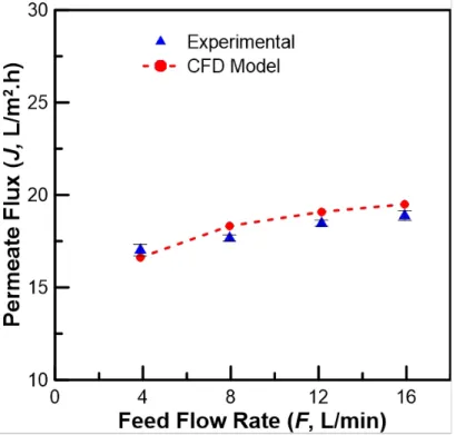
feed inlet volumetric flow rates, 𝐹̇< = 3.87, 7.94, 12.13, and 15.92 L/min. The permeate flux, J, 380
predictions from the CFD model were plotted against 𝐹̇< in Fig. 4, along with their corresponding 381
experimental values. Since the CFD model results are very close to the experimental data, the CFD 382
predictions were deemed in good agreement with the experimental results. As shown in Fig. 4., 383
21
higher feed flow rates result in enhanced water flux, due to the increase in the local heat transfer 384
coefficient at the feed side (hf). The thermal boundary layer at the feed side becomes thinner with
385
increasing 𝐹̇< and the temperature polarization effect diminishes [10,14,20]. 386
387
388 389
Fig. 4. CFD model validation using experimental permeate flux measurements over a range of
390
feed flow rates (𝐹̇< = 3.87, 7.94, 12.13 and 15.92 L/min).
391 392
The mentioned effect of feed flow rate on hf was further examined using the CFD results. hf was
393
monitored along the membrane length at the membrane/feed interface for four 𝐹̇< values, as 394
presented in Fig. 5a. The shown hf values were calculated at the centerline of the feed-side
395
boundary layer (Fig. 5b). Using a feed flow rate of 3.87 L/min as an example, the contour plot in 396
Fig. 5b shows the hf profile at the membrane/feed interface. Additionally, the thermal boundary
397
layer on the feed side was monitored and contour plots were generated at the feed/membrane 398
interface for the four feed flow rates (Fig. 6). The boundary layer thickness was monitored using 399
the “wall distance” field function in Star-CCM+. The thermal boundary layer, shown in terms of 400
distance from the membrane surface in Fig. 6, was defined as any location where the temperature 401
22
is less than 99% of the bulk stream temperature. The contour plots in Fig. 6 clearly show that as 402
𝐹̇< increased, the thermal boundary layers became thinner, which supports the reasoning behind 403
the results in Fig. 5. 404
405
406
Fig. 5. (a) Local heat transfer coefficient (h) along the module length (Lmodule) at the centerline of
407
the feed channel boundary layer for varying feed inlet volumetric flow rates (𝐹̇<= 3.87, 7.94, 408
12.13 and 15.92 L/min). (b) Contour plot which shows the distribution of h along the feed side 409
boundary layer near the membrane/feed interface (𝐹̇< = 3.87 L/min).
410 411
23 412
Fig. 6. Wall distance contour plots showing the change in thermal boundary layer thickness upon
413
varying the feed flow rates: (a) 𝐹̇< = 3.87 L/min (b) 𝐹̇< = 7.94 L/min (c) 𝐹̇< = 12.13 L/min and (d)
414
𝐹̇< = 15.92 L/min. 415
24
4.2. Effects of system factors on J and η
416
After its validation, the CFD model was used to investigate the effects of the four system factors 417
on J and η, based on the two-level full factorial design (table 3). The J and η values obtained from 418
the CFD simulations are listed in Table 4. Different trends can be observed from the simulation 419
results, which are in agreement with the literature-reported trade-offs between J and η for different 420
MD configurations [42,43]. Run 7 yielded the highest J value, while the highest value for η was 421
observed in Runs 11 and 12. Increasing Lmodule resulted in only a slight reduction of flux, which
422
can be expected given the fact that even the longest module modeled (32 cm) is still relatively 423
short (in comparison to full-scale MD systems), with tangible impacts of Lmodule hard to observe.
424
Similarly, increasing Lmodule did not influence η, for the same reason as J. It merits mentioning that
425
at significantly longer modules, both J and η are very likely to be affected in various ways, as we 426
demonstrated in a previous study for DCMD and AGMD systems [40]. However, as a result of the 427
fine grid used in our CFD modeling, which was needed to capture boundary layer effects, modeling 428
much longer modules (e.g., on the order of meters) would have required a massive computational 429
power unavailable to us. 430
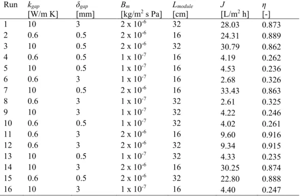
Table 4. Design matrix table for responses (J and η) from the CFD model simulations at the two
431
levels of four input factors (kgap, δgap, Bm, and Lmodule). 𝐹̇< was assumed 3.87 L/min (constant)
432 Run kgap [W/m K] δgap [mm] Bm [kg/m2 s Pa] L[cm] module J [L/m2 h] η [-] 1 10 3 2 x 10⁻⁶ 32 28.03 0.873 2 0.6 0.5 2 x 10⁻⁶ 16 24.31 0.889 3 10 0.5 2 x 10⁻⁶ 32 30.79 0.862 4 0.6 0.5 1 x 10⁻⁷ 16 4.19 0.262 5 10 0.5 1 x 10⁻⁷ 16 4.53 0.236 6 0.6 3 1 x 10⁻⁷ 16 2.68 0.326 7 10 0.5 2 x 10⁻⁶ 16 33.43 0.863 8 0.6 3 1 x 10⁻⁷ 32 2.61 0.325 9 10 3 1 x 10⁻⁷ 32 4.22 0.246 10 0.6 0.5 1 x 10⁻⁷ 32 4.02 0.261 11 0.6 3 2 x 10⁻⁶ 16 9.60 0.916 12 0.6 3 2 x 10⁻⁶ 32 9.34 0.915 13 10 0.5 1 x 10⁻⁷ 32 4.33 0.235 14 10 3 2 x 10⁻⁶ 16 30.25 0.874 15 0.6 0.5 2 x 10⁻⁶ 32 22.80 0.888 16 10 3 1 x 10⁻⁷ 16 4.40 0.247 433
25
Effects of factors on flux
434
The Pareto chart in Fig. 7 represents the significance level of the individual and interconnected 435
factors on J in the dimensionless statistical form. The dimensionless statistical form aligns the 436
ranking based on the standard deviations at a set confidence level (95% was used in our analysis). 437
The t-value limit shown was calculated based on the identified significant parameters using half-438
normal plot, a tool which utilizes the ordered estimated effects in order to find the important factors 439
under the 95% of significance threshold condition, using the Design-Expert software [25,41,44]. 440
The blue columns indicate factors that are inversely proportional to the process output (J), while 441
the orange columns indicate a direct proportionality. The factors/factor interactions are ranked 442
from 1 to 15 based on the significance level. The bars below the t-value limit (rank 8 to rank 15) 443
represent factors/ interactions which do not have any significant effects on J. 444
445
446
Fig. 7. Pareto chart of the effects of factors/factor interactions on J where the t-value of the absolute
447
effects is plotted against the ranking. Rank 1 has the highest significance and 7 has the lowest 448
significance. The bars below the t-value limit represent factors/ interactions which do not have any 449
significant effects on J. The blue columns indicate factors that are inversely proportional to the 450
process output (J), while the orange columns indicate a direct proportionality. 451
26 452
Based on the results shown in Fig. 7, J was found directly proportional to Bm,as expected from Eq.
453
1, with Bm having the most significant effect on J. Since a high gap conductance (kgap/δgap) is
454
necessary for better process performance [6,7], kgap and δgap were the following factors in terms of
455
impact, although the interaction of kgap ‒ Bm was more important than δgap. The influence of Lmodule
456
was not as significant as those of other factors and interactions, as mentioned earlier. 457
Two types of interaction plots are given in Fig. 8 to further understand the above-mentioned trends. 458
In the 3D contour plots in Fig. 8, the x-axis and z-axis (horizontal axes) present the two factors of 459
interest, while the y-axis (vertical axis) shows the J values from the CFD model runs. The 460
remaining two factors (other than the two on the horizontal axes) were maintained at average 461
values when plotting the graphs. In the 2D interaction plots, J was plotted against one factor on 462
the x-axis. The two lines in each 2D interaction plot represent the upper- and lower-bounds of one 463
additional factor (the second factor of interest). Similar to the 3D contour plots, the remaining two 464
factors (other than those shown in the 2D interaction graph), were maintained at average values. 465
Interesting observations can be made from the graphs. The A‒C plots illustrate the interaction 466
between kgap and Bm. Even though the effect of kgap on flux was significant for membranes with
467
high Bm (20 x 10-7 kg/m2 Pa s), it had almost no effect on flux for the membrane with low Bm (1 x
468
10-7 kg/m2 Pa s). A similar observation can be made for δ
gap from the B‒C plots. δgap was inversely
469
proportional to J at high Bm (20 x 10-7 kg/m2 Pa s) and an increase in δgap from 0.5 mm to 3 mm
470
enhanced the flux as expected [8]. But, at low Bm (1 x 10⁻⁷ kg/m2 Pa s), this effect was very minute.
471
On the other hand, the kgap ‒ δgap interaction (on the A‒B plots) showed that the effect of kgap on J
472
was more evident at the higher δgap value (3 mm).
473
The flux is driven by the overall temperature difference between the hot and cold streams. The 474
resistance of the hot stream, membrane, gap, condensation plate and the cold stream are in series. 475
Since these resistances are in series, the total resistance between the hot and cold channels can be 476
evaluated as the sum of all the resistances (extending Eq. 14 across all the resistance terms). Within 477
the membrane, the resistances to vapor transport and to conduction can be considered to be in 478
parallel, since they represent two alternative pathways for heat transfer through the membrane. 479
If one of these 5 resistances is significantly larger than the rest, the sum is dominated by this 480
resistance. In such a scenario, changing this resistance would have a significant impact on overall 481
27
heat transfer, whereas modifying the others would have minimal impact. In light of this discussion, 482
we can understand the trends observed in Fig. 8. At low Bm, the membrane is the major resistance
483
in the series. In this scenario, therefore, changing kgap has a small influence on flux. In contrast, at
484
high Bm, the gap itself is the major resistance. Therefore, increasing kgap in this case leads to
485
significant improvement in flux. The observed trends of the impact of δgap at the different values
486
of Bm can also be explained by the same logic.
487
Similarly, at large δgap, the gap resistance is larger. In such a scenario, changes to the gap resistance
488
by changing kgap are more significant, rather than when δgap is small and the gap resistance itself
489
is correspondingly small. 490
491
492
Fig. 8. 3D contour and 2D interaction graphs for the permeate flux (J) response, where A‒C is the
493
kgap ‒ Bm interaction, B‒C is the δgap ‒ Bm interaction, and A‒B is the kgap ‒ δgap interaction. The
494
error bars in the 2D graphs indicate the 95% least significant difference interval for the data points. 495
28
Effects of factors on thermal efficiency
497
The Pareto chart in Fig. 9 displays the impact ranking of the different factors/factor interactions 498
on η based on the CFD simulations results in Table 4. The blue columns indicate factors that are 499
inversely proportional to the process output (η), while the orange columns indicate direct 500
proportionality. The factors/factor interactions are ranked from 1 to 15 based on the significance 501
level. The bars below the t-value limit (rank 1 to rank 4) indicate factors/interactions without any 502
significant effects on η. The results show that Bm, kgap, and δgap all have effects on η, with Bm
503
having, by far, the most significant effect. The significance levels of kgap and δgap followed, in that
504
order. The only significant factor interaction vis-à-vis η was the kgap ‒ δgap interaction, which came
505
fourth in the rank of significance. This factor interaction is presented in the 2D interaction and 3D 506
contour graphs in Fig. 9. Based on the heat transfer mechanism in PGMD, an increase in gap 507
conductance (kgap/δgap) is necessary to achieve better process performance [6,7]. Therefore, the
508
significance of the kgap ‒ δgap interaction was observed as expected.
509
Going back to the heat transfer resistance model of the MD process, η defines the fraction of the 510
total energy transfer happening in the form of vapor flux through the membrane. Not surprisingly 511
therefore, the permeability has a significant impact on η. An increase in Bm improves vapor
512
transport through the membrane without affecting the heat conduction resistance, thereby 513
significantly improving η. 514
29 515
Fig. 9. Pareto chart of the effects of factors/factor interactions on η where the t-value of the
516
absolute effects is plotted against the ranking. Rank 1 has the highest significance and 4 has the 517
lowest significance. The bars below the t-value limit represent factors/interactions which do not 518
have any significant effects on η. The blue columns indicate factors that are inversely proportional 519
to the process output (η), while the orange columns indicate direct proportionality. 520
521
522
Fig. 10. 3D contour and 2D interaction graphs for the η process output obtained from CFD model
523
runs. A‒B is the kgap ‒ δgap interaction.
30
5. Conclusion
525
In this study, a CFD model was developed for the PGMD configuration and was validated using 526
experimental data. Upon validation of the model, a factorial analysis statistical tool was used to 527
design the simulation sets to evaluate the influence of four selected PGMD configuration 528
parameters (kgap, δgap, Lmodule and Bm) on flux, J, and thermal efficiency, η. The latter two were
529
selected as key indicators of process performance. The model reveals the influence of module 530
design parameters in maximizing both J and η. The results show that Bm, kgap, and δgap each have
531
a significant contribution to PGMD process performance. Additionally, factorial analysis was a 532
useful tool to probe the significance of each factor by also considering the interactions among 533
parameters. 534
In view of the analysis, the following conclusions were reached: 535
• The membrane distillation coefficient has the most substantial effect on J and η in PGMD. 536
This term has a positive correlation with both J and η. 537
• The next largest effects are from kgap (positive correlation with J) and δgap (negative
538
correlation with J), individually, although the effect the kgap ‒ Bm interaction is more
539
significant than δgap with respect to its impact on J.
540
• The kgap ‒ Bm (positive correlation with J), δgap ‒ Bm (negative correlation with J), and kgap
541
‒ δgap (positive correlation with J) interactions all have significant impacts on J, in the order
542
listed. 543
• The effect of kgap on J is more significant for membranes with high Bm, because the gap
544
resistance becomes the dominant resistance at high Bm.
545
• The only significant factor interaction observed for η was that of kgap ‒ δgap. This interaction
546
has a negative correlation with η. 547
548
Acknowledgment
549
This work was supported by Khalifa University funding through the Center for Membrane and 550
Advanced Water Technology. The first author is also grateful for the support she received from 551
Massachusetts Institute of Technology during her research visit there, where the experimental part 552
of this work was conducted. 553
31
References
554
[1] N. Thomas, M.O. Mavukkandy, S. Loutatidou, H.A. Arafat, Membrane distillation research 555
& implementation: Lessons from the past five decades, Sep. Purif. Technol. 189 (2017) 556
108–127. doi:10.1016/j.seppur.2017.07.069. 557
[2] L. Eykens, I. Hitsov, K. De Sitter, C. Dotremont, L. Pinoy, I. Nopens, B. Van der Bruggen, 558
Influence of membrane thickness and process conditions on direct contact membrane 559
distillation at different salinities, J. Memb. Sci. 498 (2016) 353–364. 560
doi:10.1016/j.memsci.2015.07.037. 561
[3] E. Drioli, A. Ali, F. Macedonio, Membrane distillation: Recent developments and 562
perspectives, Desalination. 356 (2015) 56–84. doi:10.1016/j.desal.2014.10.028. 563
[4] J. Swaminathan, H.W. Chung, D.M. Warsinger, F.A. AlMarzooqi, H.A. Arafat, J.H. 564
Lienhard, Energy efficiency of permeate gap and novel conductive gap membrane 565
distillation, J. Memb. Sci. 502 (2016) 171–178. doi:10.1016/j.memsci.2015.12.017. 566
[5] L. Cheng, Y. Zhao, P. Li, W. Li, F. Wang, Comparative study of air gap and permeate gap 567
membrane distillation using internal heat recovery hollow fiber membrane module, 568
Desalination. 426 (2018) 42–49. doi:10.1016/j.desal.2017.10.039. 569
[6] J. Swaminathan, H.W. Chung, D.M. Warsinger, J.H. Lienhard V, Membrane distillation 570
model based on heat exchanger theory and configuration comparison, Appl. Energy. 184 571
(2016) 491–505. doi:10.1016/j.apenergy.2016.09.090. 572
[7] J. Swaminathan, H.W. Chung, D.M. Warsinger, J.H. Lienhard V, Energy efficiency of 573
membrane distillation up to high salinity: Evaluating critical system size and optimal 574
membrane thickness, Appl. Energy. 211 (2018) 715–734. 575
doi:10.1016/j.apenergy.2017.11.043. 576
[8] L. Eykens, T. Reyns, K. De Sitter, C. Dotremont, L. Pinoy, B. Van der Bruggen, How to 577
select a membrane distillation configuration? Process conditions and membrane influence 578
unraveled, Desalination. 399 (2016) 105–115. doi:10.1016/j.desal.2016.08.019. 579
[9] R.G. Raluy, R. Schwantes, V.J. Subiela, B. Peñate, G. Melián, J.R. Betancort, Operational 580
experience of a solar membrane distillation demonstration plant in Pozo Izquierdo-Gran 581
32
Canaria Island (Spain), Desalination. 290 (2012) 1–13. doi:10.1016/j.desal.2012.01.003. 582
[10] L. Francis, N. Ghaffour, A.A. Alsaadi, G.L. Amy, Material gap membrane distillation: A 583
new design for water vapor flux enhancement, J. Memb. Sci. 448 (2013) 240–247. 584
doi:10.1016/j.memsci.2013.08.013. 585
[11] J. Swaminathan, Unified Framework to Design Efficient Membrane Distillation for Brine 586
Concentration, (2017) 1–219. 587
[12] H. Cho, Y.-J. Choi, S. Lee, J. Koo, T. Huang, Comparison of hollow fiber membranes in 588
direct contact and air gap membrane distillation (MD), Desalin. Water Treat. (2015) 1–8. 589
doi:10.1080/19443994.2015.1038113. 590
[13] D. Winter, J. Koschikowski, M. Wieghaus, Desalination using membrane distillation: 591
Experimental studies on full scale spiral wound modules, J. Memb. Sci. 375 (2011) 104– 592
112. doi:10.1016/j.memsci.2011.03.030. 593
[14] A. Cipollina, M.G. Di Sparti, A. Tamburini, G. Micale, Development of a Membrane 594
Distillation module for solar energy seawater desalination, Chem. Eng. Res. Des. 90 (2012) 595
2101–2121. doi:10.1016/j.cherd.2012.05.021. 596
[15] D. Winter, Membrane distillation – a thermodynamic, technological and economic analysis 597
Ph.D. thesis, 2014. 598
[16] A. Deshmukh, C. Boo, V. Karanikola, S. Lin, A.P. Straub, T. Tong, D.M. Warsinger, M. 599
Elimelech, Membrane distillation at the water-energy nexus: Limits, opportunities, and 600
challenges, Energy Environ. Sci. 11 (2018) 1177–1196. doi:10.1039/c8ee00291f. 601
[17] A. Deshmukh, M. Elimelech, Understanding the impact of membrane properties and 602
transport phenomena on the energetic performance of membrane distillation desalination, 603
J. Memb. Sci. 539 (2017) 458–474. doi:10.1016/j.memsci.2017.05.017. 604
[18] F. Mahmoudi, G. Moazami Goodarzi, S. Dehghani, A. Akbarzadeh, Experimental and 605
theoretical study of a lab scale permeate gap membrane distillation setup for desalination, 606
Desalination. 419 (2017) 197–210. doi:10.1016/j.desal.2017.06.013. 607
[19] A. Hagedorn, G. Fieg, D. Winter, J. Koschikowski, T. Mann, Methodical design and 608
operation of membrane distillation plants for desalination, Chem. Eng. Res. Des. 125 (2017) 609
33 265–281. doi:10.1016/j.cherd.2017.07.024. 610
[20] A. Ruiz-Aguirre, J.A. Andrés-Mañas, J.M. Fernández-Sevilla, G. Zaragoza, Modeling and 611
optimization of a commercial permeate gap spiral wound membrane distillation module for 612
seawater desalination, Desalination. 419 (2017) 160–168. doi:10.1016/j.desal.2017.06.019. 613
[21] H. Ahadi, J. Karimi-Sabet, M. Shariaty-Niassar, T. Matsuura, Experimental and numerical 614
evaluation of membrane distillation module for oxygen-18 separation, (2018). 615
doi:10.1016/j.cherd.2018.01.042. 616
[22] I. Hitsov, T. Maere, K. De Sitter, C. Dotremont, I. Nopens, Modelling approaches in 617
membrane distillation: A critical review, Sep. Purif. Technol. 142 (2015) 48–64. 618
doi:10.1016/j.seppur.2014.12.026. 619
[23] M.M.A. Shirazi, A. Kargari, A.F. Ismail, T. Matsuura, Computational Fluid Dynamic 620
(CFD) opportunities applied to the membrane distillation process: State-of-the-art and 621
perspectives, Desalination. 377 (2016) 73–90. doi:10.1016/j.desal.2015.09.010. 622
[24] R.W. Mee, A Comprehensive Guide to Factorial Two-Level Experimentation, Springer, 623
2009. 624
[25] J. Antony, Design of Experiments for Engineers and Scientists, Second edi, Elsevier, 2014. 625
doi:10.1016/B978-0-08-099417-8. 626
[26] M. Essalhi, M. Khayet, Fundamentals of membrane distillation, Elsevier Ltd, 2015. 627
doi:10.1016/B978-1-78242-246-4.00010-6. 628
[27] E. Karbasi, J. Karimi-Sabet, J. Mohammadi-Rovshandeh, M. Ali Moosavian, H. Ahadi, Y. 629
Amini, Experimental and numerical study of air-gap membrane distillation (AGMD): Novel 630
AGMD module for Oxygen-18 stable isotope enrichment, Chem. Eng. J. 322 (2017) 667– 631
678. doi:10.1016/j.cej.2017.03.031. 632
[28] A.N. Mabrouk, , Yasser Elhenawy, M. Abdelkader, M. Shatat, The impact of baffle 633
orientation on the performance of the hollow fiber membrane, Desalin. Water Treat. 58 634
(2017) 35–45. doi:10.5004/dwt.2017.0030. 635
[29] L. Zhang, J. Xiang, P.G. Cheng, N. Tang, H. Han, L. Yuan, H. Zhang, S. Wang, X. Wang, 636
Three-dimensional numerical simulation of aqueous NaCl solution in vacuum membrane 637
34
distillation process, Chem. Eng. Process. Process Intensif. 87 (2015) 9–15. 638
doi:10.1016/j.cep.2014.11.002. 639
[30] X. Yang, H. Yu, R. Wang, A.G. Fane, Analysis of the effect of turbulence promoters in 640
hollow fiber membrane distillation modules by computational fluid dynamic (CFD) 641
simulations, J. Memb. Sci. 415–416 (2012) 758–769. doi:10.1016/j.memsci.2012.05.067. 642
[31] X. Yang, H. Yu, R. Wang, A.G. Fane, Optimization of microstructured hollow fiber design 643
for membrane distillation applications using CFD modeling, J. Memb. Sci. 421–422 (2012) 644
258–270. doi:10.1016/j.memsci.2012.07.022. 645
[32] N. Tang, H. Zhang, W. Wang, Computational fluid dynamics numerical simulation of 646
vacuum membrane distillation for aqueous NaCl solution, Desalination. 274 (2011) 120– 647
129. doi:10.1016/j.desal.2011.01.078. 648
[33] Siemens Product Lifecycle Management Software Inc, Star-CCM+, (2018). 649
[34] V.Y. Agbodemegbe, X. Cheng, E.H.K. Akaho, F.K.A. Allotey, Correlation for cross-flow 650
resistance coefficient using STAR-CCM+ simulation data for flow of water through rod 651
bundle supported by spacer grid with split-type mixing vane, Nucl. Eng. Des. 285 (2015) 652
134–149. doi:10.1016/j.nucengdes.2015.01.003. 653
[35] V.Y. Agbodemegbe, X. Cheng, E.H.K. Akaho, F.K.A. Allotey, An investigation of the 654
effect of split-type mixing vane on extent of crossflow between subchannels through the 655
fuel rod gaps, Ann. Nucl. Energy. 88 (2016) 174–185. doi:10.1016/j.anucene.2015.10.036. 656
[36] B. Lian, Y. Wang, P. Le-Clech, V. Chen, G. Leslie, A numerical approach to module design 657
for crossflow vacuum membrane distillation systems, J. Memb. Sci. 510 (2016) 489–496. 658
doi:10.1016/j.memsci.2016.03.041. 659
[37] J.B. Swaminathan, Numerical and Experimental Investigation of Membrane Distillation 660
Flux and Energy Efficiency, (2014). 661
[38] C.Y. Iguchi, W.N. dos Santos, R. Gregorio, Determination of thermal properties of 662
pyroelectric polymers, copolymers and blends by the laser flash technique, Polym. Test. 26 663
(2007) 788–792. doi:10.1016/j.polymertesting.2007.04.009. 664
[39] H. Yu, X. Yang, R. Wang, A.G. Fane, Numerical simulation of heat and mass transfer in 665
35
direct membrane distillation in a hollow fiber module with laminar flow, J. Memb. Sci. 384 666
(2011) 107–116. doi:10.1016/j.memsci.2011.09.011. 667
[40] M.I. Ali, E.K. Summers, H.A. Arafat, J.H. Lienhard V, Effects of membrane properties on 668
water production cost in small scale membrane distillation systems, Desalination. 306 669
(2012) 60–71. doi:10.1016/j.desal.2012.07.043. 670
[41] Stat-Ease Inc., Design-Expert® Version 10, (2018). 671
[42] X. Yang, R. Wang, A.G. Fane, Novel designs for improving the performance of hollow 672
fiber membrane distillation modules, J. Memb. Sci. 384 (2011) 52–62. 673
doi:10.1016/j.memsci.2011.09.007. 674
[43] Q. He, P. Li, H. Geng, C. Zhang, J. Wang, H. Chang, Modeling and optimization of air gap 675
membrane distillation system for desalination, Desalination. 354 (2014) 68–75. 676
doi:10.1016/j.desal.2014.09.022. 677
[44] M. Shah, K. Pathak, Development and Statistical Optimization of Solid Lipid Nanoparticles 678
of Simvastatin by Using 23 Full-Factorial Design, AAPS PharmSciTech. 11 (2010) 489– 679
496. doi:10.1208/s12249-010-9414-z. 680