A Comparison of Data Association Techniques for
Simultaneous Localization and Mapping
by Aron J. Cooper
B.A.E.M Aerospace Engineering and Mechanics, University of Minnesota, 2003 B.S. Astrophysics, University of Minnesota, 2003
SUBMITTED TO THE DEPARTMENT OF AERONAUTICS AND ASTRONAUTICS IN PARTIAL FULFILLMENT OF THE REQUIREMENTS FOR THE DEGREE OF
MASTER OF SCIENCE IN AERONAUTICS AND ASTRONAUTICS AT THE
MASSACHUSETTS INSTITUTE OF TECHNOLOGY JUNE 2005
@ Aron J. Cooper, 2005. All rights reserved.
The author hereby grants to MIT permission to reproduce and distribute publicly paper and electronic copies of this thesis document in whole or in part.
Author:
rtment of Aeronautics and Astronautics May 20, 2005 Certified
by:-Nicholas Roy, Ph.D. Assistant Professor of Aeronautics and Astronautics Thesis Supervisor Certified by:
Don Gustafson, Ph.D. Distinguished Member of the Technical Staff, C. S. Draper Laboratory Thesis Supervisor Certified by-
Marc McConley, Ph.D. Principal Memer of the Technical Staff, C. S. Draper Laboratory Thesis Supervisor Accepted
by:-James Peraire, Ph.D. Professor of Aeronautics and Astronautics Chair, Committee on Graduate Students
OF TECHNOLOGY
N.
N.
A Comparison of Data Association Techniques for Simultaneous
Localization and Mapping
by
Aron J. Cooper
Submitted to the Department of Aeronautics and Astronautics on May 20, 2005, in partial fulfillment of the
requirements for the degree of
Master of Science in Aeronautics and Astronautics
Abstract
The problem of Simultaneous Localization and Mapping (SLAM) has received a great deal of attention within the robotics literature, and the importance of the solutions to this problem has been well documented for successful operation of autonomous agents in a number of environments. Of the numerous solutions that have been developed for solving the SLAM problem many of the most successful approaches continue to either rely on, or stem from, the Extended Kalman Filter method (EKF). However, the new algorithm FastSLAM has attracted attention for many properties not found in EKF based methods. One such property is the ability to deal with unknown data association and its robustness to data association errors.
The problem of data association has also received a great deal of attention in the robotics literature in recent years, and various solutions have been proposed. In an effort to both compare the performance of the EKF and FastSLAM under ambiguous data asso-ciation situations, as well as compare the performance of three different data assoasso-ciation methods a comprehensive study of various SLAM filter-data association combinations is performed. This study will consist of pairing the EKF and FastSLAM filtering ap-proaches with the Joint Compatibility, Sequential Compatibility Nearest Neighbor, and Joint Maximum Likelihood data association methods. The comparison will be based on both contrived simulations as well as application to the publicly available Car Park data
set.
The simulated results will demonstrate a heavy dependence on geometry, particularly landmark separation, for the performance of both filter performance and the data associ-ation algorithms used. The real world data set results will demonstrate that the perfor-mance of some data association algorithms, when paired with an EKF, can give identical results. At the same time a distinction in mapping performance between those pairings and the EKF paired with Joint Compatibility data association will be shown. These EKF based pairings will be contrasted to the performance obtained for the FastSLAM-Sequential Nearest Neighbor marriage. Finally, the difficulties in applying the Joint Com-patibility and Joint Maximum Likelihood data association methods using FastSLAM 1.0 for this data set will be discussed.
Thesis Supervisor: Nicholas Roy, Ph.D.
Title: Assistant Professor of Aeronautics and Astronautics Thesis Supervisor: Don Gustafson, Ph.D.
Title: Distinguished Member of the Technical Staff, C. S. Draper Laboratory Thesis Supervisor: Marc McConley, Ph.D.
Acknowledgments
First, I would like to thank the world class institutions of Draper Laboratories, MIT, and the Department of Aeronautics and Astronautics for allowing me the opportunity to live, study, and perform research in such an intellectually stimulating environment. The talented people at these fine institutions create an environment with direction, purpose, and credentials.
I would like to thank a number of people that have made my experience at MIT and
Draper Labs unforgettable. The person with whom I have had the lengthiest interac-tion, and whom I have gotten to know both on a personal and professional level, is Don Gustafson. Don is not only a very talented and brilliant engineer, but also a terrific advi-sor. Above all else Don is an inspiring teacher. It has been an honor to work with Don for the time that I have been at Draper; given the opportunity I would not hesitate to do so again. In addition to Don, I have had the privilege of working with Marc McConley as a second Draper advisor. Marc has been a terrific program manager for the IR&D project that I have worked on during my time at Draper. In addition, he has been a great advisor and more recently a very talented proofreader. He has offered me invaluable feedback and assistance on my thesis. I would also like to offer thanks to Tom Thorvaldsen, who has acted as a de facto problem solver for my computer problems. He is someone who was always willing to offer me assistance.
During the course of my thesis research and writing process I was privileged to have Professor Nick Roy as my MIT thesis advisor. Without question the quality of my thesis benefited greatly from Professor Roy's dedication to the highest standards of research and an unwavering determination for me to hold similar standards during this process. I am also very thankful to Professor Roy for his willingness to perform a number of iterations on making corrections and edits to my thesis, the finished product will certainly reflect his painstaking assistance. I would also like to thank Professor John Deyst for his willingness to include me in the Draper-MIT research group meetings, which helped to influence and motivate my research. Additionally, I would like to thank Professor Eric Feron who has influenced my thesis work by allowing me the pleasure of participating in his classes. It I
is smy belief that Professor Feron is a fantastic teacher whose lectures at times are so powerful that they transcend the subject matter in such a way that one cannot help but to be inspired in their own work.
In an effort, such as the research for and writing of a Master's thesis, which involves so much time and energy, it is not possible to overstate the importance of my personal relationships. These relationships have served to balance out my life and provide me with a great deal of motivation to constantly push forward. I would like to thank all of the Draper Fellows and friends I have made while at MIT, whom have made the experience of being here that much more enjoyable. The Friday treat and social gatherings were a good deal of fun and will be remembered for some time. In particular, I would like to thank my good friend Peter Lommel, with whom I share such similar life experiences it is almost scary. Peter is one of the most intelligent people that I know, and it has been my good fortune to have a friend such as Peter who is always willing to lend an ear to my latest hair-brained idea, or whatever it is that I have on my mind.
Finally, with great love that I would like to thank my beautiful wife Heather and my amazing son Gideon for their contributions to my effort, which has come in the form of incredible patience, forgiveness, tolerance, understanding, and love. Additionally, I would like to thank my parents, Sandy and Gary Cooper, my brother and sister, Seth and Sara, as well as my close friends, Jeff Dotson and Chad Geving, whose unwavering support in my academic efforts has given me significant motivation to keep going during those long days and nights of work.
Assignment
Draper Laboratory Report Number CSDL-T-1524
In consideration for the research opportunity and permission to prepare my thesis by and at The Charles Stark Draper Laboratory, Inc., I hereby assign my copyright of the thesis to The Charles Stark Draper Laboratory, Inc., Cambridge, Massachusetts.
Contents
1 Introduction 19
1.1 Why SLAM? ... ... 20
1.2 SLAM Applications... 21
1.3 SLAM Methods ... ... 22
1.4 Need for Data Association Algorithms . . . 23
1.5 EKF vs. Particle Filter Data Association . . . 27
1.6 Data Association Methodologies . . . 27
1.7 Thesis Statem ent . . . 28
1.8 Thesis Overview . . . 29
2 Simultaneous Localization and Mapping 31 2.1 Extended Kalman Filter SLAM . . . 32
2.1.1 The EKF Formulation . . . 33
2.1.2 Major Issues on the Use of EKFs for SLAM . . . 37
2.2 Particle Filter SLAM . . . 38
2.2.1 Particle Filter Advantages . . . 39
2.2.2 Particle Filter Formulation . . . 39
2.2.3 Rao-Blackwellized Particle Filter . . . 41
3 Data Association 45 3.1 Individual Measurement Data Association . . . 46
3.1.1 Maximum Likelihood . . . 46
3.1.2 Individual Compatibility . . . 48 I
3.1.3 Combined Individual Compatibility and Maximum Likelihood . . . 48
3.2 Batch Data Association ... 49
3.2.1 Sequential Compatibility Nearest Neighbor . . . .. 49
3.2.2 Joint Maximum Likelihood . . . 52
3.2.3 Joint Compatibility . . . 54
3.2.4 Multiple Hypothesis Data Association . . . 61
3.2.5 Delayed Assignment Data Association Algorithms . . . 63
4 Simulated Results for Filter-Data Association Marriages 65 4.1 Assumptions and Simulation Set-up . . . 66
4.1.1 Numerical Values Used for Simulations . . . 67
4.2 Landmark Pairs Outside of Trajectory Simulated Experiment . . . 68
4.2.1 Results for Perfect Data Association . . . 69
4.2.2 Description of Data Format Used for Filter-Data Association Algo-rithm M arriages . . . 71
4.2.3 Results for Sequential Nearest Neighbor Data Association . . . 72
4.2.4 Results for Joint Compatibility Data Association . . . 77
4.2.5 Results for Maximum Likelihood Data Association . . . 80
4.2.6 A Quick Performance Comparison of the Various Filter-Data Asso-ciation M arriages . . . 84
4.3 Landmarks Inside of Trajectory . . . 87
4.3.1 Results for Perfect Data Association . . . 88
4.3.2 Description of Data Format Used for Filter-Data Association Algo-rithm M arriages . . . 89
4.3.3 Results for Sequential Nearest Neighbor Data Association . . . 90
4.3.4 Results for Joint Compatibility Data Association . . . 93
4.3.5 Results for Maximum Likelihood Data Association . . . 96
4.3.6 A Quick Performance Comparison of the Various Filter-Data Asso-ciation M arriages . . . 98
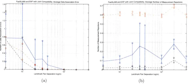
4.4.1 Interpretation of Data Association Results . . . .
4.4.2 Interpretation of Measurement Rejection Results . . . .
4.4.3 Filter Dependent Effects . . . .
. . . . 101
. . . . 103
. . . . 104
5 Results from Application of Filter-Data Association Marriages to Ex-perimental Data
5.1 Experimental Set-up ...
5.2 Limitations of FastSLAM 1.0 for the Car Park Data Set ...
5.3 Landmark Localization . . . .. . . . 5.4 Agent Localization . . . . 105 106 106 108 111
6 Conclusions and Future Work 115
List of Figures
1-1 Data Ambiguity as a Result of Measurement Uncertainty . . . 24
1-2 Data Ambiguity as a Result of Pose Uncertainty . . . . 25
1-3 Data Ambiguity as a Result of Landmark Uncertainty . . . 26
3-1 Joint Compatibility Branch and Bound Search for a two landmark - two
measurement scenario. . . . 57
3-2 Joint Compatibility as a Constraint Satisfaction Problem . . . 59
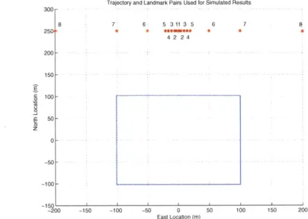
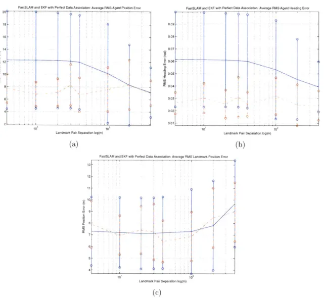
4-1 Trajectory and Landmark Pairings Used in Outside of Trajectory Case for Simulated Results. . . . 69 4-2 Performance of EKF and FastSLAM for Perfect Data Association Case
with Landmarks Outside of Trajectory . . . 70 4-3 Sequential Nearest Neighbor Data Association Performance Variation
Ver-sus Time and Landmark Separation for Landmarks Outside of Trajectory. . 73 4-4 Sequential Nearest Neighbor Data Association Measurement Rejection
Char-acteristics for EKF and FastSLAM where the Landmarks are Outside of the Trajectory. . . . 74 4-5 Average Measurement Rejection and Data Association Errors for
Sequen-tial Compatibility Nearest Neighbor using EKF and FastSLAM where the Landmarks are Outside of the Trajectory . . . .. . . . 75 4-6 EKF and FastSLAM performance using Sequential Nearest Neighbor Data
Association for the Case where Landmarks are Outside of the Trajectory. 76
4-7 Joint Compatibility Data Association Performance Variation Versus Time
4-8 Joint Compatibility Data Association Measurement Rejection Character-istics for EKF and FastSLAM where the Landmarks are Exterior to the
Trajectory. . . . . 79
4-9 Average Measurement Rejection and Data Association Errors for Joint Compatibility using EKF and FastSLAM where the Landmarks are Outside of the Trajectory .. . . 80 4-10 EKF and FastSLAM performance using Joint Compatibility Data
Associ-ation where the Landmarks are Outside of the Trajectory. . . . 81 4-11 Joint Maximum Likelihood Data Association Performance Variation Versus
Time and Landmark Separation for Landmarks Exterior to the Trajectory. 82 4-12 Joint Maximum Likelihood Data Association Measurement Rejection
Char-acteristics for EKF and FastSLAM where the Landmarks are Located
Out-side of the Trajectory . . . . t. . . . 84
4-13 Average Measurement Rejection and Data Association Errors for Joint ML where the Landmarks are Exterior to the Trajectory . . . 85 4-14 EKF and FastSLAM performance using Joint Maximum Likelihood Data
Association where the Landmarks are Exterior to the Trajectory. . . . 86 4-15 Trajectory and Landmark Pairings Used in Inside of Trajectory Case for
Simulated Results. . . . 90 4-16 Performance of EKF and FastSLAM for Perfect Data Association Case
with Landmarks Inside of Trajectory. . . . 91 4-17 Average Measurement Rejection and Data Association Errors for
Sequen-tial Compatibility Nearest Neighbor using EKF and FastSLAM with Land-marks Inside of Trajectory . . . 92 4-18 EKF and FastSLAM performance using Sequential Nearest Neighbor Data
Association with Landmarks Inside of Trajectory. . . . 93 4-19 Average Measurement Rejection and Data Association Errors for Joint
Compatibility using EKF and FastSLAM with Landmarks Inside of Tra-jectory . . . 94
4-20 EKF and FastSLAM performance using Joint Compatibility Data Associ-ation . . . 95 4-21 Average Measurement Rejection and Data Association Errors for Joint ML
with Landmarks Inside of Trajectory . . . ... . . 97 4-22 EKF and FastSLAM performance using Joint Maximum Likelihood Data
Association with Landmarks Inside of Trajectory. . . . 98
5-1 Path and Map Estimate Superimposed on GPS-Truth for Various SLAM
Filter-Data Association Marriages . . . ... . . . 109
5-2 Agent Localization Errors with Respect to GPS Path for Various SLAM
Filter-Data Association Marriages . . . 112
5-3 Root-Squared Agent Position Error with Respect to GPS Path for Various SLAM Filter-Data Association Marriages . . . 113
List of Tables
4.1 Pose, Landmark, and Measurement Uncertainties Used in Simulations . . . 67
4.2 Quantities Used in the Motion Model for the Simulations . . . . 67
4.3 Performance Comparison of Filter-Data Association Marriages for Agent Position Error for the Case where the Landmarks are Outside of the
Tra-jectory . . . . 87
4.4 Performance Comparison of Filter-Data Association Marriages for Land-mark Position Error for the Case where the LandLand-marks are Outside of the Trajectory . . . .. . . 88 4.5 Performance Comparison of Filter-Data Association Marriages for
Aver-age Data Association Errors Made for the Case where the Landmarks are Outside of the Trajectory . . . 89 4.6 Performance Comparison of Filter-Data Association Marriages for Agent
Position Error for the Case where the Landmarks are Inside of the Trajectory 99 4.7 Performance Comparison of Filter-Data Association Marriages for
Land-mark Position Error for the Case where the LandLand-marks are Inside of the Trajectory . . . 100 4.8 Performance Comparison of Filter-Data Association Marriages for Average
Data Association Errors Made for the Case where the Landmarks are Inside of the Trajectory . . . 101
5.1 Map Building Characteristics of the Various SLAM Filter-Data Association
Chapter 1
Introduction
The problem of robotic mapping, building a globally consistent of a robot's spatial
sur-roundings, becomes easier to solve if the true path of a robot is known
[40,
?]. At thesame time, if a perfectly accurate map of the robotic agent's surroundings is available then the problem of navigation, or localization, is easier to solve [8]. However, in most realistic applications involving mobile agents neither of these situations, the true path or map information, is available. Additionally, the environmental and motion measurements used by robots are noisy and this noise creates uncertainty in the system. The operation of these sensors correlates the uncertainty, and this correlation is what makes it possi-ble to simultaneously solve for both robot position and map of its surroundings [40]. This approach has come to be known as SLAM or CML, Simultaneous Localization and Mapping [9, 13] or Concurrent Mapping and Localization [25, 41], respectively.
One of the key issues in the SLAM problem is the data association problem [40]: decid-ing which noisy measurement corresponds to which feature of the map. Noise and partial observability can make the relationship between measurements and the model highly am-biguous. This problem is further complicated by considering the possible existence of previously unknown features in the map and the possibility of spurious measurements. The problem of data association in SLAM has recently received a great deal of attention within the Artificial Intelligence and robotics literature [3, 4, 31, 32, 21, 27, 28, 34]. Prior to this, a substantial amount of work had been done in the tracking domain, as in radar or target tracking [6, 5].
The data association problem is considered by some to be one of the hardest, if not the hardest problem, in robotic mapping [40] and a problem for which there exists "no sound solution" [39]. In particular, of the numerous data association algorithms that have been proposed in the literature it is not clear how these methods work with the various SLAM algorithms. Much of the recent literature on SLAM has emphasized the study of two types of filtering techniques: Extended Kalman Filters and Particle Filters, and the bulk of the research that has come out on data association emphasizes the use of one or the other of these SLAM algorithms. Different data association algorithms may have different effects on these filters, and it is the aim of this thesis to study these effects.
1.1
Why SLAM?
In situations where a robot, or even a human with a suite of instruments, is moving around an environment with the goal of both localizing itself and building up location information about its surroundings, e.g. mapping or target localization, the need for solving the SLAM problem becomes obvious.
However, utilizing a solution to the full SLAM problem may not be obvious in situa-tions in which an agent is concerned with only self-localization or target localization and map building: the question of whether or not solving the full SLAM problem is necessary when only a portion of the result is needed is of concern. In certain instances, such as those in which a reliable set of GPS signals are available, which are found in air-based systems or those that operate in open-field environments on the ground, solving the full
SLAM problem would not be necessary to maintain tightly bounded localization since an
external sensor eliminates the need for inference over robot pose. Unfortunately, there are numerous environments where good GPS signals are not available. For example, GPS signals are not available or dependable in urban canyon environments, which are found in most highly populated areas, as well as for most indoor environments.
Assume a situation in which an agent is operating in GPS-denied environments and its only concern is with self-localization. If it is not going to attempt to solve the full
Sys-tem (INS) such as accelerometers, gyroscopes, wheel encoders, doppler, or image based pseudo-inertial measurements. Even with the most accurate combinations of these de-vices, localization using on-line algorithms becomes difficult, as very small motion errors propagate themselves forward in time causing error growth. This problem along with the lack of state observability using only an INS will lead to a navigation filter that will eventually diverge; in other words the accuracy of the state estimate will quickly worsen
[10, 40]. In certain situations many of these problems can be alleviated, or at least
de-layed, by enforcing certain constraints on portions of the navigation filter. This topic is also discussed in reference [10].
If instead the goal of an agent is to only build a map or localize a target using relative
measurements, such as range and bearing, a map building solution may not even be pos-sible without knowing the robot's location. In situations where good a priori information is known, in regards to the robot's location, a solution to the map building problem can be attained. However, as soon as the robot begins to move around, the uncertainty in its location will begin to grow without bound for the previously mentioned reasons. Solving the SLAM problem is the logical resolution to these issues.
Further motivation for solving the SLAM problem is that it lends itself to use of instru-ments that are lightweight and cheap, as opposed to attempting to solve the mapping and localization problems separately which may in fact require more costly, complex instru-mentation (e.g. GPS). If implemented correctly a solution to the SLAM problem should be with a minimal amount of instrumentation. Additionally, solving the SLAM problem can be done in an autonomous fashion using online algorithms; therefore regardless of the user, be it robotic or human, it is anticipated that little or no user input will be required for use of an instrument suite that makes use of the correct SLAM algorithms.
1.2
SLAM Applications
There are numerous applications for which successful implementations of SLAM algo-rithms can be used to produce substantial benefits for both human and robotic agents. First, it is a prerequisite for successful operation of mobile robots in almost every realistic
situation [40], as most applications of mobile robots involve some form of a SLAM
imple-mentation. Some of the more interesting applications are found in undersea autonomous vehicles [33] and robotic exploration of mines [42], with additional possibilities of future application to extraterrestrial planet exploration [30]. For many of these applications the SLAM solutions are only used for navigation purposes, however some do make use of the created map information for future use [42].
In addition to robotics applications, SLAM solutions may be used to enhance the capabilities of humans in localization and mapping, which is potentially a very powerful concept. In particular, it is hypothesized that the correct implementations of SLAM solutions combined with the proper instrument suite should enable one to produce systems that could be used by humans, yet operate autonomously without human intervention. Such systems could be used in the place of those currently in operation that involve complex procedures to be useful and also require very heavy, expensive instrumentation. One example of this is found in the expensive and bulky equipment currently used by some U.S. military forces to localize targets at a distance using ground personnel.
These types of SLAM based systems could have numerous applications in the defense realm from forward operations involving the mapping of areas where future operation may occur, to tracking of future troop movements, and real-time mapping, as well as the localization of specific targets. The need filled by SLAM based systems would be for environments in which GPS signals either do not exist or are not dependable, such as the urban canyon or indoor environments.
Non-military related uses for these type of technologies may also exist in the areas of human extra-terrestrial planet exploration, as well as in terrestrial applications such as for use by sportsman or search and recovery teams where GPS signals are not useful or available.
1.3
SLAM Methods
There are many SLAM algorithms that exist in the literature at this point in time. Of these algorithms there are many different approaches for the various aspects of the
prob-lem. There are those that use a grid-based approach for representing the world such as
DP-SLAM [14, 15], as well as methods that attempt to describe the geometry of objects
in the map with various methodologies [44, 2]. Unfortunately, many of these method-ologies have serious limitations. For example, the DP-SLAM algorithm is formulated for use with a specific type of measurement device. In the case of the methods that attempt to describe the complex geometries of the environment, there is a tendency to have diffi-culty computing a solution in real-time especially for higher-dimensional or geometrically complex situations, i.e. numerous landmarks of various shape.
In the context of this thesis the methods considered will be those that maintain point representations of the world in continuous space, can be implemented as an online algo-rithm, have incarnations that scale well to high-dimensional problems, and can be flexible for use with any known type of environmental location measurements. From these con-straints the two SLAM solutions that will be considered are the Extended Kalman Filter and Particle filter, specifically Rao-Blackwellized Particle filters much like FastSLAM [30].
1.4
Need for Data Association Algorithms
Until recently much of the work on solving the SLAM problem neglected the data associ-ation issue by assuming that it was always known a priori for all measurements [40]. In any situation where the map of the world may contain more than one feature there will be some amount of data association ambiguity. In fact, even in the case where it is known that only one object exists in the world there will still be data association ambiguity if the possibility of spurious measurements is allowed. In most applications where SLAM solutions are used the number of dimensions required to describe the world is quite high, as the map must contain enough prominent features to sufficiently describe an agents surroundings. At the very least a minimal two-dimensional representation of an agent's environment would have on the order of magnitude 0(101) objects for a very simple prob-lem, as in the Car Park data set where the environment is made up of 15 unique features
or landmarks, along with the additional object of the agent itself
[1].
mea-surements, or assignment sets for multiple meamea-surements, is the ambiguity created by uncertainties in measurements, pose, and landmark locations. To effectively describe how each type of uncertainty leads to greater ambiguity in data associations, a number of figures will be examined. In these plots the following variables will be used: F denotes the corrent estimate of the location of feature i, Z is used to describe the measurement (or the location a measurement is indicating a feature to be), and St denotes the current estimate of the agent's pose.
Measurement uncertainty creates greater data association ambiguity since greater measurement uncertainty means a larger number of assignments must be considered. This occurs because more data associations will have non-negligible likelihoods, which is a metric used by many data association algorithms, see figure 1-1.
St
Figure 1-1: Data ambiguity as a result of measurement uncertainty. Here the inner dotted ellipse denotes a "small" measurement uncertainty while the outer solid ellipse denotes a "large" measurement uncertainty. Notice the increase number of features included within the measurement uncertainty with the larger value.
object(s) is being observed as it is not entirely certain where it is or where it is facing, as illustrated in figure 1-2.
+ Z9 +
FZ
F
2
Figure 1-2: Data ambiguity as a result of pose uncertainty. Here the ellipse surround-ing the "pose estimate" indicates the uncertainty in robot position, while the two dotted lines symmetric about the line pointing to the measurement indicate the heading uncer-tainty. This indicates that the pose and heading may be anywhere within this uncertainty,
therefore allowing for confusion of which feature, F or F2, the measurement should be
associated with
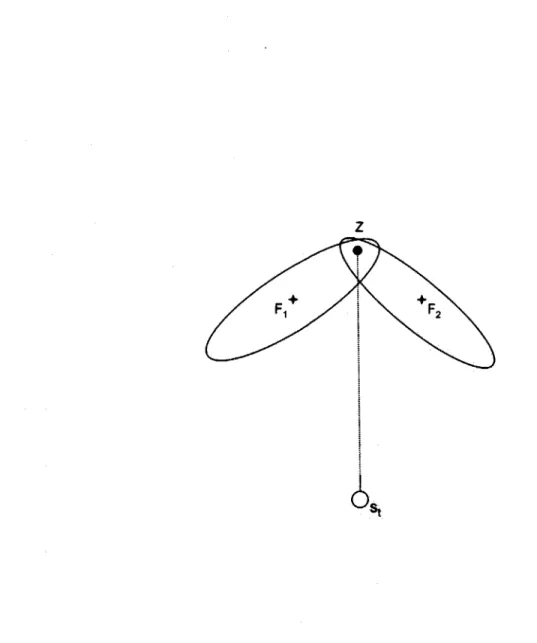
Finally, landmark uncertainty leads to assignment ambiguity by making it possible, in a probabilistic sense, for multiple measurements to be associated with a single measure-ment. This can be seen by the situation depicted in figure 1-3.
In practice all of these errors are usually affecting the agent all at once, in a super-position of errors. Additionally, it is often the case that each measurement must also be considered to be one of a never-before-seen object or of a spurious nature that must be removed. This combination of uncertainties makes data association very difficult.
Z
St
Figure 1-3: Data ambiguity as a result of landmark uncertainty. Here the uncertainty in
the location of features F1 and F2 makes it equally likely that the measurement Z should
1.5
EKF vs. Particle Filter Data Association
In this thesis, we will look at two particular inference algorithms, each with an inherently different treatment of the data association problem. In the EKF a single data association is used for each measurement in a very stiff manner, such that the assignment hypothesis made at the current time cannot be altered in the future, if future information indicates it was incorrect. This is a result of the EKF committing to an a posteriori distribution over robot poses and landmarks that is maintained as a single unimodal Gaussian.
In contrast, the Rao-Blackwellized particle filter represents the posterior over poses and landmarks non-parametrically, sampling particles from the posterior. The FastSLAM 1.0 particle filter allows for per-particle data association, thereby allowing for consideration of M independent data association hypotheses where M is the number of particles used in the filter. Since the uncertainty in the states is carried along in the dispersion of particles and their map knowledge as opposed to a covariance matrix, the effect of data association assignments differs substantially from the EKF. Finally, the operation of this particular method is such that with a non-zero probability the filter will eliminate those particles, or hypotheses, that have made incorrect data correspondences. This fact has the potential to have the greatest impact on the way ambiguous data associations will affect it.
1.6
Data Association Methodologies
A number of data association methodologies have been proposed and studied in the SLAM
literature. It has generally been the case that these methods have only been applied to either EKF or FastSLAM without direct comparisons being made between the two. One such method that was recently proposed is known as Joint Compatibility (JC) and was applied to an EKF SLAM solution [31, 4]. In the original paper [31] that proposed this method it was compared to another data association algorithm Sequential Compatibility
Nearest Neighbor (SCNN); however it too was only applied to an EKF implementation.
The majority of the first papers to explore the FastSLAM algorithm used a maximum likelihood approach for data association [30, 28, 45], while one paper also explored a
particle splitting method of data association for FastSLAM [34]. However, none of these papers mentioned above explore the performance of both EKF and FastSLAM using the same data association methods.
Another data association method for SLAM that has been proposed in the literature,
is Combined Constraint Data Association (CCDA), which is formulated and explored in
[4]. However, according to [30] this methodology should perform similarly to JC with the additional property that it can be used to determine pose information if none is available
a priori.
One additional method that is mentioned in [30] is the concept of randomly sampling data associations on a per-particle basis. As mentioned in this reference the sampling would be done from a Probability Mass Function, or PMF, as defined by the normalized likelihoods of measurement associations. It would of course be possible to sample from some other PMF if so desired. While this method makes some intuitive and even mathe-matical sense for the FastSLAM formulation, it is unclear if this method would be a useful approach for the EKF.
There are other data associations that have recently been mentioned in the literature that involve the use of the Hough Transform and the RANSAC algorithm. These methods, as discussed in the available literature, perform data association in a delayed manner. In doing this there are some possible gains in data association performance, however the end result is that measurements will not be processed in real-time.
1.7
Thesis Statement
It is the intention of this document to advance the following thesis:
"The performance of a given data association algorithm for SLAM, in terms of the propensity of data association errors made and the subsequent effect on localization and mapping accuracy, depends on whether it is used in conjunction with an Extended Kalman Filter or a Rao-Blackwellized Particle Filter formulation as the solution to the SLAM problem."
1.8
Thesis Overview
The research done in this thesis can be described by the following items:
- Three batch data association algorithms will be examined and described in detail:
Sequential Nearest Neighbor, Joint Compatibility, and Joint Maximum Likelihood
- The operation of the three data association algorithms will be studied with regards
to their operation when married to both EKF and FastSLAM filter implementations.
- The performance of the SLAM filter-data association combinations will be examined
Chapter 2
Simultaneous Localization and
Mapping
The Simultaneous Localization and Mapping, or SLAM, problem first arose when it was recognized that problems of robotic mapping and navigation are very difficult, and in some situations impossible, to solve as separate problems. The methods that have been the most successful in solving the SLAM problem have been ones that make use of sta-tistical methods for taking into account the uncertainty in the system states as well as measurement uncertainty. Such a method was first proposed and popularized in a serious of seminal papers by Smith, Self, and Cheeseman [37, 38] in which the solution took the form of the Extended Kalman Filter.
Solutions to the SLAM problem can be very effective in situations when global mea-surements such as GPS are not available, for instance in the case when a robot or agent that operates indoors or in the urban canyon. In these situations, the uncertainty in both the location of objects in the environment as well as the robots own pose become tightly linked. This is due to the fact that in these situations the agent must rely on relative measurements relating its current pose with objects in its surroundings, such as range and bearing measurements. This is what leads to the concept of solving the Simultane-ous Localization and Mapping or SLAM problem, which has also been called Concurrent Mapping and Localization, or CML, in the literature [32].
2.1
Extended Kalman Filter SLAM
Framing the SLAM problem as a partially observable Markov chain allows for a compact, probabilistic notation of the SLAM problem which is known as the Bayes Filter Equation and is derived from the SLAM posterior [30]. For the Bayes Filter equation and the SLAM posterior to be true statements, the Markov assumption must hold. This assumption states that if the current state is known then the previous and future data are conditionally independent [11]. By making some very restrictive assumptions, the Bayes Filter equation will be equivalent to a Kalman Filter [39, 30].
In order to describe this problem a number of variables must be defined. First, the
states of the system are represented by st the robot pose at time, t, and
e
the locationof the objects in the environment that are known to the robot, which is also referred to as the map. The robot pose consists of N, the agent North position, Eag the agent East
position, and 0,g the agent heading. The map information,
E,
as it exists within thestate vector consists of the North and East positions of all landmarks in the environment,
NIN and EIN respectively for the N-th landmark. The environmental measurements as
considered across time are given by z' = {zo, zi, ..., zt} and the motion measurements
or controls as taken over time are given by w = {wo, w1, ..., Wt}. The quantity 7 is a
normalization constant that is a byproduct of applying the Bayes rule.
What we wish to maintain at each time, t, is a distribution over the current robot pose and landmarks. We call this the SLAM Posterior:
p(st,
e|zt,
wt) (2.1)Using Bayes Rule this can be re-written as:
p(st,
EIzt,
wt) = 7 -p(ztlst,E,
z Wt) .p(st,Izt-l
Wt) (2.2)After some manipulation this can be converted into the Bayes Filter Equation:
This is a tractable formulation because it allows us to compute p(st,
elzt,
wt)recur-sively, from the known sensor model p(ztlst, 0), the known motion model p(stlst_1, wt), and the SLAM posterior of the previous time step p(st_1, |ztl-, wt-). In the filter formu-lations discussed here, the landmarks are thought of as point objects with single locations in two-dimensional space, such as the corner of a building or the center of a small tree. While this is an approximation, it is sufficient for the purposes of the algorithm develop-ment discussed here. Additionally, the error in this approximation can, for the most part, be absorbed in measurement error and uncertainty in feature locations.
2.1.1
The EKF Formulation
The SLAM problem can easily be framed as a state space system and therefore fits into the Kalman filter framework. In real-world applications there are often non-linearities involved in the physics of the situation, which is why the EKF is used. This formulation is essentially the same as the traditional Kalman filter architecture with linearization performed to allow for the real world physics of the system dynamics and the measurement models.
The solution offered by the EKF is attained by assuming a multi-variate Gaussian distribution used to describe p(x). In addition the noise in the IMU and environmental measurements must be assumed to be white. Finally, it also assumes that substantial errors are not incurred by making use of linear approximations of the dynamics of the state propagation in time, as well as in the physics of the state relationships for environmental measurements.
The building blocks of the EKF are the state vector and its associated covariance matrix.
x = t (2.4)
Nag St Eag (2.5) #ag (2.6) N, Ell E =(2.7) NN E N
Then the covariance matrix is defined as:
2
Nag NagEag ''' ''' ''' UNagEIN
2 - -O"NagEag UEag 2 qOag U2 ... g.. ... ... ... 2 LNagEN ''' '' E1N
-In general this matrix is initialized as a diagonal matrix, where the variances which lie on the diagonal represent the a priori knowledge with regard to the uncertainty in the individual states, which consist of features and the robot pose. The off-diagonal terms are built up over time by the filter and represent the correlations between these filter states. Finally, knowledge of the measurements being considered by the filter must be un-derstood. This includes both a model of the physical measurements, as well as the noise characteristics of these measurements. To be consistent with what is used throughout the analysis done here, range and bearing measurement pairs will be considered as a simultaneous measurement of a single landmark. This is a reasonable for a number of instruments that are used in SLAM implementations, such as the SICK laser.
The physical measurements for the range and bearing can be represented as:
hk(x)=
(Nij(k) - Nag(k)) 2 + (Ej(k) - Eag(k)) 2
arCtan Ni.(k)-Nag(k)) ag
I
(2.9)
However, the actual measurement is noisy and is modeled in the following way:
Zk(X) = hk(X) + Uk (2.10)
Where the noise is represented by the vector of random variables Uk, which is
zero-mean gaussian white noise.
Uk- ~N(0, Rk) (2.11)
The knowledge of the measurement uncertainty is represented by the measurement
covariance matrix, Rk.
F
21
R= r 0rb 2[
rb UbJ (2.12)The motion model used is very simple: it is assumed that the robot issues controls of translational and rotational velocity in two-dimensions.
Vk-1 = Vtrue + Wv,k-1
Ok-1 = Qtrue + WS,k-1
(2.13)
(2.14)
Wk1 =
[
Wvk1 N(O,Q)
(2.15) [W,k-1Q
=V
(2.16)0 g02
Now the operation of the EKF formulation can be laid forth, where Zk represents the
actual measurement received and sk represent the estimated measurement as determined
by the current values of the state estimate xk [18, 22].
Propagation Step:
1. Propagate the state estimate in time:
ik(--) = q(2k-1(-), Vk_1, (-1) (2.17)
Where k - 1 indicates the most current information available for that variable.
2. Propagate the state covariance matrix: 1
Pk(-) = k_1Pk-1(+)D_1 + GkQG _ (2.18) cos(Oag,k-_) 0 sin(qag,k-_) 0 0 1 Gk_ = 0dt (2.19) 0 0
o
o
Here, the quantity dt is the time step over which state propagation is occurring. The state transition matrix, b-1, is defined for this case as
'This equation is the result of the following derivation, where the (-) terms have been dropped for sim-plicity. Here, Xk is the truth state and ik is the filter's estimate of the state: z4 = Xk - 4 = error in state estimate, Pk = E[zz], and ik = (=I-izk_1 -Gk-1wk-1)(k-1_1k- -Gk-_wk_1) T
. After
eliminat-ing terms that go to zero, this can be rewritten as: z4z = Dk-ikz-i 1_k1 + Gk_1wk_1wkj_1G_,
4k-1 k = - 4) = I(2N+3)x(2N+3) (2.20)
an identity matrix of size (2N +3) x (2N +3) since there are no states carried along that explicitly describe the dynamics of theworld, i.e. velocity or acceleration states. Measurement Update Step:
1. Covariance matrix update:
Pk(+) = [I - KkHk]P(--) (2.21)
Kk Pk(-)Hkj[HkPk(-)Hj + Rk] (2.22)
The matrix Hk, known as the measurement matrix, is the Jacobian of the
measure-ment model hk (x).
2. State estimate update:
k(-) = Xk(-) + Kk[zk - (k] 2.23)
Hk = Vhk(X) - hk(x)
HD =hXk) =(2.24)iox Lk
2.1.2 Major Issues on the Use of EKFs for SLAM
One of the major road blocks that has faced the EKF method in its application to so-phisticated problems has been the growth in complexity of the filter with the number of objects in its map. This is primarily due to the fact that this method, in its original
formulation, relies on a covariance matrix of size O(N 2), where N is the number of objects
in the map.
There has been significant effort within the AI community to address this problem during recent years. One method which has been shown to resolve the complexity issues surrounding the use of EKF formulations and is considered the current state-of-the-art by many, is known as Atlas [7]. This method promises constant time, or at least bounded
time, operation and is therefore not dependent on the size of the map. However, it should be noted that the use of the Atlas methodology is not limited to EKF solutions of the
SLAM problem, because in its general form it is a framework for using filtering methods
that aims to reduce complexity, rather a filtering method itself. There are other EKF related methods which also promise either constant time or improved time operation and have been shown to produce good results, such as Sparse Extended Information Filters (SEIFs) [43, 27] and compressed EKFs [19, 20].
While these approaches do address computational limitations of the EKF formulation they do not, in their basic formulations, fully address the data association problem. The implementation of these methods and their robustness to data association errors will not be discussed in this thesis since there is no evidence in the literature, as well as no logical reason to believe otherwise, that these methods would be more robust to data association errors than the traditional EKF-based SLAM approach.
2.2
Particle Filter SLAM
Particle filters consist of a large class of Monte Carlo estimation methods that are ap-plicable to problems that can be posed as partially observable Markov chains [39]. The formulation of the particle filter has been around since the mid-to-late 1990's, originally proposed in papers by Kitagawa as well as Liu and Chen [24, 26]. Indeed the applica-tions of particle filters to robotics problems are very widespread, but some of the greatest achievements made by their use comes in the area of localization and mapping. The particle filter is credited with having solved the global localization and the kidnapped robot problem, both of which were previously unsolved and considered to be important for robust mobile robot operation. [39].
One of the greatest drawbacks of the particle filter, as it was originally formulated, is that it does not scale well to high dimension state spaces. This is a result of the exponential time behavior of this implementation of the particle filter, which is not acceptable for problems such as SLAM which must be solved in real-time while maintaining numerous states. A development in the literature that has offered some resolution to this problem
is the Rao-Blackwellized particle filter [12]. This method has not only showed promise to greatly increase computational efficiency, but also improve estimation accuracy. The concept of a Rao-Blackwellized particle filter for application to the SLAM problem has been greatly developed in a number of papers by Montemerlo and Thrun [28, 29, 45, 30].
2.2.1
Particle Filter Advantages
Particle filters have a number of useful properties when compared to other methodologies for solving the SLAM problem, such as the EKF. First, the particle filter can approximate arbitrarily complex probability distributions, where as the EKF is restricted to Gaussian descriptions at all levels of uncertainty. Additionally, particle filters are not adversely affected by significant non-linearities in the motion and measurement models. This is because linearization is not required in the propagation of the state uncertainty, as this information is carried along in the distribution of the particles.
2.2.2
Particle Filter Formulation
For application of particle filters to the SLAM problem it is possible to begin at the same place as was done for the EKF formulation, that is the SLAM posterior.
p(st, EztI, wt) (2.25)
As in the Kalman Filter formulation, this probabilistic relationship is valid if the Markov assumption holds. The Markov assumption states that if the current state is known then the previous and future data are conditionally independent [11].
As was done previously for the EKF the SLAM posterior can be converted into the Bayes Filter equation by use of the Bayes Rule.
p(stIzt, wt) = 'r -p(ztIst,
E)
-fp(st, 8|st_1, 1 1 wt-1) p(st_1z~1, wt)dst_1 (2.26)ap-proximating the continuous probability densities defined in equation ( 2.26) with discrete samples. The SLAM posterior may be thought of as a belief state, where a single belief (i) is defined as a hypothesis of agent pose, the map of the environment, and an associated weighting that defines the probability of the given belief being correct. In the particle filter this is represented by M samples of a continuous probability distribution along with the associated weighting for each sample.
belief (i) = p(st(i),
E(i)|z1(i),
w'(i)) = {st(i), ( i)}i-1...,m (2.27)At initialization this belief state, belief (i), is defined by whatever probability distrib-ution is known to define the uncertainty in st and
E
[11, 39].p(so,
EIz
0, wO) = p(so,E)
(2.28)
First, if a priori information describing the uncertainty in the states is available it is used to define the initial distributions. These distributions are then sampled from, to
create the particle representation of the state space x0(i), po(i), where po(i) is the particle
weighting. The particle weighting is generally initialized to [11].
The estimation of the posterior can then be done in the following recursive fashion:
1. Propagation Step:
Obtain the new pose st(i) using p(stlst_1, wt_1) where this is equivalent to
propagat-ing each st-1 uspropagat-ing independent samples of wt_1. This is defined by a motion model.
St(i) = g(st_1(i), wt_1(i)) (2.29)
Here, the variable wt_1 represents the noisy motion information of the agent as in equations 2.13 and 2.14, however in this case the noise can be represented by any probability distribution that can be sampled from. This process approximates the following predictive density:
U __________________ _____
p(stlsti, wt_)p(st_1, 6|ztI, wt~l) (2.30)
2. Measurement Step:
Now alter the belief state by weighting the particles using the likelihood of the particle occurrence given the measurement, zt.
p(ztIst(i), E) (2.31)
3. Re-sample Step:
Re-sample the M particles with replacement based on the normalized weighting, where
M
ZP(i) = 1 (2.32)
i=1
Loop back to step 1.
This procedure approximates the creation of the following posterior probability dis-tribution [11].
p(ztjst,
e)p(stlwt_1,
st1)p(sti, |z- 1, wt-1)(2.33)
p(ztlzt-1, wt_1)
Note, that in actuality the distribution that would be ideal to sample from is the
desired posterior, p(st,
Ezt,
ut), however this target function is unavailable. Using thisratio to determine the particle weighting along with the sampling procedure described in the section above, allows for the creation of an approximation to the desired posterior. This procedure is an example of a sampling importance re-sampling (SIR) algorithm [35].
2.2.3
Rao-Blackwellized Particle Filter
The Rao-Blackwellized particle filter is a variation of the traditional particle filter that scales well to problems of higher dimension. The Rao-Blackwellized particle filter is very general in its formulation and can be applied to problems other than SLAM [17, 23]. However, the formulation discussed here will only explore this type of filter as it applies
to the SLAM problem, in particular the incarnation known as FastSLAM 1.0 will be discussed [45]. In the FastSLAM formulation, a slightly different form of the SLAM posterior is used then what was presented in sections 2.2.2 and 2.1.1:
p(St
EIz',
w', n') (2.34)The differences exist in the variable s' = {SO, Si, ..., st} which represents the entire robot path (not just the current pose) and the variable nt = {fno, ni, ..., nt} which represent
the correct data associations over all time. The reason for maintaining the entire path,
St, in the equation will be explained below. However, the presence of the data association
assignment vector in the formulation does not seem to be dealt with in a satisfying manner in this formulation.
The formulation invokes the Rao-Blackwellization concept of marginalizing out vari-ables from the posterior equation by implementing the proper conditioning. This was first developed in [12] to factor the SLAM posterior into the following:
N
p(st, E)zt, wt, nt) = p(stjzt 7 Wt ,nt e Ist, zt, ut, nt) (2.35)
i=1
In words this means that it is possible to factor the problem into N+1 estimators.
The first estimator represented by p(stIzt, w, nt) aims to determine the posterior of path and the other estimators p(E|st, zt, ut, nt) are used to determine the location of the N landmarks.
The path posterior p(stlzt, wt, nt) is estimated using a particle filter. The landmark estimators are obtained using EKFs, where each particle of the FastSLAM filter maintains
N independent Kalman filters for estimating the N landmarks. The independence of the
EKFs are a result of conditioning each landmark estimator on the robot path. This has the benefit of only having to maintain N 2 x 2 covariance matrices for each particle as opposed to a full (2N + 3) x (2N + 3) covariance matrix.
The result is a set of particles where the i-th particle is defined as:
Here each particle contains a path along with the mean, ym,t(i), and covariance matrix,
Pm,t(i), for each of the N landmarks the particle is trying to estimate the location of, using an EKF.
For initialization the pose portion of the particles is found in a manner similar to that of the traditional particle filter.
p(so1z0, wo, no) = p(s0) (2.37)
Therefore the initial particles are sampled from the pose probability distribution de-fined by the available a priori information.
Using this framework the operation of the FastSLAM filter is now very much the same as that laid out in the section on particle filters 2.2.2. Here the aforementioned weight is calculated as follows [45].
pA~i) - targetdistribution p(st(i)|zt,wt,nt)
proposaldistribution p(st(i)|I-1,w, nt-1)
In actuality the distribution that would be ideal to sample from is the desired posterior,
p(stIzt, u', nt), however this target function is unavailable. Using this ratio to determine
the particle weighting along with the sampling procedure described in the section on particle filters, allows for the creation of an approximation to the desired posterior. This procedure is an example of a sampling importance re-sampling (SIR) algorithm [35].
Using the Bayes Rule and a Markov assumption the weighting function can be written as [30].
pt(i) = p(ztst (i), zt4~1 wt, nt) (2.39)
This form allows for advantage to be taken of the EKF form of the landmark estimator. Now the weight per-particle can be written as the likelihood function for the measurement.
pt(i) = exp - -_(z nt,'t)Zt(Zt - (2.40)
Chapter 3
Data Association
The problem of data association refers to the concept of relating the states of nature from which a measurement or set of measurements originate. There are many applications when data associations are known a priori or the problem of choosing the correct ones becomes trivial. However, for the problem of autonomous agents attempting to solve the
SLAM problem it is a key component. In fact it is one of the most difficult aspects of
developing a full solution to the SLAM problem [40, 4].
The study of data association has historically received the most attention within the literature on target tracking [5, 6]. However, with increasing attention in recent years being given to obtaining full solutions to the SLAM problem for robotic agents there has begun to be increasing attention to the data association problem within the Al literature
[31, 3, 32, 21, 27, 4].
Much of the work that has come out of the AI/SLAM literature has sought to apply the ideas previously laid out in the tracking literature to the SLAM problem. At the same time some approaches to data association that have come out more recently appear to be unique to the SLAM domain such as maximum common subgraph (MCS), combined
constraint data association (CCDA), and to a lesser extent joint compatibility branch and bound (JCBB) [4, 3, 31]. None-the-less many of these approaches have been demonstrated
to perform successfully under specific conditions and implemented with particular data association-SLAM filter pairings.
comparison of the performance of the most prevalent of these algorithms. In particular, how these algorithms perform when paired with the most popular filters for solving the
SLAM problem and if the various data association picking algorithms will perform the
same independently of the filter they are paired with.
3.1
Individual Measurement Data Association
The simplest form of the data association is that of having to associate a single mea-surement with the appropriate feature in the environment, where this could also include the possibility of either a spurious measurement or a previously unknown feature. This form of the problem, as opposed to a set of batch measurements that can be considered as being received simultaneously, appears to be very common in the tracking literature, from which many of the data association ideas originate.
3.1.1
Maximum Likelihood
One of the most basic and simplest methods for performing data association is to con-sider the measurement likelihoods. This is done by calculating the likelihood that each landmark known to the agent, i.e., that exists in the SLAM filter, is associated with the in-dividual measurement being considered. This method is also known as Nearest-Neighbor data association in the literature [5].
In general the likelihood or Nearest-Neighbor calculation can be made for any prob-ability distribution, as long as the probprob-ability density can be calculated for any possible measurement. For every case considered in this thesis the following assumptions will be made, thus allowing for a straightforward analytic representation of the likelihood.
- The true measurements at the present time are normally distributed, i.e. the
measurement noise is gaussian.
- A priori knowledge of the characteristics of the measurement noise is available in
terms of standard deviation omeasure and the mean.