Taming Private Leviathans : Regulation versus Taxation

(1)

HAL Id: hal-03129746

https://hal.uca.fr/hal-03129746

Preprint submitted on 3 Feb 2021

HAL is a multi-disciplinary open access archive for the deposit and dissemination of sci-entific research documents, whether they are pub-lished or not. The documents may come from

L’archive ouverte pluridisciplinaire HAL, est destinée au dépôt et à la diffusion de documents scientifiques de niveau recherche, publiés ou non, émanant des établissements d’enseignement et de

Grégoire Rota-Graziosi, Islam Asif, Rabah Arezki

To cite this version:

Grégoire Rota-Graziosi, Islam Asif, Rabah Arezki. Taming Private Leviathans : Regulation versus Taxation. 2021. �hal-03129746�

(2)

S U R L E D E V E L O P P E M E N T I N T E R N A T I O N A L

SÉRIE ÉTUDES ET DOCUMENTS

Taming Private Leviathans:

Regulation versus Taxation

Rabah Arezki

Asif Islam

Grégoire Rota‐Graziosi

Études et Documents n°5

January 2021

To cite this document:

Arzeki, R., Islam, A., Rota‐Graziosi G. (2021) “

Taming Private Leviathans: Regulation versus

Taxation”, Études et Documents, n°5, CERDI.

CERDI POLE TERTIAIRE 26 AVENUE LÉON BLUM F‐ 63000 CLERMONT FERRAND TEL. + 33 4 73 17 74 00

(3)

The authors

Rabah Arezki

Chief Economist, African Development Bank, Senior Fellow, Harvard Kennedy School of

Government, Research Fellow, Université Clermont Auvergne, CNRS, CERDI, F‐63000 Clermont‐

Ferrand, France

Email address:

r.arezki@afbd.org

Asif Islam

Senior Economist, Chief Economist Office of the Middle East and North Africa, World BanK

Email address:

aislam@worldbank.org

Grégoire Rota‐Graziosi

Director of Centre d’Etudes et de Recherche sur le Développement International, Professor in

Economics, Université Clermont Auvergne, CNRS, CERDI, F‐63000 Clermont‐Ferrand, France

Email address:

gregoire.rota‐graziosi@uca.fr

Corresponding author: Rabah Arezki

This work was supported by the LABEX IDGM+ (ANR‐10‐LABX‐14‐01) within the program “Investissements d’Avenir” operated by the French National Research Agency (ANR).

Études et Documents are available online at:

https://cerdi.uca.fr/etudes‐et‐documents/

Director of Publication: Grégoire Rota‐Graziosi

Editor: Catherine Araujo‐Bonjean

Publisher: Aurélie Goumy

ISSN: 2114 ‐ 7957

Disclaimer:

Études et Documents is a working papers series. Working Papers are not refereed, they constitute research in progress. Responsibility for the contents and opinions expressed in the working papers rests solely with the authors. Comments and suggestions are welcome and should be addressed to the authors.

(4)

3 Abstract

This paper explores the interplay between top wealth and policies namely regulation and

taxation exploiting variation in exposure to international commodity prices. Using a global panel

dataset of billionaire’s net worth, results point to a positive relationship between commodity

prices and the concentration of wealth at the top. Regulation especially pertaining to competition

is found to limit the effects of commodity price shocks on top wealth concentration while

taxation has little effect. Moreover, commodity price shocks crowd out non‐resource tax revenue

hence limiting the scope for income transfers and redistribution. Results are consistent with the

primacy of ex ante interventions over ex post ones to address top wealth inequality.

Keywords

Inequality, Wealth concentration, Competition, Tax, Natural resources, Development

JEL Codes

D31, D63, H26, H20, 013

Acknowledgments

We thank Andrea Barone, Olivier Blanchard, Simeon Djankov, Daniel Lederman, Tarek

Masoud and Lemma Senbet for excellent suggestions and comments. We acknowledge the

support received from the Agence Nationale de la Recherche of the French government through

the program “Investissements d’avenir” (ANR‐10‐LABX‐14‐01). The findings, interpretations, and

conclusions expressed in this paper do not necessarily reflect the views of the CERDI, World Bank

or the African Development Bank or the governments they represent. The CERDI, World Bank

and the African Development Bank do not guarantee the accuracy of data included in this work.

(5)

“Any contract… in restraint of trade” and “Every person who shall monopolize, or attempt to monopolize…shall be deemed guilty of a felony” – US Sherman Act (1890)

1. Introduction

In the late 19th century in the United States, rising inequality, social tensions and oligarchy led the federal government to reinvent itself as a regulator. The Sherman Antitrust Act of 1890 is the foundational federal

statute in the development of U.S. competition law.1_{At the time, the gilded age called for a forceful response}

by the federal government to curb the rising power of the so-called robber barons including Cornelius Vanderbilt, John D. Rockefeller and Andrew Carnegie. Fast forward to today the global rise of a class of billionaires coupled with heightened social tensions raise important questions about what to do about top wealth and income inequality (Wu, 2018). Competition policies and antitrust laws combined with strong enforcement mechanisms have a potentially powerful role to play in shaping the structure of an economy and society over and beyond taxation and redistribution policies. Indeed, protected sectors, cartels or

collusion limit the impetus for investment, innovation, and growth (see Aghion and Griffiths, 2005). The

present paper explores the interplay between top wealth and policies namely regulation and taxation exploiting variation in exposure to international commodity prices.

The rise of top income and wealth inequality over recent decades is a consistent pattern across the world (Piketty, 2014).2_{Initially the rise of top incomes was documented for the United States and France (Piketty}

and Saez, 2003; Piketty, 2003), followed by several other advanced economies (Atkinson et al., 2011). Studies on top incomes in developing economies is sparse due to data limitation, but several studies have documented top income trends in developing economies.3_{The rise of top incomes points to a number of}

concerns including significant welfare losses for workers and associated adverse political consequences (Alesina and Perotti, 1996; Bartels, 2008; Lansing and Markiewicz, 2016). Wealth concentration at the top also raises issues regarding policies including as to whether interventions should be ex ante or ex post (Fleurbaey and Peragine, 2013; Hsu, 2014).

The jury is still out on what drives the rise of top incomes. The literature has identified several factors driving top income and wealth inequality namely globalization, technology, labor market institutions, decline in competition and fiscal policy—or generally social norms regarding pay inequality (Ma and Ruzic, 2020; Piketty and Saez, 2003; Philippon, 2019; Aghion et al, 2019). Hsu (2014) argues that there are legal roots to top income inequalities which might explains the pervasive higher returns to capital compared to the rate of GDP growth. On the normative front, there is a heated debate on the best approach to address the rise in top incomes. The dominant approach is either to address institutional factors favoring the ability of top income earners to channel rents their way or to reduce the returns to rent seeking by increasing

1_{The Sherman Act gave way to The Clayton Antitrust Act of 1914.}

2_{Notwithstanding the conceptual differences between wealth and inequality, the two terms are used interchangeably}

thereafter. In the present paper, we use a measure of wealth inequality. As such the focus of the paper is on latter. In practice, measure of income and wealth inequality are strongly correlated. What is more, data on top incomes using tax administration data are more readily available than top wealth.

3_{For studies of wealth and income inequality in developing countries see Banerjee and Piketty, 2005; Leigh and van}

(6)

marginal rates of taxation on high incomes (Bivens and Mischel, 2013). More recently a debate has been raging on the use of a wealth tax as an instrument to reduce top incomes (Saez and Zucman, 2019).4

In this paper, we document that different institutional arrangements lead to a differentiated effect of (plausibly) exogenous commodity price fluctuations on top incomes.5_{To do so, we combine a global panel}

dataset from Forbes Magazine on billionaires’ net worth with an index of (country specific) commodity terms of trade shocks. Commodity shocks are significant sources of macroeconomic variation but also have important sectoral implications which elucidate linkages with concentration of income at the top. Results show that commodity booms lead to top income concentration, and the effect is economically large. Figure 1(a) globally traces the patterns of commodity shocks and the log differences of billionaire net worth and shows that they co-move. Figure 1(b) replicates the same pattern for developed (left panel) and developing economies (right panel) and shows the positive relationship between commodity price shocks and top incomes stand, regardless of the level of development. This finding is robust to accounting for sector of activity as well as the individual characteristics of billionaires as captured by billionaire fixed effects. The evidence is also suggestive that competition policy weakens the relationship between commodity booms and top incomes, and tax policy has no effect. However, we do find that commodity booms tend to lower tax revenues in the economy hence reducing the scope for income transfers and redistribution.

In addition to the literature on top incomes, this paper contributes to several strands of literature. Specifically, the paper also relates to the so-called “resource curse” literature. The latter has provided (mixed) empirical evidence that countries with large dependence in natural resource grow slower (see survey by Ross et al., 2015) and are also more unequal (Ross, 2001; Sokoloff and Engerman, 2000).6

Importantly, Mehlum, et al (2006) provides evidence that the effect of natural resources on the economy depend on quality of institutions.Furthermore, the type of natural resource matters with hydrocarbon and mineral resources, categorized as “point source” resources, having a more detrimental impact on growth than “diffuse” resources such as agriculture (see Isham et al., 2005). We contribute to this literature by focusing on the top incomes as opposed to general income inequality while exploring the role of different policy/institutional frameworks. We also find that commodity price shocks emanating from point source lead to more top income concentration than shocks stemming from diffuse resource.

4_{See debate hosted by the Peterson Institute for International Economics:}

https://www.piie.com/events/combating‐inequality‐rethinking‐policies‐reduce‐inequality‐advanced‐economies, accessed May 16, 2020.

5_{To the extent that commodity prices and stock markets comove, changes in commodity prices also affect} billionaires’ net worth through changes in stock market valuation. See Arezki, Loungani, van der Ploeg and Venables (2014) and Ing-haw Cheng and Wei Xiong (2014) for a discussion on the respective role of fundamentals and financialization in driving commodity price fluctuations.

(7)

Figure 1a: Log Differences of Billionaire Net Worth and Commodity Shocks

Figure 1b: Log Differences of Billionaire Net Worth and Commodity Shocks – Developing vs Developed Economies

Sources: Forbes Magazine (2001 to 2018); Gruss et al. (2019).

Globalization has led to a significant decrease in the cost of international capital mobility. In turn, this has fueled intense tax competition, which offers multiple opportunities to shift profits or wealth in tax

accommodating countries or tax heaven. Any tax coordination at the international level is rendered difficult or nearly impossible (see Rota-Graziosi, 2019). This may explain why taxation appears less efficient than regulation to tame top wealth inequalities as in this paper. Alstadsæter et al. (2018) finds that 10 percent of world wealth is held in tax havens and that this mask important heterogeneity. Andersen et al. (2017) finds that around 15% of the windfall gains accruing to petroleum-producing countries with autocratic rulers is diverted to secret accounts. The emerging debate on curbing top incomes has centered around the wealth tax (Saez and Zucman, 2019). There is indeed a strong theoretical case for a wealth tax especially after calamities such as wars and pandemics, yet its implementation and

‐0,02 ‐0,015 ‐0,01 ‐0,005 0 0,005 0,01 0,015 ‐0,6 ‐0,4 ‐0,2 0 0,2 0,4 2001 2002 2003 2004 2005 2006 2007 2008 2009 2010 2011 2012 2013 2014 2015 2016 2017 2018 Lo g d ifference of commodit y N et Exp o rt Pric e In d ex Log d ifference o f B illi on aire N et Wor th Years

Global

Log difference of Billionaire Net Worth Log difference of commodity Net Export Price Index (historic rolling weights) ‐0,02 ‐0,015 ‐0,01 ‐0,005 0 0,005 0,01 0,015 ‐0,6 ‐0,5 ‐0,4 ‐0,3 ‐0,2 ‐0,1 0 0,1 0,2 0,3 0,4 Lo g D if fe re nc e o f C om m o di ty N et Ex p or t P ri ce In de x Log D if fe re nce o f B ill io na ire N et Wo rt h Developed Economies Log difference of Billionaire Net Worth Log difference of commodity Net Export Price Index (historic rolling weights) ‐0,025 ‐0,02 ‐0,015 ‐0,01 ‐0,005 0 0,005 0,01 0,015 ‐0,6 ‐0,4 ‐0,2 0 0,2 0,4 0,6 2 001 ₂002 ₂003 ₂004 005₂ ₂006 ₂007 ₂008 ₂009 ₂010 ₂011 ₂012 ₂013 014₂ ₂015 ₂016 ₂017 ₂018 Lo g D if fe re nc e o f C om m o di ty N et Ex p or t P ri ce In de x Log Dif fe re nce o f B illio na ire N et Wo rt h Developing Economies Log difference of Billionaire Net Worth Log difference of commodity Net Export Price Index (historic rolling weights)

(8)

effectiveness has been challenged. In this paper, we find empirically that both resource and non-resource taxation do not moderate the effect of commodity booms on top incomes.

Further, we find that commodity price shocks reduce non-resource taxes, both direct and indirect. Our findings relate to the volatility of public budgets due to commodity price volatility (Robinson et al., 2017), the resource curse in terms of public finances (Borge et al., 2015). James (2015) establishes a negative relationship between resource and non-resource revenues as the expression of a

crowding out effect between these sources of revenue in US states. Our findings further contribute

to this literature by documenting certain institutional arrangements can help curb the rise in top incomes. The remainder of the paper is structured as follows. Section 2 presents the data. Section 3 describes the estimation strategy. Section 4 presents the main results and robustness checks. Section 5 presents additional results. Section 6 concludes.

2. Data

This section presents the data used in the empirical investigation.

2.1 Top Incomes

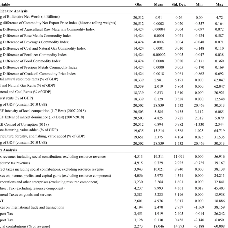
Data on billionaire net worth (in USD) are used to proxy for top incomes. The data are obtained from Forbes Magazine’s updated database of billionaires (2001 to 2018). Billionaires are identified based on their first name, last name, and their profile in Forbes magazine. Information from Wikipedia is used to fill in missing information on billionaire characteristics such as country of citizenship. The number of billionaires in the sample rose from approximate 565 in 2001 to 2,208 in 2018. Forbes Magazine’s billionaire database has been used in the literature to study wealth distribution (Piketty, 2014; Bagchi et al., 2016), the international mobility of billionaires (Sanandaji, 2014), the emergence of Russian billionaires (Treisman, 2016), and statistical regularities at the top end of the wealth distribution (Klass et al., 2006) among others. Summary statistics for the sample of analysis are provided in Table A1.

2.2 Commodity Windfalls

Data on commodity price shocks are obtained from the IMF (Gruss and Kebhaj, 2019). The commodity terms of trade index are based on international prices of up to 45 individual commodities, constituting broad categories of energy, metals, food and beverages, and agricultural raw materials. We calculate commodity price shocks by taking the first differences of the log of the price index as shown in equation (1) below.

(9)

Where 𝑃, is the natural log of the real price of commodity j in year t. Ω , , represents the commodity-and country-specific time-varying weights, which are based on three year rolling average trade flows over the previous three calendar years. Similar measures of commodity windfalls have been used by Arezki and Brückner (2012).7

In addition, variables on resource rents are also used to proxy for commodity windfalls. The data on natural resource rents come from the Changing Wealth of Nations dataset of the World Bank (2011) available from the World Bank’s World Development Indicators (WDI). Natural resource rents are defined as the difference between the unit price of resources and their unit cost of extraction, multiplied by the volume of resources extracted. Total natural resources rents are the sum of oil rents, natural gas rents, coal rents (hard and soft), mineral rents, and forest rents. The data have been widely utilized in the literature (Klomp and de Haan, 2016; Arezki and Gylfason, 2013). Summary statistics for the sample of analysis are provided in Table A1.

2.3 Tax data

Tax data are obtained from the UNU-WIDER ICTD government revenue dataset (Prichard et al, 2014). The dataset combines several sources of tax data compiled from IMF Article IV reports, thereby ensuring extensive coverage. These include IMF Government Finance Statistics (GFS), World Bank World Development Indicators (WDI), OECD Tax Statistics, OECD Revenue Statistics in Latin America dataset, CEPAL Tax Statistics, and the AEO African Fiscal Performance. The dataset includes a separate category for resource tax revenues, in addition to several other tax breakdowns. Data is available from 1980 to 2017. Summary statistics for the sample of analysis are provided in Table A1.

3. Estimation Strategy

In this section we present our empirical strategy.

To explore the effect of commodity price shocks on billionaire net worth we estimate the following equation:

𝐿𝑛𝐵𝐿𝑁𝑊_, 𝛼 𝛽 𝐷𝑓𝑙𝑛𝐶𝑜𝑚𝑃𝑟𝑖 _, 𝛾 𝐶𝑜𝑛𝑡𝑟𝑜𝑙𝑠 _, 𝜏 𝜐 𝜀_, (2)

Where 𝐿𝑛𝐵𝐿𝑁𝑊 is the log of billionaire net worth in USD for individual i at time t; 𝐷𝑓𝑙𝑛𝐶𝑜𝑚𝑃𝑟𝑖 is the log difference of the commodity price index in country c, 𝐶𝑜𝑛𝑡𝑟𝑜𝑙𝑠 is a vector of country-level controls including structure and size of the economy. 𝜏 is the year fixed effects and 𝜐 represents individual billionaire fixed effects. As a robustness check, we estimate equation (2) using country fixed effects instead of billionaire fixed effects. Alternatively, we also estimate equation (2) using resource rents in place of commodity price shocks.

7_{We employ a similar measure to calculate specific commodity sub‐indices. There are marginal differences in}

(10)

Our identification strategy allows us to account for several endogeneity issues. The commodity price shock variables are plausibly exogenous considering most countries are price takers in most commodities they trade hence limiting the simultaneity bias. We limit omitted variable bias in several ways. Billionaire fixed effects are used to account for time-invariant billionaire-specific and country-specific unobservable. This can include education, ability, as well as geographic location and main sector of activity if they do not vary over time. The year fixed effects capture common year shocks. We also include country-level covariates that capture the size and structure of the economy, that could be important predictors of billionaire net worth.

4. Top Income Results

In this section we present our main results.

5.1 Baseline

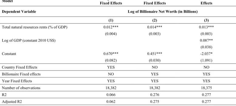
Table 1 presents our baseline estimates of the effect of commodity price shocks on billionaire net worth. Column 1 provides the estimates accounting for country and year fixed effects. This yields a positive effect of commodity price shocks (booms) on billionaire net worth, statistically significant at the 1% level. However, the estimates may be susceptible to omitted variable bias given several individual-specific time invariant characteristics including inherent ability and family background that may be important predictors of billionaire net worth. In column (2) we replace country fixed effects with billionaire fixed effects to account for these factors. The magnitude of the coefficient drops but the main results remain – positive commodity price shocks increase billionaire net worth, statistically significant at the 1% level. In column 3 we account for the size of the economy, which is positively correlated with billionaire net worth, suggesting scale effects where the net worth of billionaires increases with the size of the economy. Taking the estimates in column 3, a one percentage point increase in the log difference of commodity prices results in a 38% increase billionaire net worth. However, a percentage point increase in the growth rate of commodity prices is a sizeable increase. Thus a 1% increase in commodity prices translates to a 0.004 percent increase in billionaire net worth. A one standard deviation increase in the log difference of commodity prices leads to a 1.3% increase in billionaire net worth, which is roughly 1.5% of the sample mean of billionaire net worth. In table 2 we employ a measure of resource rents as an alternative to commodity price shocks. The results are consistent – resource rents are positively related to billionaire net worth, statistically significant at the 1% level irrespective of whether the specification includes country or billionaire fixed effects. The drawback of this measure is that it is unlikely to be exogenous.

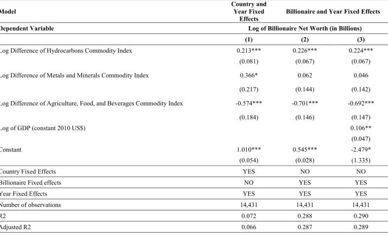
In table 3, we delve deeper into price sub-indices of specific groups of commodities. These commodity divisions include (i) hydrocarbons (crude, coal and natural gas) (ii) Metals and Minerals (base metals, precious metals, fertilizer) and (iii) Agriculture (raw materials), Food and Beverages. We find that hydrocarbons commodity price shocks (booms) are positively related with billionaire net worth, statistically significant at the 1% level, regardless of whether the specification includes country fixed effects (column 1) or billionaire fixed effects (columns 2 and 3). Positive agriculture, food, and beverage commodity price shocks are negatively related to billionaire net worth, statistically significant at the 1% level, regardless of

(11)

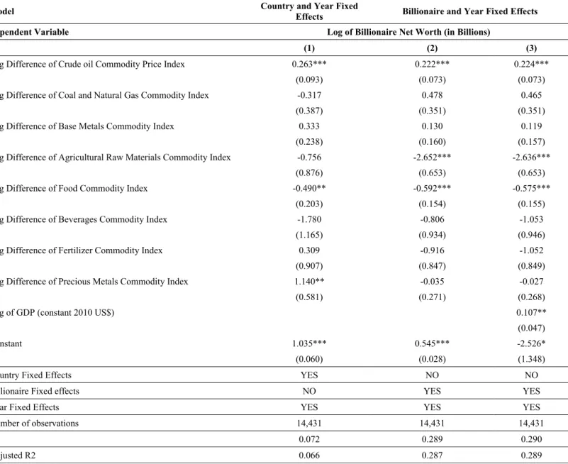
whether the specification includes country fixed effects (column 1) or billionaire fixed effects (columns 2 and 3). In table A2 in the appendix, we explore even more refined breakdowns of the commodity price index. We find that crude oil price shocks (booms) are positively related with billionaire net worth, while positive food price shocks are negatively related to billionaire net worth, both findings statistically significant at the 1% level.

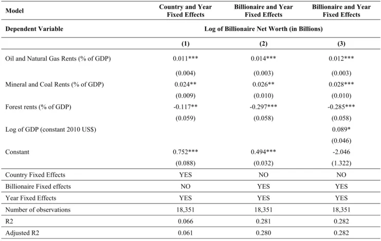
These results complement Isham et al. (2015) that finds countries with natural resources extracted for a narrow geographic region or economic base (point source natural resource) are predisposed to weakened institutional capacity. This may in turn limit the ability of governments to adequately tax top incomes. In contrast, economies with diffuse natural resources (livestock and agricultural produce) do not exhibit similar weak institutional capacity and have more robust growth recoveries. This is also consistent with the natural resource rents results as reported in table 4: billionaire net worth is positively correlated with point source natural resource rents such as oil and natural gas, mineral and coal rents, while negatively correlated with diffuse resources such as forest rents (statistically significant between 1 and 5%).

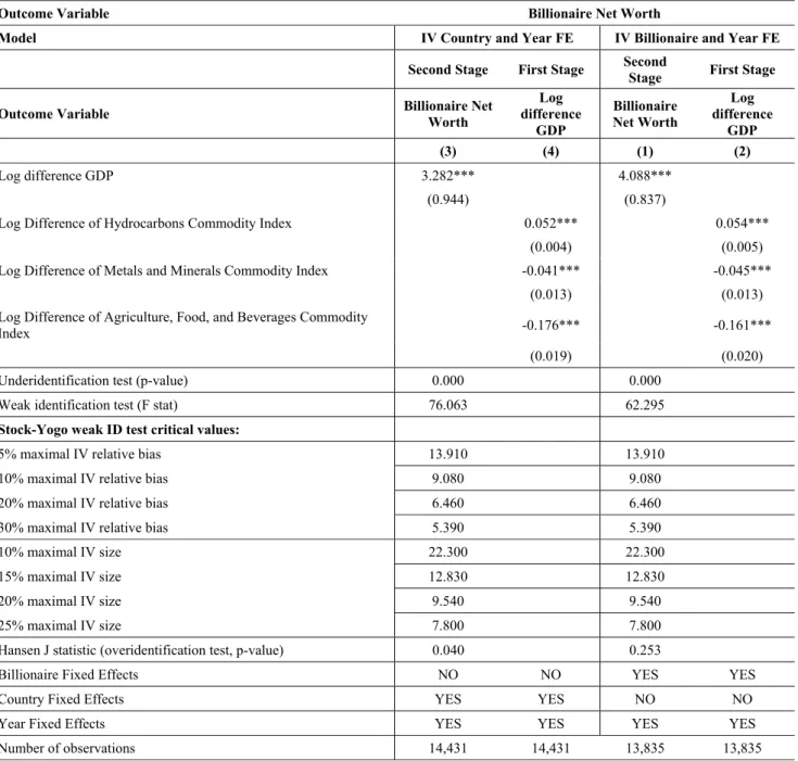
An alternative approach is to estimate the effect of economic growth on billionaire net worth using commodity price shocks as instruments. These findings are reported in table 5. Hydrocarbon commodity price shocks have a positive and statistically significant effect on economic growth, while price shocks from metals, minerals, agriculture, food and beverages have a negative and statistically significant effect on economic growth. Economic growth is positively related to billionaire net worth, with the coefficient being statistically significant at the 1% level. These findings stand whether billionaire or country fixed effects are employed. The instruments reject under-identification. The instruments also pass the over-identification test, especially when billionaire fixed effects are used, indicating that the validity of the instruments cannot be rejected. The instruments are also strong, given that they pass the weak identification test, exceeding the Stock and Yogo critical values.

The findings thus far point to a plausible mechanism whereby top income increase in the face of growth or commodity terms of trade shocks. We test whether this is conditional on the degree of market contestability/competition and quality of institutions in the economy. We use the sample average of the control of corruption quality of governance indicator. This captures perceptions of the extent to which public power is exercised for private gain, including both petty and grand. We also use the sample averages of the World Economic Forum’s indicators on the intensity of location and market domination. The former measure considers the distortive effect of taxes and subsidies on competition, the extent of market dominance, and competition in services. The market dominance indicator measures perceptions of whether corporate activity is characterized by a few business groups or many firms. For all indicators, higher values imply better governance/market contestability.

Table 6 reports the findings. All interactions between governance/competition and commodity price shocks have negative and statistically significant coefficients. The same results are found when the governance/competition variables are interacted with resource rents. The results indicate that in countries with more contestable markets and good governance, top incomes are less likely to increase as a result of positive commodity price shocks. These findings are consistent with Andersen et al., (2017) that finds that

(12)

exogenous shocks in petroleum income increase hidden wealth in offshore accounts for economies where institutional checks and balances are weak.8

5.2 Robustness Checks

Sector of activity and structure of the economy

The estimates provided thus far are based on parsimonious specifications. In the following, we explore the robustness of the baseline findings along several dimensions. First the structure of the economy may be an important predictor of billionaire net worth. Second the sector of billionaire activity may also matter, to the extent that it varies over time. In tables A3 and A4 we replicate tables 1 and 2 respectively with the inclusion of the share of manufacturing and Agriculture as a percent of GDP as additional covariates. The sign, significance and magnitude are relatively unchanged for the commodity price shock and resource rents coefficients.

The Forbes Magazine database does include data on the billionaire sector of activity that encompasses about 57 sectors of activity. However, this variable is measured with error given a single billionaire can be involved across multiple sectors. Furthermore, the 57 sectors do not seem to be mutually exclusive. We therefore recategorize the 57 sectors into 6 broad categories (see table A7) that include: (a) Agriculture (b) Extractives (c) Manufacturing (d) Services (e) IT and (f) Others. In tables A5 and A6 we present the results for commodity price shocks and resource rents respectively, after accounting for sector fixed effects for the narrow 57 categories, and the broad 6 categories. Our main results are robust. Indeed, the magnitude, sign and significance of the coefficients are similar to our baseline estimates.

Citizenship versus residency

Finally, our findings are based on the billionaire country of citizenship. The choice is logical given that a billionaire may exert greater influence in the country of her or his citizenship. However, this may not always be the case, and billionaires may have greater influence in their place of residence. Furthermore, there is some ambiguity in the case of dual citizenship, with the database in some cases assigning the citizenship at birth. In 2001, 1.2 percent of billionaires in the sample were not residents in their country of citizenship. This grew to 9.3 percent in 2018. Thus, we reproduce our baseline results using billionaire residency instead of citizenship in table A8. Our main results are robust.

5. Additional Results

In this section, we explore additional results related to tax policies and tax revenue mobilization following commodity price shocks.

(13)

Interaction with Taxes

We investigate whether higher taxes lessen the positive effect of commodity shocks and natural resource rents on billionaire net worth. Countries with greater capacity to tax may be able to capture some of the windfalls from commodity booms by extracting revenues from top incomes. As reported in table 7, we find no such effects. The coefficient of the interaction terms between tax revenues and commodity price shocks is statistically insignificant. This remains the case if we interact commodity price shocks with resource taxes, or the ratio of indirect over direct taxes. The results are similar when using resource rents, bar one exception. The interaction between total resource rents and the ratio of indirect over direct taxes is positive and statistically significant, albeit at the 10% level. The implication may be that a tax structure that favors indirect taxes allows billionaires to gather a larger share of commodity windfalls.

Effects of commodity price shocks on taxes and social contributions

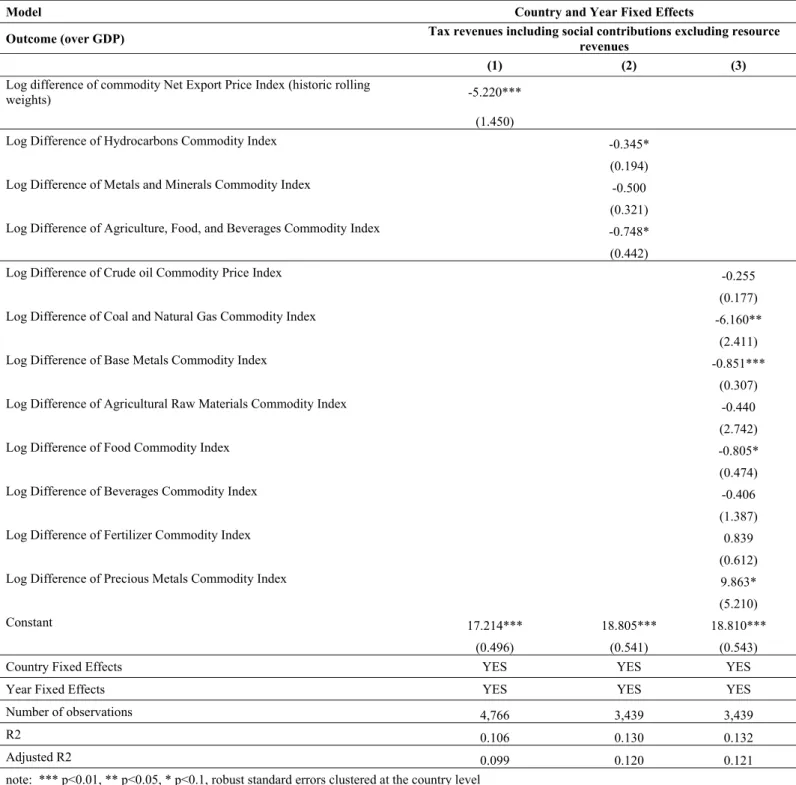
The inability of taxes to lessen the effects of commodity price shocks on top incomes, raises the question as to whether such shocks have direct effect on taxes themselves. In Table 8 we regress tax revenues as a percentage of GDP (excluding revenues from resources) on the log differences of the commodity price index. We uncover a negative coefficient for commodity price shocks, statistically significant at the 1 % level (column 1, table 7). These results are mirrored in table A9 using resource rents in place of commodity price shocks. Commodity price booms are associated with weakening non-resource tax capacity, which may explain why the effect of commodity price shocks on billionaire net worth are unaffected by the country's tax rates. Looking at subcomponents of the commodity price indices, hydrocarbons and agriculture, food and beverages have negative coefficients, statistically significant at the 10% level (column 2, table 8). Breaking down these sub-categories even further, base metals, coal and natural gas price shocks (commodity booms) have negative coefficients, statistically significant at least at the 10% level (column 3, table 8). The crude oil price shock variable has a negative effect but is statistically insignificant. The findings for the breakdown of resource rents are provided in column 2 of Table A9. Oil and natural gas rents are negatively related to tax revenues, the coefficient being statistically significant at the 1% level. This provides mixed evidence as to whether point source resource booms as opposed to diffused resource booms may weaken the tax capacity of economies.

We unpack these findings further by investigating the effects of commodity price shocks on the composition of tax revenues (as a share of GDP). As reported in table A10. The log difference of the commodity price index is negatively related to direct and indirect taxes, statistically significant at the 1% and 5% level respectively. There is a positive relationship with resource tax revenues, but the coefficient is not statistically significant. Table A11 replicates the findings of Table A10 using resource rents in place of commodity price shocks. Total resource rents are positively correlated with resource tax revenues, as expected, the coefficient being statistically significant at the 10% level. Resource rents are also negatively corrected with indirect taxes, with the coefficient being statistically significant at the 1% level. However, there is no statistically significant relationship with direct taxes. The evidence points to commodity price booms lowering non-resource tax revenues across the board, whether direct or indirect. However, the evidence is weaker with regards to resource rents and direct taxes.

(14)

An additional result we explore is whether commodity price shocks and resource rents have any effects on social contributions (as a % of total revenue). Results are presented in table A12. The coefficient for the log differences of commodity prices is negative and statistically significant at the 1% level (column 1, table A12). We find similar findings for natural resource rents - the coefficient is negative and statistically significant at the 1% level (column 3, Table A12). There are barely any statistically significant results for the sub-price indices with the exception of metals and minerals with a negative coefficient that is statistically significant at the 10% level (column 2, table A12). However, the findings are stronger when using with resource rates with coefficients for oil and natural gas rents as well as mineral and coal rents being negative and statistically significant at the 5% level. The results are suggestive that commodity price booms are negatively related to social contributions.

6. Conclusion

In this paper we explored the relationship between commodity booms and top incomes using billionaires net worth. Our main finding is that commodity booms increase billionaire net worth. We find that the type of resource matters – price shocks from point source resources such as hydrocarbons, where rents are more easily captured, are more likely to raise top incomes while price shocks from diffuse source resources are not. The positive relationship between commodity price shocks and top incomes is attenuated by a higher degree of competition in markets but is unaffected by taxes. In fact, we find that commodity price shocks tend to reduce the non-resource component of both direct and indirect taxes hence limiting scope for income transfers and redistribution. These findings contribute to the current policy debate on curbing the rise in top incomes that has been focused on wealth taxes as a possible instrument. While there is a strong rationale for a wealth tax especially following calamities its implementation can be challenging considering sophisticated tax avoidance for high net worth individuals. Our empirical finding highlighting the potency of competition policy is consistent with the primacy of ex ante interventions over ex post ones to address top income inequality.

(15)

References

Aghion P, Griffith R. (2005). Competition and Growth. Zeuthen Lectures, MIT Press.

Aghion, Philippe, Ufuk Akcigit, Antonin Bergeaud, Richard Blundell, and David Hemous (2019). “Innovation and Top Income Inequality.” Review of Economic Studies 86:1-45.

Alesina, Alberto and Roberto Perotti (1996). “Income Distribution, Political Instability, and Investment.”

European Economic Review. 40 (6), 1203–1228.

Alstadsæter, Annette, Niels Johannesen, Gabriel Zucman, 2018. “Who owns the wealth in tax havens? Macro evidence and implications for global inequality”, Journal of Public Economics, Volume 162, 2018, Pages 89-100.

Andersen, Jorgen Juel, Niels Johannesen, David Dreyer Lassen, and Elena Paltseva (2017). “Petro Rents, Political Institutions, and Hidden Wealth: Evidence from Offshore Bank Accounts.” Journal of the

European Economic Association 15(4): 818-860.

Arezki, Rabah and Markus Bruckner (2012). “Commodity Windfalls, Democracy and External Debt.”

The Economic Journal 122 (561): 848-866.

Arezki, Rabah and T. Gylfason (2013). “Resource Rents, Democracy, Corruption and Conflict: Evidence from Sub-Saharan Africa” Journal of African Economies 22(4): 552-569.

Arezki, R., Loungani P., van der Ploeg, R. and Venables T., (2014). Understanding International Commodity Price Fluctuations, Journal of International Money and Finance, Vol 42, April, pp. 1-8. Assouad, Lydia, Lucas Chancel, and Marc Morgan (2018). “Extreme Inequality: Evidence from Brazil, India, the Middle East, and South Africa.” American Economic Review, Papers and Proceedings 108:119-123.

Atkinson, Anthony B., Thomas Piketty and Emmanuel Saez (2011). “Top Incomes in the Long Run of history.” Journal of Economic Literature 49(1): 3-71.

Bagchi S., Svejnar J., Bischoff K. (2016). “Does Wealth Distribution and the Source of Wealth Matter for Economic Growth? Inherited v. Uninherited Billionaire Wealth and Billionaires’ Political Connections.” In: Basu K., Stiglitz J.E. (eds) Inequality and Growth: Patterns and Policy. International Economics Association. Palgrave Macmillan, London.

Banerjee, Abhijit and Thomas Piketty (2005). “Top Indian Incomes, 1922-2000.” World Bank Economic

Review 19(1):1-20.

Bartels, Larry M. (2008). Unequal Democracy: The Political Economy of the New Gilded Age. Princeton University Press.

Bivens, Josh and Lawrence Mishel (2013). “The Pay of Corporative Executives and Financial Professionals as Evidence of Rents in Top 1 Percent Incomes.” Journal of Economic Perspectives 27(3): 57-78.

Borge, Lars-Erik, Pernille Parmer, and Ragnar Torvik (2015). “Local Natural Resource Curse?” Journal of

(16)

Fleurbaey, M., & Peragine, V. (2013). Ex Ante Versus Ex Post Equality of Opportunity. Economica, 80(317), 118-130.

Freund, Caroline (2016). Rich People Poor Countries: The Rise of Emerging-market Tycoons and Their Mega Firms. Peterson Institute for International Economics, Washington DC.

Gruss, Bertrand and Suhaib Kebhaj (2019). “Commodity Terms of Trade: A New Database” IMF Working Paper WP/12/21.

Hsu, Shi-Ling (2014). The Rise and Rise of the One Percent: Considering Legal Causes of Inequality (November 5). FSU College of Law, Public Law Research Paper No. 698, FSU College of Law, Law, Business & Economics Paper No. 14-11.

Isham, Jonathan, Michael Woolcock, Lant Pritchett, and Gwen Busby (2005). “The Varieties of Resource Experience: Natural Resource Export Structure and the Political Economic of Economic Growth/” World

Bank Economic Review 19(2): 141-174.

Ing-haw Cheng and Wei Xiong (2014), The Financialization of Commodity Markets, Annual Review of

Financial Economics 6, 419-441.

James, Alexander, "US State Fiscal Policy and Natural Resources", American Economic Journal:

Economic Policy 7, 3 (2015), pp. 238-257.

James (2015) establishes a negative relationship between resource and non resource revenues as

the expression of a crowding out effect between these sources of revenue.

Klass, Oren S., Ofer Biham, Moshe Levy, Ofer Malcai, and Sorin Solomon (2006). “The Forbes 400 and Pareto Wealth Distribution.” Economic Letters 90: 290-295.

Klomp, Jeroen, and Jakob de Haan (2016). “Election Cycles in Natural Resource Rents: Empirical Evidence” Journal of Development Economics 121: 79-93.

Lansing, Kevin J., and Agnieszka Markiewicz (2016). “Top Incomes, Rising Inequality and Welfare.” The

Economic Journal 128: 262-297.

Leigh, Andrew, and Pierre van der Eng (2009). “Inequality in Indonesia: What Can We Learn From Top Incomes?” Journal of Public Economics 93: 209-212.

Lopez, Ramon E., and Eugenio Figueroa (2016). “Fundamental accrued capital gains and the Measurement of Top Incomes: An Application to Chile.” Journal of Income Inequality 14:379-394.

Ma, Lin and Dimitrije Ruzic (2020). “Globalization and Top Income Shares.” Journal of International

Economics 125, 2020.

Mehlum, Halvor, Karl Moene and Ragnar Torvik (2006). “Institutions and the Resource Curse,” The

Economic Journal 116:1-20.

Philippon, Thomas (2019). The Great Reversal: How America Gave Up on Free Markets. Harvard University Press.

(17)

Piketty, Thomas and Emmanuel Saez (2003). “Income Inequality in the United States, 1913-1998.”

Quarterly Journal of Economics 118(1):1-39.

Piketty, Thomas (2003). “Income Inequality in France, 1901-1998.” Journal of Political Economy 111(5): 1004-1042.

Piketty, Thomas (2014). Capital in the Twenty First Century. Cambridge MA: Harvard University Press. Prichard Wilson, Alex Cobham, Andrew Goodall (2014). The ICTD government revenue dataset. ICTD Working Paper 2014 19: 1–64.

Robinson, James A., Ragnar Torvik, and Thierry Verdier (2017). “The Political Economy of Public Income Volatility: With an Application to the Resource Curse.” Journal of Public Economic 145: 243-252. Rota-Graziosi, G., 2019, “The supermodularity of the tax competition game,” Journal of Mathematical Economics, 83, 25-35.

Ross, Michael (2001). “Does Oil Hinder Democracy?” World Politics 53(3):325–61.

Ross, Michael L. (2015). “What Have We Learned about the Resource Curse?” The Annual Review of

Political Science 18:239-259.

Sachs, Jeffrey D., and Andrew M. Warner (2001). “The Curse of Natural Resources.” European Economic

Review 45: 827-838.

Saez, Emmanuel, and Gabriel Zucman (2019). The triumph of injustice: How the rich dodge taxes and how

to make them pay. New York: Norton Co.

Sanandaji, Tino (2014). “The international mobility of billionaires” Small Business Economics 42:329-338.

Sokoloff, Kenneth L., and Stanley L. Engerman (2000). “Institutions, Factor Endowments, and Paths of Development in the New World.” Journal of Economic Perspectives 14(3): 217-232.

Treisman, Daniel (2016). “Russia’s Billionaires.” American Economic Review: Papers & Proceedings 106(5): 236–241.

World Bank, (2011). Changing Wealth of Nations. World Bank, Washington DC.

Wu, Tim (2018). The Curse of Bigness Antitrust in the New Gilded Age. Columbia University Press, New York.

(18)

Table 1: Price Shocks and Billionaire Net Worth

Model Country and Year _{Fixed Effects} Billionaire and Year _{Fixed Effects} Billionaire and Year _{Fixed Effects} Dependent Variable Log of Billionaire Net Worth (in Billions)

(1) (2) (3)

Log difference of commodity Net Export Price Index

(historic rolling weights) 0.622*** 0.387*** 0.380***

(0.187) (0.148) (0.146)

Log of GDP (constant 2010 US$) 0.145***

(0.053)

Constant 0.888*** 0.467*** -3.673**

(0.030) (0.030) (1.526)

Country Fixed Effects YES NO NO

Billionaire Fixed effects NO YES YES

Year Fixed Effects YES YES YES

Number of observations 20,512 20,512 20,502

R2 0.064 0.285 0.289

Adjusted R2 0.060 0.284 0.289

note: *** p<0.01, ** p<0.05, * p<0.1, Robust Standard Errors Clustered at the Billionaire level

Table 2: Natural Resource Rents and Billionaire Net Worth

Model Country and Year _{Fixed Effects} Billionaire and Year _{Fixed Effects} Billionaire and Year Fixed _Effects Dependent Variable Log of Billionaire Net Worth (in Billions)

(1) (2) (3)

Total natural resources rents (% of GDP) 0.012*** 0.014*** 0.013***

(0.004) (0.003) (0.003)

Log of GDP (constant 2010 US$) 0.087**

(0.038)

Constant 0.670*** 0.451*** -2.037*

(0.082) (0.030) (1.091)

R2 0.066 0.276 0.277

Adjusted R2 0.062 0.275 0.277

(19)

Table 3: Disaggregated Commodity Price Shocks and Billionaire Net Worth

Model Country and Year Fixed

Effects Billionaire and Year Fixed Effects Dependent Variable Log of Billionaire Net Worth (in Billions)

(1) (2) (3)

Log Difference of Hydrocarbons Commodity Index 0.213*** 0.226*** 0.224***

(0.081) (0.067) (0.067)

Log Difference of Metals and Minerals Commodity Index 0.366* 0.062 0.046

(0.217) (0.144) (0.142)

Log Difference of Agriculture, Food, and Beverages Commodity Index -0.574*** -0.701*** -0.692***

(0.184) (0.146) (0.147)

(0.047)

Constant 1.010*** 0.545*** -2.479*

(0.054) (0.028) (1.335)

R2 0.072 0.288 0.290

Adjusted R2 0.066 0.287 0.289

(20)

Table 4: Disaggregated Resource Rents and Billionaire Net Worth

(1) (2) (3)

Oil and Natural Gas Rents (% of GDP) 0.011*** 0.014*** 0.012***

(0.004) (0.003) (0.003)

Mineral and Coal Rents (% of GDP) 0.024** 0.026** 0.028***

(0.009) (0.010) (0.010)

Forest rents (% of GDP) -0.117** -0.297*** -0.285***

(0.059) (0.058) (0.058)

Log of GDP (constant 2010 US$) 0.089*

(0.046)

Constant 0.752*** 0.494*** -2.046

(0.088) (0.032) (1.322)

R2 0.066 0.281 0.282

Adjusted R2 0.061 0.280 0.282

(21)

Table 5: Economic Growth and Billionaire Net Worth using Disaggregate Price Shocks as Instruments

Outcome Variable Billionaire Net Worth

Model IV Country and Year FE IV Billionaire and Year FE Second Stage First Stage Second _Stage First Stage Outcome Variable Billionaire Net _Worth difference Log

GDP Billionaire Net Worth Log difference GDP (3) (4) (1) (2) Log difference GDP 3.282*** 4.088*** (0.944) (0.837)

Log Difference of Hydrocarbons Commodity Index 0.052*** 0.054***

(0.004) (0.005)

Log Difference of Metals and Minerals Commodity Index -0.041*** -0.045***

(0.013) (0.013)

Log Difference of Agriculture, Food, and Beverages Commodity

Index -0.176*** -0.161***

(0.019) (0.020)

Underidentification test (p-value) 0.000 0.000

Weak identification test (F stat) 76.063 62.295

Stock-Yogo weak ID test critical values:

5% maximal IV relative bias 13.910 13.910

10% maximal IV size 22.300 22.300

15% maximal IV size 12.830 12.830

20% maximal IV size 9.540 9.540

25% maximal IV size 7.800 7.800

Hansen J statistic (overidentification test, p-value) 0.040 0.253

Billionaire Fixed Effects NO NO YES YES

Country Fixed Effects YES YES NO NO

Year Fixed Effects YES YES YES YES

Number of observations 14,431 14,431 13,835 13,835

(22)

Table 6: Interaction with Institutions

Model Billionaire and Year Fixed Effects

Dependent Variable Log of Billionaire Net Worth (in Billions)

(1) (2) (3) (4) (5) (6)

Log Difference of Commodity Net Export Price Index x WEF

Local Competition (0717) -0.758**

(0.361)

Log Difference of Commodity Net Export Price Index x WEF

Market Dominance (0717) -0.488*

(0.253)

Log Difference of Commodity Net Export Price Index x WGI

Control of Corruption (0118) -0.326**

(0.153) Total natural resources rents x WEF Local Competition (0717) -0.018***

(0.005) Total natural resources rents x WEF Market Dominance

(0717) -0.023***

(0.005) Total natural resources rents x WGI Control of Corruption

(01-18) -0.009*

(0.005)

Log difference of commodity Net Export Price Index (historic

rolling weights) 4.224** 2.367** 0.387***

(1.855) (1.041) (0.144)

(0.028) (0.022) (0.003) Log of GDP (constant 2010 US$) 0.145*** 0.144*** 0.144*** 0.098** 0.104** 0.100**

(0.053) (0.053) (0.053) (0.049) (0.050) (0.048)

Constant -3.672** -3.663** -3.666** -2.333* -2.506* -2.401*

(1.525) (1.524) (1.523) (1.408) (1.430) (1.365)

Billionaire Fixed Effects YES YES YES YES YES YES

Year Fixed Effects YES YES YES YES YES YES

Number of observations 20,493 20,493 20,502 18,342 18,342 18,351

R2 0.290 0.290 0.290 0.280 0.282 0.278

Adjusted R2 0.289 0.289 0.289 0.279 0.281 0.278

(23)

Table 7: Commodity Price Shocks, Resource Rents and Tax Revenue Interactions

Dependent Variable Log of Billionaire Net Worth (in Billions)

(1) (2) (3) (4) (5) (6)

Log Difference of Commodity Net Export Price Index x Tax revenues (including social contributions and resource

taxes) (01-18) 0.016

(0.011) Log Difference of Commodity Net Export Price Index x

Resource Taxes over GDP (01-18) 0.018

(0.052) Log Difference of Commodity Net Export Price Index x

Indirect over Direct Taxes 0.030

(0.020) Total natural resources rents x Tax revenues (including

social contributions) (01-18) 0.0001

(0.000) Total natural resources rents x Resource Taxes over GDP

(01-18) 0.0005

(0.001) Total natural resources rents x Indirect over Direct Taxes

(01-18) 0.0003*

(0.000) Log difference of commodity Net Export Price Index

(historic rolling weights) 0.135 0.453*** 0.164

(0.206) (0.166) (0.174)

(0.003) (0.003) (0.003) Log of GDP (constant 2010 US$) 0.147*** 0.142*** 0.135** 0.099** 0.090* 0.104* (0.054) (0.053) (0.056) (0.048) (0.047) (0.060)

Constant -3.743** -3.601** -3.392** -2.363* -2.129 -2.481

(1.536) (1.528) (1.614) (1.375) (1.357) (1.713)

Billionaire Fixed Effects YES YES YES YES YES YES

Year Fixed Effects YES YES YES YES YES YES

Number of observations 20,426 19,980 19,183 18,281 17,899 17,152

R2 0.291 0.287 0.295 0.279 0.275 0.281

Adjusted R2 0.291 0.286 0.294 0.278 0.274 0.280

(24)

Table 8: Effect of Commodity Price Shocks on Tax Revenues

Model Country and Year Fixed Effects

Outcome (over GDP) Tax revenues including social contributions excluding resource _revenues

(1) (2) (3)

Log difference of commodity Net Export Price Index (historic rolling

weights) -5.220***

(1.450)

Log Difference of Hydrocarbons Commodity Index _-0.345*

(0.194)

Log Difference of Metals and Minerals Commodity Index _-0.500

(0.321) Log Difference of Agriculture, Food, and Beverages Commodity Index _-0.748* (0.442)

Log Difference of Crude oil Commodity Price Index _-0.255

(0.177)

Log Difference of Coal and Natural Gas Commodity Index _-6.160**

(2.411)

Log Difference of Base Metals Commodity Index _-0.851***

(0.307)

Log Difference of Agricultural Raw Materials Commodity Index _-0.440

(2.742)

Log Difference of Food Commodity Index _-0.805*

(0.474)

Log Difference of Beverages Commodity Index _-0.406

(1.387)

Log Difference of Fertilizer Commodity Index _0.839

(0.612)

Log Difference of Precious Metals Commodity Index _9.863*

(5.210)

Constant _17.214*** _18.805*** _18.810***

(0.496) (0.541) (0.543)

Country Fixed Effects YES YES YES

Number of observations _4,766 _3,439 _3,439

R2 _0.106 _0.130 _0.132

Adjusted R2 _0.099 _0.120 _0.121

(25)

APPENDIX

Table A1: Summary Statistics

Variable Obs Mean Std. Dev. Min Max

Billionaire Analysis

Log of Billionaire Net Worth (in Billions) _20,512 _0.91 _0.76 _0.00 _4.72

Log difference of Commodity Net Export Price Index (historic rolling weights) _20,512 _0.0002 _0.020 _-0.357 _0.164 Log Difference of Agricultural Raw Materials Commodity Index 14,424 0.00004 0.004 -0.097 0.072

Log Difference of Base Metals Commodity Index 14,424 -0.0001 0.021 -0.424 0.587

Log Difference of Beverages Commodity Index 14,424 -0.0002 0.004 -0.048 0.071

Log Difference of Coal and Natural Gas Commodity Index 14,424 0.0001 0.010 -0.148 0.110

Log Difference of Fertilizer Commodity Index 14,424 -0.00002 0.005 -0.047 0.038

Log Difference of Food Commodity Index 14,424 0.0008 0.020 -0.171 0.360

Log Difference of Precious Metals Commodity Index 14,424 0.0000 0.005 -0.170 0.169

Log Difference of Crude oil Commodity Price Index 14,424 0.0018 0.061 -0.862 0.692

Total natural resources rents (% of GDP) _18,339 _2.981 _6.193 _0.000 _62.047

Oil and Natural Gas Rents (% of GDP) _18,339 _2.019 _5.804 _0.000 _62.047

Mineral and Coal Rents (% of GDP) _18,339 _0.833 _1.610 _0.000 _20.921

Forest rents (% of GDP) _18,339 _0.129 _0.328 _0.000 _12.548

Log of GDP (constant 2010 US$) _20,502 _28.839 _1.532 _20.469 _30.513

WEF Intensity of local competition (1-7 Best) (2007-2018) _20,503 _5.585 _0.435 _3.112 _6.085 WEF Extent of market dominance (1-7 Best) (2007-2018) _20,503 _4.825 _0.725 _2.312 _5.879

WGI Control of Corruption (0118) 20,512 0.894 0.982 -1.330 2.344

Manufacturing, value added (% of GDP) _19,635 _15.214 _6.588 _1.025 _64.719

Agriculture, forestry, and fishing, value added (% of GDP) _19,651 _3.375 _4.104 _0.025 _31.535

Log of GDP (constant 2010 US$) _20,502 _28.839 _1.532 _20.469 _30.513

Tax Analysis

Tax revenues including social contributions excluding resource revenues 4,513 19.311 11.091 0.000 56.916

Resource tax revenues 4,915 0.729 2.925 -0.725 39.167

Direct taxes including social contributions, excluding resource revenue 3,943 10.021 8.740 0.000 38.138 Taxes on income, profits, and capital gains (excluding resource component) 4,056 5.973 4.341 0.000 24.211 Corporations and other enterprises (excluding resource component) 3,230 2.264 1.601 0.000 32.841

Indirect Tax (excluding resource component) 4,237 9.993 4.361 0.017 45.403

General Taxes on goods and services 3,381 5.283 3.196 0.000 18.938

VAT 2,601 4.976 3.017 0.000 18.886

Taxes on international trade and transactions 4,194 2.470 2.957 -1.569 38.159

Import Tax 3,451 1.919 2.405 -0.014 26.242

Export Tax 3,128 0.130 0.458 -2.140 6.050

(26)

Table A2: Disaggregated Commodity Price Shocks (8 categories) and Billionaire Net Worth

Model Country and Year Fixed _Effects Billionaire and Year Fixed Effects Dependent Variable Log of Billionaire Net Worth (in Billions)

(1) (2) (3)

Log Difference of Crude oil Commodity Price Index 0.263*** 0.222*** 0.224***

(0.093) (0.073) (0.073)

Log Difference of Coal and Natural Gas Commodity Index -0.317 0.478 0.465

(0.387) (0.351) (0.351)

Log Difference of Base Metals Commodity Index 0.333 0.130 0.119

(0.238) (0.160) (0.157)

Log Difference of Agricultural Raw Materials Commodity Index -0.756 -2.652*** -2.636***

(0.876) (0.653) (0.653)

Log Difference of Food Commodity Index -0.490** -0.592*** -0.575***

(0.203) (0.154) (0.155)

Log Difference of Beverages Commodity Index -1.780 -0.806 -1.053

(1.165) (0.934) (0.946)

Log Difference of Fertilizer Commodity Index 0.309 -0.916 -1.052

(0.907) (0.847) (0.849)

Log Difference of Precious Metals Commodity Index 1.140** -0.035 -0.027

(0.581) (0.271) (0.268)

(0.047)

Constant 1.035*** 0.545*** -2.526*

(0.060) (0.028) (1.348)

R2 0.072 0.289 0.290

Adjusted R2 0.066 0.287 0.289

(27)

Table A3: Commodity Price Shocks and Billionaire Net Worth with Control for Sectoral Composition of Economy

(1) (2) (3)

Log difference of commodity Net Export Price Index (historic

rolling weights) 0.637*** 0.319** 0.327**

(0.190) (0.146) (0.147)

Manufacturing, value added (% of GDP) 0.004 -0.017*** -0.020***

(0.007) (0.006) (0.006)

Agriculture, forestry, and fishing, value added (% of GDP) -0.014 -0.070*** -0.063***

(0.014) (0.012) (0.011)

(0.052)

Constant 1.046*** 1.027*** -2.589*

(0.140) (0.120) (1.466)

R2 0.065 0.287 0.289

Adjusted R2 0.060 0.286 0.288

(28)

Table A4: Natural Resource Rents and Billionaire Net Worth with Control for Economy Sectoral Composition

(1) (2) (3)

(0.004) (0.003) (0.003)

Manufacturing, value added (% of GDP) 0.003 -0.017*** -0.019***

(0.007) (0.006) (0.006)

Agriculture, forestry, and fishing, value added (% of GDP) -0.011 -0.069*** -0.065***

(0.015) (0.013) (0.012)

Log of GDP (constant 2010 US$) 0.081

(0.051)

Constant 0.745*** 1.000*** -1.279

(0.165) (0.117) (1.425)

R2 0.066 0.287 0.287

Adjusted R2 0.061 0.286 0.287

(29)

Table A5 Price Shocks and Sector Fixed Effects

Dependent Variable Log of Final Worth in Billions

(1) (2) (3) (4)

Log difference of commodity Net Export Price Index (historic rolling weights) 0.603*** 0.385*** 0.592*** 0.336** (0.188) (0.147) (0.201) (0.152)

6 Category Sector Fixed Effects (Others sector omitted)

IT 0.206*** -0.010 (0.078) (0.055) Agriculture -0.023 -0.250** (0.090) (0.109) Extractives 0.145*** -0.020 (0.054) (0.062) Manufacturing -0.009 -0.011 (0.040) (0.043) Services -0.0001 0.014 (0.034) (0.031)

57 Category Sector FE (Agriculture omitted omitted)

Apparel 0.030 0.160 (0.147) (0.144) Automotive 0.101 0.480*** (0.142) (0.138) Aviation -0.192 0.191 (0.183) (0.116) Banks 0.148 0.103 (0.193) (0.114) Beverages 0.089 0.158 (0.148) (0.212) Biotechnology 1.260*** 0.583*** (0.138) (0.176) Business 0.912* 0.588** (0.475) (0.269)

Casinos & Gaming 0.033 0.064

(0.233) (0.290)

Chemicals -0.092 0.474

(0.168) (0.321)

Coal -0.092 0.725***

(0.093) (0.137)

Construction & Engineering 0.007 0.183

(0.107) (0.158)

(30)

(0.212) (0.293) Consumer Services -0.245* 0.490*** (0.132) (0.160) Cruise Line 0.311*** -0.174 (0.089) (0.116) Diversified 0.208** 0.327*** (0.105) (0.126) Electronics -0.087 0.260 (0.231) (0.168) Energy 0.192* 0.323** (0.113) (0.138) Entertainment -0.722*** 0.385** (0.092) (0.157)

Fashion and Retail 0.217** 0.298**

(0.107) (0.125)

Finance -0.134 0.292**

(0.097) (0.122)

Finance and Investments 0.028 0.284**

(0.098) (0.120)

Food -0.087 0.247**

(0.136) (0.109)

Food and Beverage 0.105 0.257**

(0.105) (0.104)

Gambling & Casinos 0.250 0.211

(0.182) (0.202)

Gaming 0.219 0.192

(0.207) (0.230)

Healthcare -0.064 0.384**

(0.097) (0.183)

Hotels & Resorts -0.139 0.308

(0.256) (0.223) Information Technology -0.203 -0.106 (0.223) (0.334) Insurance -0.151 0.537*** (0.124) (0.167) Internet 0.088 -0.267 (0.183) (0.215) Internet Content-Entertainment -0.682*** (0.118) Investments 0.031 0.300** (0.106) (0.119) Leisure 0.104 0.428* (0.294) (0.232)

(31)

Logistics 0.008 0.518*** (0.128) (0.165) Luxury Goods 1.349*** 0.069 (0.302) (0.141) Manufacturing 0.025 0.267** (0.097) (0.119) Media 0.035 0.384*** (0.111) (0.130)

Media & Entertainment 0.199* 0.317**

(0.119) (0.132)

Medicine -0.251 0.356*

(0.216) (0.190)

Metals & Mining 0.402*** 0.247

(0.137) (0.193) Mineral -0.357*** (0.095) Oil -0.049 0.174 (0.105) (0.148) Pharmaceuticals 0.286* 0.380** (0.152) (0.179) Philanthropy/NGO 1.917*** 0.506*** (0.093) (0.132) Politics 0.724 0.401** (0.553) (0.184) Real Estate 0.082 0.261* (0.098) (0.154) Retail 0.204 0.321*** (0.124) (0.123) Semiconductors -0.185 0.237* (0.196) (0.136) Service -0.080 0.202* (0.105) (0.119) Shipping -0.167 0.341** (0.116) (0.163) Software 0.669** 0.216 (0.300) (0.153) Sports -0.240** 0.382*** (0.121) (0.139) Steel 0.376 0.266 (0.292) (0.291) Technology 0.237** 0.241* (0.117) (0.132) Telecommunications 0.346* 0.519***

(32)

(0.194) (0.201)

Transportation -0.460*** 0.543***

(0.119) (0.159)

Constant 0.906*** 0.468*** 0.961*** 0.203*

(0.041) (0.034) (0.099) (0.114)

Sector (6 Categories) Fixed Effects YES YES NO NO

Sector (57 Categories) Fixed Effects NO NO YES YES

Country Fixed Effects YES NO YES NO

Billionaire Fixed effects NO YES NO YES

R2 0.071 0.286 0.094 0.289

Adjusted R2 0.067 0.285 0.087 0.286

note: *** p<0.01, ** p<0.05, * p<0.1, Robust Standard Errors Clustered at the Billionaire level

Table A6 Resource Rents and Sector Fixed Effects

Dependent Variable Log of Final Worth in Billions

(1) (2) (3) (4)

Total natural resources rents (% of GDP) 0.012*** 0.014*** 0.011*** 0.013***

(0.004) (0.003) (0.004) (0.003)

6 Category Sector Fixed Effects (Others sector omitted)

IT 0.217*** -0.020 (0.083) (0.053) Agriculture -0.023 -0.245** (0.090) (0.101) Extractives 0.153*** 0.007 (0.054) (0.060) Manufacturing -0.003 -0.007 (0.041) (0.041) Services 0.008 0.015 (0.035) (0.030)

57 Category Sector Fixed Effects (Agriculture omitted omitted)

Apparel 0.041 0.166 (0.148) (0.136) Automotive 0.113 0.474*** (0.148) (0.127) Aviation -0.171 0.190* (0.183) (0.109) Banks 0.114 0.070 (0.203) (0.111)

(33)

Beverages 0.079 0.134 (0.148) (0.196) Biotechnology 1.269*** 0.581*** (0.144) (0.163) Business 0.922* 0.580** (0.476) (0.256)

Casinos & Gaming 0.044 0.062

(0.232) (0.284)

Chemicals -0.089 0.497

(0.166) (0.312)

Coal -0.131 0.733***

(0.095) (0.128)

Construction & Engineering 0.002 0.217

(0.107) (0.149) Consumer Products 1.085*** 0.523** (0.216) (0.258) Consumer Services -0.226* 0.490*** (0.133) (0.153) Cruise Line 0.331*** -0.153 (0.089) (0.110) Diversified 0.217** 0.325*** (0.107) (0.117) Electronics -0.081 0.255 (0.232) (0.156) Energy 0.204* 0.351*** (0.113) (0.129) Entertainment -0.702*** 0.360** (0.093) (0.159)

Fashion and Retail 0.232** 0.299**

(0.109) (0.117)

Finance -0.127 0.293***

(0.097) (0.113)

Finance and Investments 0.034 0.287***

(0.099) (0.111)

Food -0.078 0.235**

(0.137) (0.102)

Food and Beverage 0.100 0.244**

(0.106) (0.097)

Gambling & Casinos 0.243 0.199

(0.189) (0.196)

Gaming 0.231 0.233

(0.206) (0.232)

(34)

(0.099) (0.170)

Hotels & Resorts -0.138 0.323

(0.242) (0.226) Information Technology -0.183 -0.080 (0.224) (0.320) Insurance -0.140 0.541*** (0.124) (0.156) Internet 0.094 -0.224 (0.185) (0.203) Internet Content-Entertainment -0.664*** (0.122) Investments 0.043 0.300*** (0.106) (0.110) Leisure 0.118 0.412** (0.293) (0.206) Logistics 0.013 0.518*** (0.130) (0.156) Luxury Goods 1.373*** 0.120 (0.305) (0.133) Manufacturing 0.037 0.287*** (0.098) (0.110) Media 0.045 0.372*** (0.111) (0.122)

Media & Entertainment 0.213* 0.320***

(0.120) (0.123)

Medicine -0.242 0.370**

(0.215) (0.176)

Metals & Mining 0.427*** 0.299

(0.138) (0.187) Mineral -0.378*** (0.096) Oil -0.047 0.177 (0.105) (0.138) Pharmaceuticals 0.290* 0.400** (0.152) (0.167) Philanthropy/NGO 1.913*** 0.499*** (0.093) (0.123) Politics 0.713 0.405** (0.565) (0.192) Real Estate 0.083 0.264* (0.099) (0.145) Retail 0.211* 0.323*** (0.124) (0.115)

(35)

Semiconductors -0.164 0.264** (0.196) (0.127) Service -0.087 0.205* (0.106) (0.112) Shipping -0.163 0.338** (0.116) (0.156) Software 0.678** 0.232 (0.301) (0.143) Sports -0.262** 0.346*** (0.124) (0.130) Steel 0.354 0.274 (0.292) (0.285) Technology 0.241** 0.236* (0.120) (0.122) Telecommunications 0.359* 0.495*** (0.198) (0.186) Transportation -0.440*** 0.542*** (0.119) (0.151) Constant 0.690*** 0.449*** 0.767*** 0.185* (0.087) (0.034) (0.129) (0.106)

Sector (6 Categories) Fixed Effects YES YES NO NO

Sector (57 Categories) Fixed Effects NO NO YES YES

Country Fixed Effects YES NO YES NO

Billionaire Fixed effects NO YES NO YES

Year Fixed Effects YES YES YES YES

R2 0.074 0.277 0.098 0.279

Adjusted R2 0.069 0.276 0.090 0.276