Design and development of an airborne microwave radiometer for atmospheric sensing

Design and Development of an Airborne Microwave Radiometer

for Atmospheric Sensing

MASSACHUSES IN STIUTE

OF TECHNOLOGY

by

_{JUN 2}

1

2011

Michael P. Scarito

S.B. EECS, M.I.T. (2010)

LIBRARI ES

S.B. Physics, M.I.T. (2010)

Submitted to the Department of Electrical Engineering and Computer Science

in partial fulfillment of the requirements for the degree of

Master of Engineering in Electrical Engineering and Computer Science

at the

MASSACHUSETTS INSTITUTE OF TECHNOLOGY

ARWtNE

June 2011

@

Massachusetts Institute of Technology 2011. All rights reserved.

A u th or ...

...

Department of Electrical Engineering and Computer Science

May 20, 2011

Certified by... s ... ...

William

J.

Blackwell

Senior , MIT Lincoln abo tory

visp!-C ertified by ...

...

LKid

H. Staelin

Professor of Electrical Engineering

Thesis Supervisor

Accepted by ...

kChristopher

J.

Terman

Chairman, Department Committee on Graduate Theses

This work is sponsored by the National Oceanic and Atmospheric

Administra-tion under Air Force Contract #FA8721-05-C-0002. Opinions, interpretaAdministra-tions,

con-clusions, and recommendations are those of the author and are not necessarily

endorsed by the United States Government.

Design and Development of an Airborne Microwave Radiometer for

Atmospheric Sensing

by

Michael P. Scarito

Submitted to the Department of Electrical Engineering and Computer Science on May 20, 2011, in partial fulfillment of the

requirements for the degree of

Master of Engineering in Electrical Engineering and Computer Science

Abstract

Satellite-based passive microwave remote sensing is a valuable tool for global weather monitoring and prediction. This thesis presents the design and development of a low-cost airborne weather sensing instrument to independently validate a satellite-based sen-sor platform. The NPOESS Aircraft Sounder Testbed - K-band (NAST-K) is a passive microwave radiometer operating over approximately 200 MHz bandwidth centered at 23.8 GHz and 31.4 GHz, whose data can be used to find surface water, humidity, and temperature conditions. NAST-K flies along with the existing NAST-M instrument at an altitude of 18 km in the NASA ER-2 high altitude aircraft. The primary function of NAST-K is to provide coverage of channels 1 and 2 of the Advanced Technology Microwave Sounder (ATMS) aboard the NPOESS Preparatory Project (NPP) satellite, scheduled to be launched in October 2011. The combined NAST-M/K system can validate the per-formance of ATMS on all channels with data products up to 17km, by underflying the satellite along the same ground track and collecting correlated data. NAST-K has full-width at half maximum beamfull-widths of 7.4' and 6.80 for the two channels respectively, which is approximately consistent with NAST-M. The effective spot size of NAST-K is 2.3km in diameter for the wider 23.8GHz channel at nadir, providing an areal resolu-tion approximately 1000 times greater than ATMS. The major contriburesolu-tions of this thesis include the system-level design of NAST-K, the development of the video amplifier and embedded environmental monitor, and the analysis of the antenna system.

Thesis Supervisor: William

J.

Blackwell Title: Senior Staff, MIT Lincoln Laboratory Thesis Supervisor: David H. Staelin Title: Professor of Electrical Engineering

Acknowledgments

I would like to thank Bill Blackwell for his guidance throughout the development of this

project. Bill made himself very accessible despite his busy schedule, and he provided important encouragement to help me push forward in the project. In addition, I want to recognize Vince Leslie for serving as an informal second mentor on this project. Together, they were both tremendously useful in providing a weather science perspective for the work, as well as important lessons learned in the development of an airborne instrument from their past work on NAST-M.

Prof. Dave Staelin was an excellent technical resource. His extensive knowledge about practical radiometer design was very informative when determining project re-quirements. Prof. Jose Martinez of Northeastern University helped substantially with the initial antenna design and provided significant guidance as I made refinements to the design later on.

I worked with many staff members at M.I.T. Lincoln Laboratory to develop this

project, and they were all very helpful. Idahosa Osaretin, Mike DiLiberto, Dave Kusinsky, and Joe Costa all contributed advice on the system design. Allan Nichols, Larry Rether-ford and Bob Bucknam provided a lot of support on the mechanical side. They took my rough models and produced designs that we could actually build. Larry helped in a big way by taking measurements of the actual aircraft in Edwards, CA, since our drawings were incomplete. One person who really went out of his way to help was Jeff Shultz. On several occasions he took time out of his schedule to go over my circuit designs with me and point out any potential issues, even though NAST-K was not his project.

Contents

1 Introduction 15 2 Background 2.1 Microwave Radiometry. ... 2.1.1 Antenna Gain ... 2.1.2 Receiver gain ...

2.1.3 Noise equivalent delta-temperature . . . .

2.2 Radiative Transfer ...

2.2.1 Atmospheric Absorption . . . . 2.2.2 Brightness Temperature . . . .

2.3 Atmospheric Science in K- and Ka-bands . . . . .

2.4 Receiver Calibration . . . . 2.4.1 Ground Calibration . . . . 2.4.2 Operational Calibration . . . . 2.5 Antenna physics ... 2.5.1 Parabolic reflectors . . . . 2.5.2 Horn antennas . . . .

2.5.3 Matching the horn pattern to the reflector

2.6 NAST-M ... ... 3 Aircraft Sensor Design and Development

3.1 Overview . . . . 3.2 Antenna assembly . . . .

3.3 Radiometer front-end (RFE) . . . . 3.4 Video amplifier . . . . 19 . . . . 19 . . . . 19 . . . . 20 . . . . 2 1 . . . . 22 . . . . 23 . . . . 24 . . . . 25 . . . . 25 . . . . 26 . . . . 26 . . . . 27 . . . . 27 . . . . 29 . . . . 31 . . . . 3 1 33 . . . . 34 . . . . 34 . . . . 36 . . . . 37

3.5 System power and grounding . . 3.5.1 Power Conditioning Unit

3.5.2 Grounding ... 3.5.3 EM I . . . . 3.6 Flight computer ... 3.6.1 Hardware ... 3.6.2 Operating System ... 3.6.3 Instrument Software . . . . 3.7 Digital electronics . . . . 3.7.1 Camera . . . . 3.7.2 Ethernet . . . .

3.7.3 Embedded Environmental Monitor .

3.8 Electrical integration . . . . 3.8.1 NAST-M . . . . 3.8.2 Aircraft Experimenter Interface Panel

3.9 Mechanical integration . . . .

3.9.1 Flight computer housing . . . .

3.9.2 RFE housing . . . . 3.9.3 Scan assembly . . . . 3.9.4 Aircraft integration . . . . 3.10 Concept of operations . . . . 4 Antenna Subsystem 4.1 D esign . . . . 4.1.1 Feed . . . . 4.1.2 Reflector . . . . 4.1.3 Geometry . . . . 4.2 Analysis . . . . 4.2.1 Conventions . . . . 4.2.2 Horn antenna . . . . 4.2.3 Horn and reflector system . . . . 4.3 Performance . . . . . . . . 38 . . . . . . . . . 38 .. ... 38 ... ... 39 ... ... 39 . . . . 40 . . . .- 41 . . . . 42 . . . . 43 . . . . 43 . . . . 44 . . . . 44 . . . . 44 . . . .- - - . . 44 . . . . 45 . . . . 45 . . . . 46 . . . . 46 . . . . 48 . . . . 49 . . . . 50 55 . . . . 56 . . . . 56 . . . . 57 . . . . 59 . . . . 59 . . . . 59 . . . . 59 . . . . 60 . . . . 61

4.3.1 4.3.2 4.3.3 4.3.4 Beam shape .... Beam efficiency . . Projected spot size Polarization . . . .

5 Embedded Environmental Monitor 5.1 Hardware ...

5.2 Software ... 6 Conclusions

6.1 System design . . . .

6.2 Antenna system ...

6.3 Embedded environmental monitor ... 6.4 Future work ... ... 6.5 Conclusions ... ... A Antenna Polarization Patterns

B PCB Schematics and Layouts

References 81 81 81 82 83 83 85 95 103 . . . . . . . . . . . . . . . . . . . . . . . .

List of Figures

2-1 Atmospheric transmittance in the microwave band . . .

2-2 Cross-section geometry of an offset parabolic reflector .

2-3 Cross-section geometry of a conical horn antenna . . . . 3-1 3-2 3-3 3-4 3-5 3-6 3-7 3-8 3-9 3-10 4-1 4-2 4-3 4-4 4-5 4-6

NAST-K block diagram . . . .

Radiometer Front-end Block Diagram ...

NAST-K power connections . . . .

Flight computer enclosure I/O panel ...

NASA ER-2 aircraft, isometric drawing . . . .

Radiometer front-end enclosure, top view ... Radiometer front-end enclosure, angled view ...

NASA ER-2 wing pod ...

NAST-M/K in ER-2 wing pod, side view ...

NAST-M/K in ER-2 wing pod, detail view ....

Profile drawing of parabolic reflector ...

Model of parabolic reflector ...

Geometric conventions for reflector system . ...

Antenna gain for the reflector configurations . . .

Geometry to find projected spot size on the earth Elliptical polarization conventions . . . .

A-1 Major axis polarization angle versus look angle - K-band

A-2 Major axis polarization angle versus look angle - K-band

flat plate reflector parabolic reflector

A-3 Major axis polarization angle versus look angle - Ka-band flat plate reflector A-4 Major axis polarization angle versus look angle - Ka-band parabolic reflector

. . . . 35 . . . . 36 . . . . 39 . . . . 40 . . . . 46 . . . . 47 . . . . 47 . . . . 49 . . . . 50 . . . . 51

Elliptical eccentricity versus look angle -K-band flat plate reflector . . Elliptical eccentricity versus look angle -K-band parabolic reflector. Elliptical eccentricity versus look angle -Ka-band flat plate reflector Elliptical eccentricity versus look angle -Ka-band parabolic reflector

A-5 A-6 A-7 A-8 B-1 B-2 B-3 B-4 B-5 B-6

Video amplifier schematic . . . . Video amplifier PCB layout . . . . Embedded environmental monitor schematic (1/3) ...

Embedded environmental monitor schematic (2/3) ... Embedded environmental monitor schematic (3/3) ...

Embedded environmental monitor PCB layout ...

. . . 90 . . . 91 . . . 92 . . . 93 . . . . 96 . . . . 97 . . . . 98 . . . . 99 . . . . 100 . . . . 101

List of Tables

3.1 _{Radiometer front-end performance specification . . . . 36} 3.2 Receiver noise equivalent delta-temperature (ATrms) on NAST-K and ATMS 37

4.1 Beamwidth for flat plate and parabolic reflectors ... 64 4.2 Beam efficiency for the flat plate and parabolic reflectors . . . . 66

4.3 Boresight distance comparison between NAST-M/K and ATMS over look an gle . . . 69 4.4 Spot size comparison between NAST-K, NAST-M, and ATMS . . . . 69

Chapter 1

Introduction

Satellite-based remote sensing is one of the primary data sources for atmospheric weather measurement, modelling, and forecasting. Compared with the alternative of direct ob-servation tools such as ground stations, weather balloons, or rocketsondes, which only provide localized points of data, remote sensing provides global coverage at high reso-lution updated multiple times daily The tradeoff is that instead of directly measuring parameters such as temperature, barometric pressure, humidity, and wind speed and direction, these parameters must be inferred by the manner in which the atmosphere ab-sorbs, transmits, or reflects electromagnetic radiation in the microwave, infrared, visible, and ultraviolet regions.

The current operational weather satellite system of the National Oceanic and Atmo-spheric Administration (NOAA) is the Polar Operational Environmental Satellite (POES) system. This system provides global coverage four times per day, and includes several passive remote sensing instruments for weather observation. The POES payloads include two microwave sounders: the Advanced Microwave Sounding Unit (AMSU), and addi-tionally the Microwave Humidity Sounder (MHS) on newer satellites. These instruments are primarily intended to measure atmospheric humidity with respect to altitude, as well as water content in clouds[15]. Microwave sensors have lower spatial resolution than their infrared or visible counterparts, but they have the distinct advantage of being able to operate through cloud obscuration, which is likely when the weather data is the most valuable. The next generation platform for NOAA is the National Polar-orbiting Oper-ational Environmental Satellite System (NPOESS). The first satellite in this system, the

NPOESS Preparatory Project (NPP), is currently scheduled to be launched in October

2011. The satellite will contain a new microwave radiometer, the Advanced Technology Microwave Sounder (ATMS), which is the next generation replacement for AMSU-A.

The primary work pertaining to this thesis, the NPOESS Atmospheric Sounder Testbed

-K-band (NAST-K), is a new passive microwave radiometer design measuring two chan-nels near 23.8 GHz (K-band) and 31.4 GHz (Ka-band). These chanchan-nels are primarily used together to estimate cloud liquid water, integrated water vapor, and surface temperature. Radiance observations in the K-band region are more strongly attenuated due to water vapor than those in the Ka-band, and the relatively unattenuated K-band signal can be fit with the expected emissivity of the Earth's surface at its surface temperature [18]. The principal function of NAST-K is to validate the two corresponding channels on ATMS. When flown along with the heritage instrument NAST-M, the pair provides coverage of most of the channels on ATMS with independently designed receivers. In the mission plan, NAST-M and NAST-K will fly on a high-altitude aircraft directly below the ground track of the satellite. When the satellite passes overhead, the two airborne instruments will be collecting data which is both temporally and geographically coincident with the satellite data. As NAST-M/K can be extensively calibrated before and after the satellite under-flight, the two data sets can be compared against each other in order to demon-strate proper performance of ATMS.

The original plan called for NAST-K to be an upgrade of the NAST-M instrument, but the decision was soon made to create NAST-K as a separate instrument due the lack of space to add hardware to the NAST-M payload. This provides the advantage of having two separate independently-operating instruments available, where the failure of one will not affect the other, and where the two instruments can be deployed individually.

NAST-K operates as a cross-track scanner, collecting data in a swath to the left and

right of the aircraft as it flies forward. This design is consistent with that of NAST-M, which will allow NAST-M and NAST-K to operate in a synchronized configuration.

NAST-M and NAST-K have very similar antenna beamwidths which will allow them to

collect easily correlated data from the same paths through the atmosphere. NAST-K does provide several changes over the NAST-M design which are optimized for the lower fre-quency of operation. These include a direct-detect radiometer front end which provides a reduced noise figure over a superheterodyne design at the cost of more challenging RF

bandpass filters, a single radiometer feed for both frequency bands, an offset parabolic reflector to provide a tighter pencil-beam, and new voltage and temperature monitoring instrumentation.

NAST-K will be initially deployed along side NAST-M in the NASA ER-2 high altitude

aircraft. Both NAST-M and NAST-K are mounted in the rear of the ER-2 wing pod, with support electronics in the middle of the pod. NAST-K views the earth through a hole cut in the bottom of the pod, allowing the instrument to look from side to side. The pod will have an additional hole cut in the top allowing the instrument to look up into space as a calibration reference. NAST-M has demonstrated the validity of airborne measurement for satellite microwave radiometer calibration through its performance on several flight campaigns. The addition of NAST-K will expand its capability to provide temperature and humidity sensing from the surface up through an altitude of 17 km.

I have supported the design of most aspects of the NAST-K system. I have

pro-duced two original printed circuit board designs: the video amplifier which amplifies and buffers the output of the radiometer front end in order to pass it to the analog-to-digital converter, and the embedded environmental monitor which measures temperatures and supply voltages across the system, particularly around the radiometer front end. I have designed a parabolic horn and reflector model to evaluate the performance of the de-sign, and designed a preliminary parabolic reflector for manufacturability. Furthermore,

I have developed an initial parabolic reflector solid model for manufacturability. For the

radiometer system, I determined the required performance parameters to provide com-patibility with ATMS. I specified and sourced many of the parts in the system, including the scan drive motor, the flight computer system and enclosure, and the camera system and support electronics. I set up the initial software platform for development on the

NAST-K flight computer, and set up the hardware peripherals on the flight computer.

For the embedded environmental monitor, which was intended to be shared between

NAST-K and the MicroMAS project, I worked with the MicroMAS team to determine

Chapter 2

Background

2.1

Microwave Radiometry

Microwave radiometry is simply the passive measurement of power incident on an an-tenna at a given frequency. In remote sensing applications, the anan-tenna is typically highly directional, receiving energy from a localized area. The physical parameter being mea-sured is the thermal radiation from the earth or from space and how much this radiation is reflected or absorbed by the Earth's surface or by matter in the atmosphere. Since we are intending to measure thermal energy, the received power levels are extremely low. For some perspective, when discussing a normal radio receiver a typical figure of merit is the signal-to-noise ratio. In our case, the parameter of interest is exactly that thermal noise, which we must sense with enough power to detect minute changes. To make mat-ters worse, unlike a traditional receiver we cannot do anything to correlate our signal and increase the effective signal-to-noise ratio, since we are measuring a random process. This means that any noise introduced anywhere in the receiver system will decrease the effective sensitivity of the system, because it will impose a lower limit on the change in power that we can detect in any finite time interval [7].

2.1.1

Antenna Gain

When our radiometer is observing an environment, it does so through the use of an an-tenna. This antenna has a variable gain with respect to both frequency and look angle

like our antenna gain to be flat across this region. It should be noted that in some cases a variable antenna gain over frequency can be calibrated for, but it can present certain issues as we will see in Section 2.4.2. Antennas are passive elements, meaning the in-tegral of the gain per solid angle over the entire far field sphere around the antenna is equal to that of an isotropic antenna, minus any losses. Thus, when an antenna has gain above unity in one region, it has corresponding gain below unity in other regions. For a microwave radiometer, this is an interesting result, because neglecting losses in the an-tenna, a received power level will correspond to a specific average incident power density (power per solid angle) weighted over the antenna beam, and this power density to re-ceived power relationship is independent of the specifics of the antenna used. As the beam pattern of the antenna changes, only the weighting for the average will change, so if lossless antennas with different beam patterns are viewing different-sized scenes with the same power density, their power output will be identical to each other [25].

2.1.2 Receiver gain

Measurements made by a microwave radiometer are sampled as an analog voltage, which

is a rectified and low-pass filtered measurement of the signal within the RF pass-band of the system. This voltage is proportional to the received power. If we denote the power per unit frequency exiting the feed port of the antenna <a (v, t) and the gain of the receiver

Gr (v), then the signal level at the detector will be Dd (v, t) = 0a(v, t) Gr (v). The detector

has a response proportional to its input power. If we denote the detector response as

Gd(v), and assume some additional gain Go for the system following rectification (which does not have a frequency dependence because it comes after rectification), we have the instantaneous output voltage

V,(t) GO Gd(v)Gr (v) )a(v,t) dv. (2.1)

This voltage is typically low-pass filtered, so as to appear as V, (t) convolved with the tail of an exponential function with unity area. To simplify this model, we assume that the receiver gain is zero outside of some passband, and further that the response of the detector is flat within that passband. If our receiver is centered at some v = ve with

passband width Av, the output voltage is then

vc+Av/2

Vo(t) = Gvj GdGr (V)<(Da(V, t) dv. (2.2)

Since we are eventually interested in finding an average power level Pa in the passband, rather than a power per unit frequency, we can simplify the model further to assume a power level and receiver response that do not vary with frequency. In this case we assume that Pa ~1 <D(v)Av. This then simplifies the signal to

Vo(t) = GvGdGr Pa (t). (2.3)

We can then solve for the input power required to produce a given output voltage as

Pa(t ) = V(t) (2.4)

GdGrGv

In practice, the constant of proportionality is found through the periodic calibration pro-cess (see Section 2.4.2) so we are primarily concerned with the linear relationship between

Pa and V. Since the white calibration signals pass through the receiver and detector, as

long as we assume a white signal over the pass band from the measured signal, the as-sumptions made about the receiver and detector gain response over frequency are actually unnecessary.

2.1.3

Noise equivalent delta-temperature

A performance parameter for microwave radiometer sensitivity is the root-mean-square

(RMS) noise equivalent delta-temperature, or ATrms. This figure gives the error associated with a given brightness temperature measurement. The noise equivalent temperature is based on the integration time, the receiver bandwidth, and the noise temperatures of the receiver and the environment. First, the receiver temperature is found as

where NF is the receiver noise figure and Ta is the ambient noise temperature. The noise equivalent delta-temperature is then

Ta±+Tr

ATrms = Tr (2.6)

where T is the integration time and Av is the bandwidth [25].

2.2

Radiative Transfer

A radiometer designed for weather sensing is intended to receive radiation incident on

the Earth from space, or radiating from the Earth's surface or the atmosphere. Before this radiation reaches the radiometer antenna and can be measured it can be absorbed or reflected by the Earth's surface or by matter in the atmosphere. If we are searching for something that is primarily radiative at a certain frequency, then a higher signal indicates more of that thing. On the other hand, if we are searching for something that attenuates at a certain frequency, we are looking for a lower signal. We typically require some sort of baseline, so an example measurement might compare signals at two frequencies: one which is strongly attenuated by the matter of interest, and another which is negligibly attenuated. Finally, we may be interested in something which is reflective at a certain frequency, in which case a higher signal would indicate a weaker feature for an airborne or satellite-borne sensor, whereas a higher signal would indicate a stronger feature for a ground-based sensor.

It is important to remember that in interpreting data from any remote sensing system, we must determine not only the value and distribution of some physical parameter but also the very nature of the scene being viewed. There are multiple phenomena which could produce the same response in a given measurement. As an example, when viewing the surface over the earth, over land we would view much more intense radiation in the microwave band than over water. This is due to the fact that water is highly reflective at microwave frequencies compared to land, and the radiation being reflected is primarily incident from the cosmic microwave background of outer space. The reduced signal could also be due to strong attenuation of radiation from land by clouds. To interpret any measurement of a remote sensing system, the data is frequently combined with a

host of different measurements in order to disambiguate the complicated interactions in

atmospheric physics.

2.2.1 Atmospheric Absorption

0.9 0.8 -0.7 - -0.5I- \ -C r -I f 0.4 - -0.6 0.5 -H 0.4-I 0.3-1 0.2-0.1 I 0_{0 50 100 150 200 250} Frequency (GHz)

Figure 2-1: Atmospheric transmittance in the microwave band, based on the 1976

Stan-dard Atmosphere[17]. The transmittance corresponds to viewing a non-reflective surface

from space looking at nadir. The solid green line is the transmittance with no

atmo-spheric water vapor, and the dashed blue line is the transmittance with water vapor from

the 1976 standard included. Several relevant frequency bands for oxygen and water

va-por sensing are shown. The data is generated using the radiative transfer software from

Rosenkranz[20].

Any radiation sensed by a high altitude radiometer will be measuring a combination

of the radiated energy from the atmosphere and the radiated energy from the Earth's

surface. Depending on the altitude at which the energy is radiated, the energy will be

attenuated by the atmosphere by a varying magnitude. A typical transmittance for

en-ergy radiated by the Earth's surface is shown in Figure 2-1. This plot shows the strong water vapor absorption bands at 23.8 GHz and 183 GHz, and gives an idea of how the two channels at 23.8 GHz and 31.4 GHz can be compared to determine atmospheric wa-ter content. These absorption bands behave differently depending on pressure, where at a lower pressure an absorption band will be narrower and at a higher pressure the absorption band will broaden. This allows a radiometer with a series of channels spaced out around the center of an absorption band to measure phenomena at varying altitudes. This technique is described in [2] and is the reason why many radiometers have a bank of double-sideband channels centered about some frequency.

2.2.2

Brightness Temperature

Rather than antenna power, most atmospheric science models will use the equivalent brightness temperature when interpreting data from microwave radiometers. Brightness temperature, or Tb, is the temperature of a black body which would produce the same power as a given measurement. A black body is an idealized physical object which absorbs all incident radiation and radiates entirely incandescently. The intensity of this incandescent radiation is described by Planck's law. We can use Planck's law to find the time-averaged power density per unit frequency, per unit solid angle, at a given frequency, for a black body at a given temperature by the relationship

Bv (T) = 2 e1 (2.7)

c ekr _

where h ~ 6.626 x 10-34 m2 kg s-1 is Planck's constant and k ~ 1.381 x 10- 23 m2 kg s-2K-1

is the Boltzmann constant. This appears to be a very nonlinear relationship with temper-ature, but we can make a simplification. Since our frequency is very low compared to temperature, or more specifically hv

<

kT by two orders of magnitude at T = 300 K and

v = 31.4 GHz, we can instead use the simpler Rayleigh-Jeans law, which gives us 2v2k

Bv(T) c2 T, (2.8)

or rewriting for temperature,

[25] Since we have no information about how the power varies over our passband, only

a total power, we must simplify the law by assuming a constant TB(v)/Bv across the passband. This allows us to define Pa in terms of a single By as

Pa = v,s/ 2

B(v)

dv ~

By

Av. (2.10)

Jv,-Av'/2

This holds so long as Av < v. The modified Rayleigh-Jeans relationship is now

TB(V) (

2v

k

Pa. (2.11)

This is a convenient linear relationship between received power and brightness tempera-ture.

2.3 Atmospheric Science in K- and Ka-bands

The 23.8 GHz and 31.4 GHz channels in AMSU, ATMS, and NAST-K are commonly used to measure surface brightness temperatures and atmospheric water content. There are several algorithms provided by NESDIS for retrieving physical parameters from bright-ness temperatures recorded at these frequencies [18]. For data collected over the ocean, these two channels can be used to calculate cloud liquid water and water vapor in the ver-tical column viewed by the instrument. On land, snow cover can be characterized using the brightness temperature difference between the two channels. Snow water equivalent, which is a parameter describing the equivalent depth of pure water in a region of snow cover, can be estimated as well. Using one of the channels from NAST-M, at 50.3 GHz, in conjunction with the two NAST-K channels we can find sea ice concentration as a percentage of the surface area covered by the measurement spot. We can also estimate land surface temperature and surface emissivity at these three frequencies using their brightness temperatures [18].

2.4 Receiver Calibration

Calibration is an important part of any instrumentation system. In the case of a mi-crowave radiometer, gain calibration is critical because the receiver gain can vary greatly

with instrument temperature and supply voltage. Certain calibration tasks can be per-formed while the instrument is in the lab, termed ground calibration. Other tasks must be performed while the instrument is running to help determine parameters that can change over time or with parameters that are difficult to characterize.

2.4.1

Ground Calibration

Many of the parameters of the system can be measured on the ground to aid in character-izing the system performance. These parameters are measured well before the flight, and thus cannot reflect any drift over time. We can very accurately characterize the system's gain linearity with respect to input brightness temperature by using an external calibra-tion source in view of the feed horn, or by feeding a source directly into the antenna port of the radiometer. By regulating the RFE temperature and supply voltages we can also accurately characterize their effect on system gain across the input range. We can mea-sure the saturation point of the receiver as well as the video amplifier and then configure the gain to prevent saturation during operation.

2.4.2 Operational Calibration

Since the receiver gain is highly dependent on temperature and supply voltage, and it is difficult to fully characterize this dependence on the ground, the gain of the receiver is directly measured periodically. This measurement is performed with the use of both internal and external calibration references. External calibration references are objects of known brightness temperature or radiated power that the antenna is pointed at. Internal references are instead sources that can be fed into the radiometer RF front end, but do not pass through the antenna system.

To characterize receiver gain, a minimum of two reference sources are needed. In Section 2.1.2 we showed that the relationship between power at the antenna port and the output voltage are related by

Vo (t ) = Gv GdGr Pa (t).

(2.12)

This assumes that there is no DC offset in the diode detector, the video amplifier, or the analog-to-digital converter, so a correction factor of a can be used to compensate for that. Also, we can fold the response factors Gov/GdGr into the factor b, so the relationship is

now

V, = a + bPa. (2.13)

If we measure two reference sources, the first with power P1 and producing output voltage

V1, and the second with power P2 and corresponding output voltage V2, we can solve the equations V1 = a + b Pi and V2 = a + bVP2 for a and b. So long as the receiver gain and DC offset do not change between when the calibration is performed and when the measurements are taken, we don't actually need any prior knowledge of the system gain and offset. This calibration is extremely valuable, but is only accurate if performed frequently. The presence of an additional reference source can serve as a cross-check for the proper performance of the other reference sources, and can also be used to perform a least-squares linear regression to find more accurate values of a and b. Furthermore, if the instrument has a non-linear response, perhaps in the form of a large second order term or due to an amplifier reaching saturation at the high end, a third calibration reference can aid in detection. The additional calibration source increases confidence in the correct operation of the instrument.

2.5 Antenna physics

2.5.1

Parabolic reflectors

Parabolic reflectors are conducting surfaces intended to receive a collimated beam and focus it down to a point. This is useful in achieving very narrow pencil beams from broader-beam feed antennas. Parabolic reflectors are typically used at higher frequencies as their diameter must be at least several times larger than the wavelength to be received in order to be useful. At low frequencies below about 30 MHz the reflectors become prohibitively large. At microwave frequencies, parabolic reflectors are perhaps the most common way of obtaining a directional beam [4].

In Cartesian coordinates, a parabolic reflector can be defined by the surface satisfying

z

= + (2.14)

4f

This surface has infinite extent over all x and y, and will take any electromagnetic wave propagating in the -2 direction and focus it at the point (0,0,

f).

Since the center of the

surface is at the origin,

f

is the focal length of the reflector. The vector 2 is known as the

boresight of the reflector.

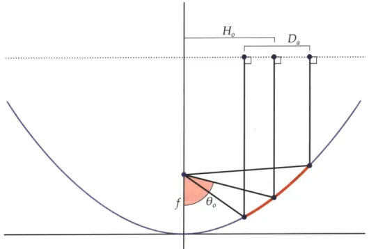
Ho

|Da

Figure 2-2: Cross-section geometry of an offset parabolic reflector with focal length

f.

The parabolic reflector covers the dark red portion of the parabola, and has diameter Da.

The boresight is offset by a distance H

0

from the centerline of the parabola, and the feed

direction is offset by 0 from the boresight. The paths of idealized incident rays are shown

as black lines.

In reality, a parabolic reflector has finite extent with the surface covering some finite

region of x and y. The curve defining the edge of this region is known as the rim of the

reflector. The rim is usually circular, in which case it could be defined by

=

(x -

xo) 2

+ (y - yo)

2

_.

_(2.15)

where Da is the diameter of the circular rim. Although an infinite reflector receives only

perfectly collimated radiation, a finite reflector instead has a beam which diverges at

some angle. This angle is the beamwidth, which is related to the wavelength A

=

c/v and

diameter as

A BW = ki-.

Da

(2.16)

The parameter k

1

is around 60 or 70, and thus this relationship can only be used to

deter-mine an approximate value for the beamwidth [4]. To find a more accurate beamwidth

for a parabolic reflector, numerical physical optics (PO) analysis is typically used. This allows for the analysis of non-elliptical rims, but does not take into account other effects, including diffraction due to the edge of the reflector and due to surface roughness, but provides a fairly accurate model in most cases [23]. The point (xo, yo) is the center of the rim. If this point is not at the origin, the reflector is known as an offset parabolic reflec-tor. An offset parabolic reflector can be used to prevent the feed antenna from obscuring the aperture of the reflector and to produce a specific angle between the feed and the boresight. One use of an offset reflector is to design a geometry with a fixed feed and a rotating reflector. This design allows the system to look in different directions without rotating the entire receiver.

Another important parameter in characterizing a parabolic reflector is the ratio be-tween the focal length and aperture diameter, or

f

/ Da. This parameter allows us to find the half-angle subtended by reflector at the focal point,

P,

as

cot;

#=

2 . (2.17)

Da ₈

_f

The angle

p

is used to match the beam of the feed antenna to the parabolic reflector. Any radiation from the feed falling outside

p

does not interact with the parabolic reflector. This is known as spillover, and a feed with significant spillover is said to over-illuminate the reflector. Over-illumination increases the sidelobe and backlobe levels of the antenna system, and decreases the beam efficiency. On the other hand, a feed which has a half-angle beamwidth significantly smaller than

#

will under-illuminate the reflector. The primary downside of an under-illuminated reflector is inefficiency in size, weight, and cost, since the region of the reflector not illuminated by the feed provides no benefit to the antenna system.

2.5.2

Horn antennas

A horn antenna is a radiator designed to match a waveguide terminal to free space.

Horn antennas are frequently used in microwave bands where the wavelengths are short enough to design a reasonably sized horn having an aperture width greater than the wavelength. A horn antenna appears with a waveguide port on one end, and flares out

or take some more complicated structure. In general, the peak gain of a horn antenna

is approximately proportional to its aperture divided by the square of the wavelength.

An approximation for a the peak gain of an optimum gain antenna, which is the antenna

with maximum gain for a given length, provided by [4] is

G 6.5A

_A

2

(2.18)

where A is the aperture area and A is the operating wavelength. The antenna beamwidth

is inversely proportional the square root of its peak gain.

L

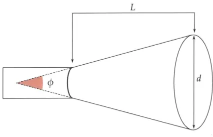
Figure 2-3: Cross-section geometry of a conical horn antenna. The feed port is on the left

side, and the antenna has aperture diameter d, length L, and flare angle

p.

A conical horn is a horn antenna with a circular aperture, shown in Figure 2-3. It

is principally characterized by two parameters: its length L and its aperture diameter d.

These two parameters further define a flare angle as

=

₂

_{arctan 2L.}

(2.19)

The flare angle has an impact on the shape of the phase front from the antenna. Generally

this is desired to be as flat as possible, which would be the case with zero flare angle, but

this does not provide optimum gain for a given antenna. The optimum gain conical horn

of length L has a diameter of d ~ v/3.125LA [23]. Realized gain is a compromise between

the optimum-gain flare angle and the required phase front flatness.

A design innovation commonly seen in high performance horn antennas is the

intro-duction of corrugations transverse to the horn flare on the interior wall of the horn. The corrugations are designed to have no effect on the boundary for radiation propagating straight out of the horn, but they reduce the propagation of radiation at other angles. Corrugated antennas are used when very low sidelobe levels are desired, typically in applications requiring a high beam efficiency. The downsides of corrugated horn anten-nas are their increased design complexity as well as manufacturing difficulties in cutting precise slots on the interior of a horn.

2.5.3 Matching the horn pattern to the reflector

To match a conical horn antenna to a reflector, we would first find the subtended angle

p

that fully illuminates the reflector. We would then determine the associated horn direc-tivity required to produce sufficiently low gain at the edges of the reflector. This would determine the horn aperture diameter. If we were designing an optimum-gain horn we could then directly determine the length. If we required a flatter phase-front across the aperture we could elongate the horn, and if we wanted to produce a spherical phase-front we could actually shorten the horn. Since both the directivity of the horn and the parabolic reflector are dependent on wavelength, a system designed for one frequency is going to behave differently when operating at a different frequency.

2.6

NAST-M

The NPOESS Aircraft Sounder Testbed -Microwave (NAST-M) is multi-band total power microwave radiometer operating near 54, 118, 183, and 425 GHz. NAST-M operates as a cross-track scanning instrument, with four feeds (one for each frequency band) looking at a flat plate reflector. The four receivers are superheterodyne, with a single sideband in the 54 GHz band and double sidebands in the other three frequency bands. NAST-M has flown on several campaigns, and has been integrated into three high-altitude science aircraft: the NASA WB-57, the Scaled Composites Proteus, and the NASA ER-2. All three of these aircraft operate at altitudes between 17km and 20 km [11]. NAST-M is intended to fly at sufficiently high altitude to measure through most of the atmosphere, providing a similar perspective to the satellite.

NAST-M provides equivalent coverage of ATMS channels 3 through 9 in the 54-GHz

band and 18 through 22 in the 183-GHz band. The purpose of the 54-GHz channels is primarily for measurement of temperature with altitude, for altitudes up to about 13 km. The 183-GHz channels are to measure humidity at varying altitudes. Channels 10 through

15 are located around 57.3 GHz. These are not represented by NAST-M, due to the fact

that their temperature weighting functions peak at altitudes between 17km and 37km. The missing channels are 10 through 15, which are located around 57.3 GHz, channel 16 at 89 GHz, channel 17 at 165 GHz, and finally channels 1 and 2 at 23.8 GHz and 31.4 GHz respectively [11, 14].

NAST-M has two external calibration reference loads: a thermally controlled hot load

at 334.0 K ± 0.1 K and an uncontrolled ambient load at 245 K ±5 K. These two loads provide good reference points for calibration as they are approximately on either end of the typical brightness temperatures measured by the system. NAST-M has an additional port located at zenith on the scan to provide a measurement of the cosmic microwave background, as seen through the atmosphere from 17km up [3].

NAST-M has a full-width at half-maximum beamwidth of 7.5', and is capable of

scanning a swath 100 km wide below the aircraft. NAST-M has flown several campaigns, collecting data over Hurricane Bonnie in 1998, underflying the NOAA-15 satellite to cor-relate data with AMSU in 1999 [1], as well as flying over convective regions in 2002 and

Chapter 3

Aircraft Sensor Design and

Development

The NPOESS Atmospheric Sounder Testbed -K-band (NAST-K) system is designed to be a fully independent passive microwave radiometer sensing near 23.8 GHz in K-band and 31.4 GHz in Ka-band. The system is designed to be deployed on an airborne platform-currently the project is designed for an initial campaign on the NASA ER-2 aircraft. The system uses a single feed horn antenna with a spinning parabolic mirror to reflect incom-ing radiation into the horn. The mirror is mounted at a 450 angle to the horn, and allows the system to view radiation in regions located cross-track to the aircraft longitudinal axis.

For this project I handled the majority of the system level design, with some guidance taken from the decisions made on NAST-M. I selected most of the components, and solicited designs for the radiometer front-end to produce a system compatible with ATMS. I did the preliminary mechanical layout of the instrument in both the WB-57, which was the original aircraft to be integrated, and later the ER-2. This included designing a preliminary model of the ER-2 wing pod from measurements I derived from photographs of the pod before actual measurements could be taken. The video amplifier was an original design I carried out for this project.

3.1 Overview

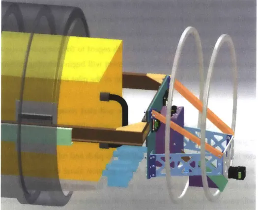
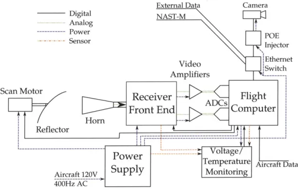
The NAST-K sensor can be divided into three major subsystems: the antenna system, the radiometer front-end, and the data acquisition system. Additionally, the sensor has several support systems including the power supply, flight computer, camera, and the voltage/temperature monitoring board. The block diagram in Figure 3-1 depicts all of the major components of the entire NAST-K system. The components of the antenna subsystem are the horn antenna, the parabolic reflector, and the scan drive motor. The radiometer front-end consists of the microwave frequency low-noise amplifiers, filters, references, and the video signal amplifiers. The data acquisition subsystem is a part of the flight computer, which contains integrated analog-to-digital converters (ADCs) for the sensor signals as well as the storage device for logging data.

NAST-K will sample each radiometer channel at a frequency of about 1 ksps, but

the data can be integrated digitally over a longer period. An integration time of 100 ms will correspond to a angular range of 7.20 at the 0.2Hz scan rate, smearing the signal over about the width of a spot. In the period of a single scan, the radiometer will have travelled about a kilometer, which means that the instrument will sample a given point in two consecutive scanning cycles. This ensures that the instrument covers the entire swath under the aircraft ground track.

3.2 Antenna assembly

The antenna assembly consists of a scanning parabolic reflector and a fixed horn antenna. The signal portion of the antenna assembly is described in detail in Chapter 4. The horn is mounted facing aft, mounted along the longitudinal axis of the aircraft. The reflector rotates the view by a fixed angle of 900, aligning the boresight with the roll plane. The specific view direction is dependent on the reflector orientation. In the default position, the system looks at nadir through a port in the aircraft skin. The reflector can be spun

by approximately 30' in either direction without the sensor view being occluded by the

aircraft skin. The reflector can also be spun 180' to orient the sensor through another port at the zenith position. This configuration allows the sensor to look down at the earth and scan out a swath of approximately 60' perpendicular to the orientation of the aircraft. As the aircraft flies this swath can be further swept into a two dimensional region along the

Figure 3-1: High-level block diagram of the NAST-K system.

aircraft ground track. The zenith port allows the sensor to look upwards to space in order

to collect a reference signal associated with the cosmic microwave background.

The scan motor is a low temperature and low pressure rated stepper motor, attached

to a digital controller to drive the motor, allowing the system to set a scan rate and read

back absolute position, or set an absolute position. The stepper motor was chosen to be

powerful enough to drive the reflector assembly directly, obviating the need for a gearbox.

This simplifies the control of the reflector and increases pointing accuracy, reducing the

backlash exhibited by a geared system. The scan assembly spins continuously as data

is collected at a constant rate, except to correct for accumulated errors between the scan

positions of the NAST-M and NAST-K reflectors. The spin rate is expected to be 0.2 Hz,

consistent with the NAST-M scanner. Coupled with the corner frequency of 300 Hz for the

receiver system (which corresponds to a 3-ms integration time) the angular "smearing"

of the signal is expected to be around 0.3', a minor distortion compared to the half-power

beamwidth of approximately

7'.

Table 3.1: Radiometer front-end performance specification Band 23.8 GHz 31.4 GHz Center frequency 23.80 GHz ± 0.01 GHz 31.40 GHz ± 0.01 GHz -3 dB bandwidth 270 MHz 180 MHz Operating band 23.53 GHz to 24.07 GHz 31.22GHz to 31.58 GHz Stop band (< -40 dB) < 22.35 GHz < 29.98 GHz > 25.25 GHz > 32.88 GHz Noise figure < 3.7dB < 3.7 dB Passband ripple

<

0.5 dB < 0.5 dB within 23.655 GHz to 23.945 GHz 31.300 GHz to 31.500 GHz

Gain at detector input > 70 dB > 70 dB

3.3 Radiometer front-end (RFE)

Aottava _{1006" ;-]}

PN23.6-31.6 (G4I LI4A 23.o-31.6 GHlz

7260/7OMttz LNA

Noise

Figure 3-2: Block diagram of the radiometer front-end (RFE)[9]

The microwave components of the radiometer front-end were designed by Boulder En-vironmental Sciences and Technology (BEST) to MIT Lincoln Laboratory specifications.

In our requirements [21] we requested two internal reference signals: a temperature con-trolled matched load and a noise diode. These signals are coupled into the receive path with a PIN diode switch and a directional coupler, respectively. Their design consists of a shared first stage LNA for both frequency bands, a power divider and filter bank to split the two bands, additional low-noise amplifiers, and finally a tunnel diode detector on each channel to rectify the microwave signal. The signals from the tunnel diode detectors are then passed to video amplifiers for additional filtering and amplification. A block

Table 3.2: Receiver noise equivalent delta-temperature (ATrms) on NAST-K and ATMS. ATMS data is based on measurements presented in [5] and

NAST-K data is based on expected noise figure and a 100 ms integration

time.

23.8 GHz band 31.4 GHz band

NAST-K Receiver Temperature (Tr) 389.8 K 389.8 K

NAST-K ATrms 0.13 K 0.16 K

ATMS Measured ATrms 0.25 K 0.31 K

ATMS Required ATrms 0.5 K 0.6 K

diagram for the RFE up to the detectors is included in Figure 3-2.

Table 3.2 compares the expected performance of the NAST-K radiometer with the measured data from ATMS. Both NAST-K channels are expected to have lower ATrms with a 100 ms integration time than ATMS. NAST-K's accuracy can be further increased

by increasing the integration time, but this has the consequence of either enlarging the

spots if the scan rate stays the same or causing gaps in the collected swath if the scanner is slowed down. Both NAST-K and ATMS are well within the ATMS specification of

ATrms = 0.5 K at K-band and 0.6 K at Ka-band [14].

3.4 Video amplifier

The video amplifier was a custom design for this project. It takes the envelope of the microwave signal, which is provided by the tunnel diode detector, and amplifies this sig-nal, low-pass filters the sigsig-nal, and differentially buffers the signal for transmission to the analog-to-digital converter on the flight computer. The first stage of the video amplifier is an instrumentation amplifier, which provides an adjustable gain with a maximum DC gain of approximately 1000, and terminates the signal from the detector with the proper input impedance of approximately 160 0. The instrumentation amplifier also isolates the signal between the RFE and the flight computer in order to avoid a ground loop through the independent RFE and flight computer power supplies. The next stage is a first-order low-pass filter with a corner frequency of 300 Hz and a fixed gain of 10. The final stage is a differential driver with an effective gain of 3.3 and an optional passive first order RC

filter on the output. There is an adjustable offset reference which is the negative input for the differential driver. This allows the zero point of the differential signal to be adjusted over a range of 2.4 V. This is to provide some flexibility in order to maximize the utiliza-tion of the ADC input range. The two adjustable parameters are changed with the use of potentiometers. These potentiometers should be replaced with fixed value resistors in operation to avoid mechanical drift of the potentiometer wiper.

The video amplifier is powered by a bipolar +5 / - 5 V supply. The supply connections are bussed between adjacent video amplifier boards in the PCB layout to permit the use of multiple video amplifier boards with a single power supply connection. NAST-K uses two video amplifiers which are not connected to each other, so the amount of cross-talk that would be caused by bussed power connections has not yet been evaluated. The signal from the tunnel diode detector is fed in through an SMA connector. The power and output signal connections are provided through 0.1 in (2.54 mm) pin headers. The external dimensions of the board are 1 in by 2 in (2.54 cm by 5.08 cm). The video amplifier schematics and board layout are included in Appendix B.

3.5 System power and grounding

3.5.1

Power Conditioning Unit

NAST-K will include a new power conditioning unit (PCU) to supply power to the system.

The PCU will include three outputs: a 28 V supply for digital electronics, a 18 V supply for the radiometer front end, and finally a 28 V supply for heaters and thermo-electric coolers. These supplies are separated in order to isolate the attached electronics from each other. A diagram of the power distribution is in Figure 3-3. The design of the PCU will be based on the NAST-M PCU. The decision was made to isolate the two power supplies in order to ensure that both instruments can still function independently.

3.5.2 Grounding

The general grounding design for the system is that of a star ground topology emanat-ing from the PCU. A ground path will follow most electrical connections, but in cases where doing so would create a ground loop, some sort of isolation is provided. The Ethernet connections are automatically isolated through the use of isolation transformers

Supply Power Connection

... . Ground Path

Endpoint Ground Isolation

RFE Heaters Isolated Jupiter Ethernet Scan

Linear +/-5V Supply DC/DC I Switch Motor

Regulator

Receiver Video _{... Flight Voltage}

Amplifiers C

n- . Computer Temperature:

E n d~.sa. ... e

... _... M onitor

Figure 3-3: NAST-K power connections.

as required by the 100BASE-TX standard. The control signals for RFE components are optoisolated on the RFE side. Finally, the signal path from the RFE through the video amplifiers out to the flight computer had the potential for a ground loop, but this was mitigated by isolating the signal at the instrumentation amplifiers at the inputs of the video amplifiers. There is a very weak ground connection through a high value resistor between the two sides. Further, the power supply for the video amplifiers is itself isolated, ensuring that the ground reference for the video amplifiers is that of the flight computer and consequently the A/D converter.

3.5.3

EMI

The analog signals from the video amplifier are fed through individually-shielded twisted-pair cables. This is to minimize the possibility of external interference in the cable run between the RFE enclosure and the flight computer enclosure. In general, all enclosures

should be metal-clad with metal shielded feed-throughs.

3.6 Flight computer

The NAST-K flight computer is responsible for collecting sensor data and controlling most of the other systems in the sensor. The flight computer has an on-board analog-to-digital converter which samples the outputs from the video amplifiers. It also collects temperature and voltage data from the monitoring board. It sends commands to the scan . .. .... - -__ ---_ - ...

motor assembly to control the reflector position. It also sends commands to the noise

diode and PIN diode switch in the RFE in order to select the noise diode or matched load

calibration references for regular instrument calibration. Finally, the computer records

data from the aircraft bus, receives control signals from and transmits status signals to

the aircraft, communicates with NAST-M for reflector synchronization, and operates the

camera.

3.6.1

Hardware

The flight computer is a PC/104 form-factor single board computer with an 486

archi-tecture CPU operating at 800 MHz with 256 MB of on-board DRAM, with a rated power

consumption of 5.4W. The computer is manufactured by Diamond Systems under the

name Helios[8]. For our application we have added a 2GB IDE flash drive, as well

as a Compact Flash (CF) card. The board contains an integrated 16-bit 250 ksps

self-calibrating analog-to-digital converter with 8 differential inputs (of which we are using

two for the K- and Ka-band video amplifier signals). Additionally, the board has digital

general purpose I/O (GPIO) lines, several serial ports, an on-board Ethernet adapter, and

keyboard/video/mouse connections. The computer takes supply voltages of +5V and

+12V which are provided by a power supply board connected to the PC/104 ISA bus.

The power supply board takes a single +28 VDC input.

Figure 3-4: Flight computer enclosure I/O panel. [8]

One of the flight computer serial ports is being used for communication with the embedded environmental monitor (EEM) (see Chapter 5). Another will be used for com-munication with the aircraft data bus, as well as another to receive data from the NAST-M

GPS module. The Ethernet connection allows for data retrieval on the ground, as well as

communication with the camera and with NAST-M. The keyboard and mouse PS/2 ports as well as the VGA port are made available to operate the computer in the event that it is not functioning properly and is not reachable over the network. The GPIO lines are used to read the pilot control signal as well as to send power/fail status back to the pilot. Finally, several of the GPIO lines are fed to the RFE to control the PIN switch and noise diode output for periodic instrument calibration.

3.6.2

Operating System

The flight computer hardware is based on the x86 architecture, so we chose a general purpose Ubuntu Linux distribution on the computer. This would provide easy access to a variety of software as well as simple software development on a separate Linux-based computer. The normal server (no-GUI) version of Ubuntu Linux 10.04 was installed on the flight computer, but the processor could not boot the kernel due to lack of support for certain instruction set exceptions. This was resolved by compiling the kernel from source on the development computer and targeting it to the specific instruction set implementa-tion of the CPU, and then replacing the installed kernel with the custom-compiled one. Compiling the kernel provided several advantages. First, we could remove support for a lot of unused hardware, reducing the required space considerably. We could add support for the specific hardware on our board, namely the A/D converter and the network card, both of which were not supported by the default kernel. Finally, we were interested in running our operational program at a real-time priority to guarantee timing performance, and we could accomplish this by enabling real-time extensions in the configuration.

There are two storage devices available on the flight computer. The IDE flash disk has the OS installed on it, and in operation will only be mounted read-only. This is accomplished by creating a RAM disk on system boot and using AUFS to lay the RAM disk over the read-only root file system. Any changes to root will be changed in the RAM disk and not the permanent disk. This operation is designed to be transparent to any software running on the operating system, so the software will be able to make changes