HAL Id: hal-01361778
https://hal.archives-ouvertes.fr/hal-01361778
Submitted on 12 Sep 2016HAL is a multi-disciplinary open access archive for the deposit and dissemination of sci-entific research documents, whether they are pub-lished or not. The documents may come from teaching and research institutions in France or abroad, or from public or private research centers.
L’archive ouverte pluridisciplinaire HAL, est destinée au dépôt et à la diffusion de documents scientifiques de niveau recherche, publiés ou non, émanant des établissements d’enseignement et de recherche français ou étrangers, des laboratoires publics ou privés.
Optimization of metabolite detection by quantum
mechanics simulations in magnetic resonance
spectroscopy
Giulio Gambarota
To cite this version:
Giulio Gambarota. Optimization of metabolite detection by quantum mechanics simulations in magnetic resonance spectroscopy. Analytical Biochemistry, Elsevier Masson, 2017, 529, pp.65-78. �10.1016/j.ab.2016.08.019�. �hal-01361778�
1
Optimization of metabolite detection by quantum mechanics simulations
in magnetic resonance spectroscopy
Giulio Gambarota1, 2
1
Université de Rennes 1, LTSI, Rennes, F-35000, France
2
INSERM, UMR 1099, Rennes, F-35000, France
Running Head: Quantum mechanics simulations in magnetic resonance spectroscopy
Corresponding author:
Giulio Gambarota, Ph.D. Professor
INSERM, U1099
Université de Rennes 1, LTSI 35043 Rennes, France
tel: 02 23 23 48 49
email: [email protected]
Word count: xxxx
Number of figures and tables: 6 Number of references: 120
2
Abstract
Magnetic resonance spectroscopy (MRS) is a well established modality for investigating tissue metabolism in vivo. In recent years, many efforts by the scientific community have been directed towards the improvement of metabolite detection and quantitation.
Quantum mechanics simulations allow for investigations of the MR signal behaviour of metabolites; thus, they provide an essential tool in the optimization of metabolite detection. In this review, we will examine quantum mechanics simulations based on the density matrix formalism. The density matrix was introduced by von Neumann in 1927 to take into account statistical effects within the theory of quantum mechanics. We will discuss the main steps of the density matrix simulation of an arbitrary spin system and show some examples for the strongly coupled two spin system.
Keywords: Keywords: Quantum Mechanics simulations; Density Matrix; Magnetic
Resonance Spectroscopy; Metabolites; Strongly coupled spin systems. .
3
Introduction
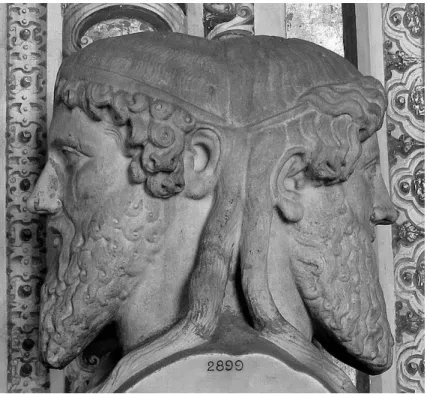
Nuclear magnetic resonance (NMR) is a Janus-faced physical phenomenon. Janus was a Roman god, with no equivalent in the Greek mythology. He was the god of the beginnings -the first month of -the year, January, was named after him [1]. Janus was typically depicted with two faces (Figure 1). Similarly to this Roman god, the NMR phenomenon has two diametrically opposed faces. Since the very beginning, at the time of its discovery NMR was described in two completely different ways: Edward Purcell, at Harvard, pictured the NMR as quantum transitions between energy levels whereas Felix Bloch, at Stanford, viewed the NMR as the precession of a magnetization vector obeying the laws of electromagnetism [2-4]. Thus, two diametrically opposed views to describe the same phenomenon: quantum mechanics on one hand, classical physics on the other hand. An excellent account of the NMR discovery can be found in the article entitled "Quantum states and precession: The two discoveries of NMR" written by John Ridgen [5].
Within the historical context of the NMR discovery [6, 7] we cannot avoid to mention the lesser-known NMR pioneer Cornelius Gorter and his "ingenious early attempts" (as Bloch later called them [8]) to observe the magnetic resonance phenomenon [9, 10]. The Dutch physicist tried first in 1936 to detect MR in LiF using a calorimetric method, in order to measure the heating caused by energy absorption at the resonance condition. Then, he tried in 1942 to observe the resonance employing a dispersion method; again with little luck. With respect to the unsuccessful experiments of Gorter, Van Vleck later recalled : "The real difficulty arose from the fact that he used too much power and too pure materials, things that are advantages in most physical experiments [...] If Gorter had tried to detect the resonance in ordinary tap water [...] he might have succeeded." [11].
In this review we will focus on the quantum mechanics viewpoint of the magnetic resonance phenomenon. We will examine the role of quantum mechanics -and more precisely the density matrix formalism- in the optimization of metabolite detection in vivo by magnetic resonance spectroscopy (MRS). Measurements of metabolites in vivo present a number of challenges, mainly related to 1) the intrinsically low-sensitivity of MRS and 2) the spectral overlap among resonances of different metabolites. Quantum mechanics simulations allows for investigations of the MR signal behaviour of metabolites. These simulations aid in 1) identifying the optimal acquisition parameters for in vivo measurements and 2) developing novel acquisition schemes that could further improve metabolite detection and quantification.
4
Magnetic resonance spectroscopy
Magnetic resonance spectroscopy is a well established modality for investigating tissue metabolism in vivo. 1H MR spectra can be routinely obtained in clinical settings with MRI systems operating at the field strength of 1.5 T and 3 T, using standard equipment. In the next paragraphs we will briefly review the most common applications of 1H MRS in clinical and research scenarios -cautiously avoiding the perennial question regarding the clinical utility of
1
H MRS [12-16]. The objective here is to identify the specific cases (which organ/tissue? which metabolite?) where the quantum mechanics approach is necessary.
Nowadays in vivo 1H MRS is mostly performed on brain, prostate, muscle, liver and breast. Undoubtedly, brain MR spectra display the largest number of metabolites compared to any other organ/tissue. The major metabolites in brain include N-acetylaspartate, creatine, choline, glutamate, glutamine, myo-inositol, taurine, GSH and GABA [13, 14]. A considerable overlap among the resonances of these metabolites is present. A number of editing methods were originally proposed, more than 20 years ago, with the focus on the quantification of GABA [17-20]; the investigation of new methods to improve quantification of GABA (and other brain metabolites) is still a current object of research [21]. In general, the driving force has been the investigation of brain function and metabolism [22-24], also with specific interest to study efficacy of therapy, as in the case of GABA tissue levels in patients with epilepsy, for instance [18, 25]. At the field strength of clinical MRI systems, many brain metabolites (glutamate, glutamine, myo-inositol, etc. [26]) behave as strongly coupled spin systems -we will see the exact definition of ‘strongly coupled’ later on. At this stage we can say that the quantum mechanics approach is needed to simulate the signal behavior of these "particular" spin systems; in this context, the density matrix formalism has been essential in the optimization of a number of metabolites present in brain.
Another organ that has attracted the attention of MR spectroscopists from the very beginning of clinical MRS applications is the prostate, for the diagnosis of prostate cancer [27, 28]. The
1
H MR spectrum of healthy prostate tissue reveals the resonances of citrate and choline; a reduction in citrate and an increase in choline is observed in cancer tissue. As in the case of certain brain metabolites, citrate requires quantum mechanics modelling to precisely simulate the MR signal in order to determine the optimal pulse sequence and pulse sequence parameters [29, 30].
The 1H MR spectrum of muscle tissue includes resonances of choline-containing compounds, creatine, taurine and two groups of lipid signals: the intramyocellular (IMCL) and
5
extramyocellular (EMCL) lipids [31, 32]. There is a frequency shift between the IMCL and EMCL, due to the magnetic susceptibility difference between the spherical and cylindrical compartments of the IMCL and EMCL. None of the main metabolites typically found in muscle requires the quantum mechanics approach for proper detection. Same conclusion applies to the MR spectrum of liver tissue, which includes resonances of choline-containing compounds and the resonances of the intrahepatocellular lipids [33, 34]. It should be pointed out that taurine (present in muscle) is a strongly coupled spin system; however, it could be detected without the need of quantum mechanics simulations.
In MRS of breast, similarly to the case of prostate, the main focus has been on the diagnosis of cancer, with choline-containing compounds being the biomarker of interest [35-37]. Recently, the role of lipids in breast cancer has also attracted the attention of researchers [38] and a number of 1H MRS studies have been dedicated to the measurement of breast adipose tissue composition, as a potential cancer biomarker [39-41]. Overall, for the detection of the main metabolite of interest in breast MRS (choline) there is no need of quantum mechanics simulations.
Given the growing interest in the measurement of lipid composition in vivo, a quick clarification on quantum mechanics simulations applied to lipid resonances is necessary. The long lipid hydrocarbon chains are substantially more complex than the smaller molecules of metabolites. Some moieties of the hydrocarbon chains behave as strongly coupled spin systems, and thus quantum mechanics simulations are required for investigations of the MR signal of lipid resonances. Only a handful of studies have been dedicated to this subject [42-45]. To reduce the complexity of the problem, a simplified model with only a subset of spins (seven or ten) was considered in the simulations. Due to the lack of precise knowledge of the spin system parameters and relaxation effects, simulations of lipid resonances have been to date only partially successful.
6
Quantum mechanics
Quantum mechanics was developed during the first quarter of the twentieth century to investigate and explain a number of phenomena occuring on the time and spatial scale of atomic processes [46]. One of these phenomena was the black-body radiation, which couldn’t be explained by the laws of classical physics. The solution to this problem came from Max Planck. In 1900 he put forward the hypothesis of the "quantum of action": the energy is quantized, that is, it appears in discrete, quantized values; this idea could be considered as the beginning of quantum mechanics. In a letter to the american physicist Robert Wood, Planck referred to this hypothesis as a "desperate hypothesis" [47, 48].
Another milestone was set with the investigation of the photoelectric effect; similarly to the case of the black-body radiation, classical physics failed to explain this phenomenon. In his annus mirabilis (1905) Albert Einstein provided the solution by introducing the "quantum of light". Among the last milestones of quantum mechanics was the development of the wave equation by Schroedinger in 1927:
𝑖ħ𝑑𝜓
𝑑𝑡 = 𝐻𝜓
where 𝜓 is the wavefunction, 𝐻 is the Hamiltonian, ħ the Planck constant. The wave formulation of quantum mechanics stated that a particle in the microscopic world can be described by a wavefunction, which represents the quantum state of the particle and obeys the Schroedinger equation; the Hamiltonian contains all the information related to the energy interactions that characterize the given system. A simple example is the so-called particle in a box (that is, the model of an eletron in a potential well): by solving the Schroedinger equation we obtain the wavefunction and all the physical quantities characteristic of the particle in this scenario.
Two atypical meetings are noteworthy in the development of quantum mechanics: the Solvay Conferences of 1911 and 1927. These conferences were organized by Ernest Solvay, a Belgian chemist and philanthropist who became rich with the revenues from his patent on the ammonia-soda process (or Solvay process); he decided to organize a series of meetings where scientists could share and discuss scientific results and ideas. The participation at these meetings was restricted to a limited number of invited scientists. The first Solvay Conference, entitled "La théorie du rayonnement et les quanta", took place in 1911 when the overall formalism of the quantum mechanics was still at its beginning. The first words of the Conference Proceedings (in French [49]) read: "Un Conseil scientifique (sorte de Congrès privé) s'est réuni à Bruxelles, sous les auspices de M. Ernest Solvay, du 30 octobre au 3
7
novembre 1911, dans le but de discuter une série de points controversés des théories physiques modernes." Thus, the first Solvay Conference was "a kind of private congress" that took place in Bruxelles "with the objective to discuss a number of controversial issues of the modern physics theory". In the opening speech, Hendrik Lorentz referred to "the desperate hypothesis" of Planck as "the beautiful hypothesis": "[…] la belle hypothèse des éléments d’énergie, émise pour la première fois par M. Planck et appliquée à de nombreux phénomènes par M. Einstein, M. Nernst et d’autres, a été un précieux trait de lumière. Elle nous a ouvert des perspectives inattendues et même ceux qui la regardent avec une certaine méfiance doivent reconnaître son importance et sa fécondité. Elle mérite donc bien d'ètre le sujet principal de nos discussions […]’. Lorentz highlighted the relevance of Planck’s idea, "this sudden illumination", when stating that "even those who are skeptical about this hypothesis should recognize its importance. This hypothesis truly deserves to be the main subject of our discussion […]".
By 1927, the year of the fifth Solvay Conference entitled "Électrons et photons", quantum mechanics had reached a mature state with the development of the wave mechanics and Schroedinger equation. Niels Bohr, Max Born, William Lawrence Bragg, Léon Brillouin, Arthur Compton, Marie Curie, Louis de Broglie, Peter Debye, Paul Dirac, Paul Ehrenfest, Albert Einstein, Werner Heisenberg, Hendrik Kramers, Paul Langevin, Hendrik Lorentz, Wolfgang Pauli, Max Planck and Erwin Schroedinger were among the participants of this meeting [50]. It is hard to think of any other meeting in the history of science that could compare to this one, in terms of concentration of geniuses.
In the introductory courses of quantum mechanics we learn to solve the Schroedinger equation for different scenarios, in order to obtain the wavefunction and calculate the physical quantities of interest in a given physical system. Here we need to take a step further. In the field of MRS we are interested in the magnetic properties of a particle, specifically the magnetization (spin) of the hydrogen atom nuclei (i.e., protons). Certainly, the quantum state of a spin is also described by a wavefunction; on the other hand, to simulate the MR signal we need to introduce a new, additional concept since the wavefunction alone is not sufficient for achieving our goal. This new concept is the so-called density matrix; now, why do we need the density matrix? The signal in an MRS experiment originates from many nuclei of hydrogen atoms, that is, from an ensemble of spins. In general, when we investigate the behaviour of an ensemble of particles and we do not have the exact knowledge of the state of each individual particle, we need to use statistical approaches. This occurs in classical physics
8
as well as in quantum mechanics. In the case of phenomena which obey the laws of classical physics, we employ the classical statistical mechanics to investigate the physical properties of the ensemble. Likewise, in the case of quantum mechanics phenomena, we need to enter the field of quantum statistical mechanics to combine the quantum mechanics with the statistical approach. The density matrix was introduced by von Neumann in 1927, with Dirac further developing this concept in 1929, to take into account statistical effects/phenomena within the theory of quantum mechanics [51, 52]. The density matrix contains all the statistical information about the status of the ensemble. It should be pointed out that the density matrix is actually a quantum mechanical operator, thus the proper nomenclature is "density operator"; on the other hand, it is typically referred to as density matrix, since its most common representation is in a matrix form.
In the following paragraphs, we will introduce the mathematical definition of the density matrix and the equation that governs the time evolution of the density matrix. We will use the Dirac notation, that is, the symbols " < | " and " | > " which are called "bra" and "ket", respectively; the bra is the conjugate transpose of the ket. These symbols were introduced by Dirac (with a bit of humor in choosing the names bra-ket) to represent generic vectors; in the quantum mechanics context, these vectors are the wavefunctions which describe the quantum states.
In general, a spin system can be in quantum state |> that is a superposition of basis functions (eigenstates); this quantum state can therefore be written as a linear combination of eigenstates |𝜑𝑛 > with coefficients 𝑐𝑛:
|> = ∑ 𝑐𝑛 |𝜑𝑛 > 𝑛
and in this case, the system is said to be in a pure state |> . The expectation value (i.e., mean value) of a physical quantity 𝐴 (described by the quantum operator denoted 𝐴) is given by the formula:
< 𝐴 > = < | 𝐴 | >= ∑ 𝐴𝑛𝑛′𝑐𝑛∗𝑐𝑛′
𝑛𝑛′
where 𝐴𝑛𝑛′ are the elements of the matrix that represents the operator 𝐴.
When considering an ensemble of spins, the quantum state of the ensemble could consist of spins in different pure states, |1 >, |2 >, … , |𝑖 >, with each state having a given
statistical weight 𝑝𝑖. In this situation, the systems is said to be in a mixed state |> and this quantum state is written as:
9
|> = ∑ 𝑝𝑖 |𝑖 > 𝑖
In the scenario of a mixed state, we can calculate the expectation value of a physical quantity 𝐴 by taking into consideration the different states and their statistical weight 𝑝𝑖 :
< 𝐴 > = < | 𝐴 | >= ∑ 𝑝𝑖 < 𝐴 >𝑖 𝑖 = ∑ 𝑝𝑖∑ 𝐴𝑛𝑛′𝑐𝑛𝑖∗ 𝑛𝑛′ 𝑐𝑛′𝑖 𝑖 = ∑ 𝐴𝑛𝑛′∑ 𝑝𝑖𝑐𝑛𝑖∗ 𝑖 𝑐𝑛′𝑖 𝑛𝑛′
Now, a square matrix 𝜎 -the density matrix- can be defined and the density matrix elements are equal to:
𝜎𝑛𝑛′ = ∑ 𝑝𝑖𝑐𝑛𝑖∗
𝑖
𝑐𝑛′𝑖
As a consequence, the density matrix operator can be written as follows: 𝜎 = ∑ 𝑝𝑖 | 𝑖 >
𝑖
< 𝑖 |
Using the relations above, the expectation value of physical quantity 𝐴 is: < 𝐴 > = ∑ 𝐴𝑛𝑛′∑ 𝑝𝑖𝑐𝑛𝑖∗ 𝑖 𝑐𝑛′𝑖 = 𝑛𝑛′ ∑ 𝐴𝑛𝑛′ 𝑛𝑛′ 𝜎𝑛𝑛′ = 𝑇𝑟(𝐴𝜎)
where "𝑇𝑟" represents the trace operation. Thus, from the knowledge of the density matrix it is possible to determine the value of any physical variable 𝐴 of the system using the above relation, i.e., by calculating the trace of the product of the density matrix and the operator corresponding to the physical quantity of interest.
The elements of density matrix have the following physical meaning: the diagonal element 𝜎𝑖𝑖 represent the probability that the system is in the state |𝑖 >; that is, 𝜎𝑖𝑖 provides the population of spins in the state |𝑖 >. The off-diagonal elements 𝜎𝑖𝑗 are terms that connect
two different states |𝑖 > and |𝑗 >; these off-diagonal elements are the so-called
coherences of the states |𝑖 > and |𝑗 >.
Starting from the Schroedinger equation, it is possible to derive the equation that governs the time evolution of the density operator, the Liouville - von Neumann equation:
𝑖ħ𝑑𝜎(𝑡)
𝑑𝑡 = [𝐻(𝑡), 𝜎(𝑡)]
In this equation, the square-bracket symbol "[ ]" represents the so-called commutator symbol defined as [𝜎, 𝐻] = 𝜎𝐻 − 𝐻𝜎. The Liouville - von Neumann equation for the density matrix is the equivalent of the Schroedinger equation for the wavefunction. The solution of the Liouville - von Neumann equation for a time-independent Hamiltonian is:
10
where 𝜎(0) is the density matrix at time = 0 and 𝜎(𝑡) is the density matrix at time 𝑡. Thus this formula allows us to evaluate the time evolution of the density matrix, once the initial density matrix and the Hamiltonian are known.
Finally, it should be noted that the density matrix is the quantum mechanical analogue to the classical ensemble distribution function, in the sense that it can be used in the same way as the classical distribution function to define the average values of any physical quantity. In the classical case, these averages are weighted means; in quantum mechanics these average are defined as the trace of the product of the density matrix and the operator of interest. In the section Density matrix simulations we will provide some examples of application of the density matrix to the MR signal simulations. In the next section we will consider the classification of spin systems into weakly coupled and strongly coupled systems.
11
Weakly coupled and strongly coupled spin systems
In order to simulate the MR signal behaviour of a given metabolite, we need to know the proton chemical shifts and 𝐽 coupling constants. First, we will examine the physical phenomenon behind the chemical shifts and 𝐽 coupling constants. Protons of different hydrogen atoms in a metabolite might precess at different frequencies (chemical shifts), as the different protons might experience different local magnetic fields. The origin of the chemical shift is related to the fact that the applied static magnetic field Bo will induce electron currents in the molecule; these currents produce local magnetic fields which are on the order of 10-6 times the external field, that is, we deal with resonance frequency differences of parts per million (ppm). In addition, proton MR spectra of many metabolites display a structure which cannot be explained only in terms of chemical shifts within molecules. The additional splitting of the MR peaks from each proton into multiplets is related to the (indirect) interaction between nuclei via the bonding electrons. The difference between any two adjacent components of a multiplet is equal to the value of the 𝐽 coupling constant.
Once the chemical shifts and 𝐽 coupling constants of a given metabolite are known, it is possible to determine whether the metabolite should be modelled as a ‘weakly’ or ‘strongly’ coupled spin system, at a given field strength. The distinction between the weakly and strongly coupled systems is based on the following criterion: when the difference between the chemical shifts is much larger than the 𝐽 coupling constant, the spin system is weakly coupled. In other words, two spins with chemical shifts of 𝑣1 and 𝑣2 and a 𝐽 coupling constant equal to 𝐽12 are weakly coupled if |𝑣1− 𝑣2| ≫ 𝐽12. A typical example of a weakly coupled spin
system is lactate [26]: the CH3 protons resonate at 1.3 ppm and the CH protons resonate at 4.1
ppm, with the 𝐽 coupling constant being 7 Hz. At 1.5 T, the chemical shift difference between the CH3 and CH protons is ~180 Hz >> 7 Hz, so the spin system of lactate can be modelled as
a weakly coupled system. When the difference between the chemical shifts is not much larger than the 𝐽 coupling constant, that is, the criterion |𝑣1− 𝑣2| ≫ 𝐽12 is not satified, the spin system is strongly coupled. A typical example of a strongly coupled system is citrate. The citrate protons resonate at two frequencies with the difference being 0.146 ppm and the 𝐽 coupling constant is 15 Hz. It should be pointed out that different values of chemical shifts and 𝐽 coupling constant of citrate could be found in the literature; it has been shown that these values change with cation concentration and pH [53]. At 1.5 T the value of the chemical shift difference 𝛿 is 9 Hz, which is not larger than 𝐽 coupling constant; as a consequence at 1.5 T we need to model citrate as a strongly coupled spin system. Same argument applies at the
12
field strength of 3 T: the chemical shift difference ( = 18 Hz) is not much larger than the 𝐽 coupling constant (15 Hz, as the 𝐽 coupling constant value is independent of the magnetic field strength). Now we examine the case of citrate at the field strength of 11.7 T. The chemical shift difference is 𝛿 = 70 Hz, which is certainly larger than the 𝐽 coupling constant. However, despite the fact that 𝛿 is more than four times the 𝐽 coupling constant, we still cannot classify citrate as a weakly coupled spin system. Indeed, it has been shown that even at 11.7 T the MR signal of citrate display a signal behaviour (i.e., coherence transfer effects during interpulse delays) which could occur only in strongly coupled spin systems [54]. Thus, with respect to the criterion of weakly vs strongly coupled, one should pay attention to the fact that a spin system is weakly coupled only when the difference between the chemical shifts is much larger than the 𝐽 coupling constants. In all other cases, the spin system should be classified as strongly coupled.
Why is this classification ‘weakly vs strongly coupled’ important? It is important because in the case of weakly coupled spin systems it is possible to use the approach of the product operator formalism [55, 56], which was introduced in 1983 as a simplification of the fully quantum-mechanics formalism of the density matrix. The product operator formalism is a convenient description for weakly coupled spin systems: it introduces simple rules to account for the effects of chemical-shifts, 𝐽 coupling and radiofrequency pulses. The product operator formalism is a rigorous method to calculate the signal of spin systems; its drawback, however, is that it is valid only for weakly coupled spin systems. Thus, when dealing with strongly coupled spin systems, we need to resort to quantum mechanics tool introduced by von Neumann in 1927, i.e., the density matrix. Finally, one should also note that in addition to weakly vs strongly coupled spin systems, some spins in a number of metabolites behave as singlets (that is, uncoupled spins); in this case, the Bloch equations could be used to simulate the signal behaviour. For instance the CH2 protons of glycine, which yield a singlet at 3.55
13
The need of MR signal simulations for in vivo MRS
The challenges of in vivo 1H MRS are related to the low tissue levels of metabolites (~mM, "low" relative to the sensitivity of MRS), the limited amount of time available for in vivo experiments and the spectral overlap among resonances. Even at a high field strength (7 T for MR research systems dedicated to human studies) spectral overlap still hampers the quantification of a number of metabolites.
Many different approaches have been proposed throughout the years for optimizing metabolite detection. From a pragmatic point of view, these approaches can be classified in two main groups: 1) approaches dedicated to the parameter optimization of the STEAM (stimulated echo acquisition mode) and PRESS (double spin-echo point resolved spectroscopy) sequences [57-81], the two commonly used pulse sequences that are readily available on clinical scanners and 2) approaches focused on the development of new pulse sequences; some examples are provided in [17-21, 82-93].
Another way of classifying the different optimization methods is based on the spin system characteristics of the metabolite of interest: that is, whether the metabolite of interest is represented by a coupled or uncoupled spin system. When the metabolite of interest has coupled resonances with the overlapping (confounding) resonance being a singlet –such as the GABA resonance underneath the singlet of creatine, for instance– a number of methods (based on interpulse-delay optimization, difference spectroscopy editing, multiple quantum coherence editing, etc) have been implemented in vivo, see for instance [57-93]. A different situation occurs when the metabolite of interest is a singlet and the overlapping resonance is a coupled spin system –for instance the glycine singlet resonance underneath the myo-inositol. In this case, one option is to use a long echo time (or multiple echo times) in order to minimize the MR signal of the coupled resonance, by exploiting the intrinsic 𝐽 coupling-induced dephasing [94-96]. Another option is to simulate the 𝐽 modulation of the coupled resonance and choose a relatively short echo time that minimizes the signal intensity of the coupled resonance, see for instance [97, 98]; in the latter option, the losses due to T2 relaxation are also minimized.
In general, regardless of the specific approach implemented to quantify a given metabolite, it is essential to perform signal simulations to determine the optimal pulse sequence and sequence parameters. The density matrix formalism allows for the determination of the MR signal of spin systems, including the strongly coupled systems. The analytical calculations using the density matrix are very cumbersome even for a strongly coupled two-spin system.
14
Examples of these calculations are provided in a number of studies [29, 30, 54, 99-101]. In particular, for the two-spin system it is still fairly feasible to account analytically for the effects of the 180° pulses, as in the PRESS sequence. The calculation for the STEAM sequence on the other hand is quite prohibitive [30] since the 90° pulses and magnetic field gradients exacerbate the already complicated nature of the analytical approach. In spin systems with three or more spins, analytical calculations would easily take months of work. Thus, it is crucial to adopt the approach of computer simulations to obtain the MR signal of a strongly coupled spin system. In the next section, we will consider in detail the density matrix simulations of strongly coupled spins systems.
15
Density matrix simulations
Theory
There are a number of books [102-107] and articles [108-117] with a detailed description of the density matrix formalism applied to MR spectroscopy problems. The goal here is to guide the reader through the main steps of the density matrix simulations, providing the general guidelines, a certain insight and some details. We start with the simulation of a strongly coupled two-spin system. This specific case was among the first applications of the density matrix approach to in vivo MRS: it was used for optimizing the detection of citrate, metabolite of interest in the diagnosis of prostate cancer. The strongly coupled two-spin system also represents the ideal spin-system prototype to introduce the basic concepts of density matrix simulations: indeed, it is the simplest spin system that contains all the necessary ingredients, i.e., the chemical shift and 𝐽 coupling constant. The notation often adopted to indicate each spin uses the letters of the alphabet: two strongly coupled spins are denoted by letters that are close to each other in the alphabet (A and B, for instance); whereas two spins that are weakly coupled are denoted by letters that are far from each other (AX spin system). For instance, the spin system of citrate -which can be modelled as a strongly coupled two-spin system- is called an AB spin system, whereas for lactate the spin system is an AX3 system.
The first step consists in evaluating the Hamiltonian of the spin system. As we said previously, a quantum system is defined by its Hamiltonian, which contains all the energy interactions of the given system. In order to write down the Hamiltonian we need to know the values of the chemical shifts and 𝐽 coupling constants. For an AB spin system, we denote 𝜔𝐴 and 𝜔𝐵 the chemical shifts of the spin A and B, respectively, and 𝐽𝐴𝐵 the coupling constant. We use the angular frequency units for the Hamiltonian parameters, 𝜔 and 𝐽, so that we can write the Hamiltonian in angular frequency units, with the Planck constant set equal to unity; furthermore, since we restrict our discussion to the 1H MRS, we deal only with spins having quantum number of ½.
The energy interactions of a coupled two-spin system are: 1) the Zeeman interaction, which represents the interaction between the spins and the applied magnetic field and 2) the 𝐽 coupling interaction, which accounts for the electron-mediated interaction between the (nuclear) spins. The 𝐽 coupling interaction is also called "indirect coupling" to distinguish it from the "direct", dipole-dipole interaction between spins. Here we can neglect the dipolar
16
interaction, since it averages to zero under the assumption of fast isotropic molecular reorientation.
The Zeeman interaction is written as the product of the chemical shift and the z-component of spin angular momentum operator (the static magnetic field is applied, as usually, along the z direction). The 𝐽 coupling interaction is equal to the scalar product of the angular momentum operators of the two spins -this is the reason why the 𝐽 coupling interaction is often referred to as "scalar" coupling. Historically, the angular momentum operators of a two-spin system (the A and B spins in this case) have been denoted by the letter 𝐼 and 𝑆. Now we can write the Hamiltonian:
𝐻 = 𝜔𝐴𝐼𝑧+ 𝜔𝐵𝑆𝑧+ 𝐽𝐴𝐵𝐼 ∙ 𝑆
where to summarize 𝜔𝐴 and 𝜔𝐵 are the chemical shifts of the spin A and B, respectively,
𝐽𝐴𝐵 is the 𝐽 coupling constant, 𝐼 and 𝑆 are the spin angular momentum operators, 𝐼𝑧 and 𝑆𝑧 are z-components of the spin angular momentum 𝐼 and 𝑆, respectively. We could also refer to this Hamiltonian as the "internal" Hamiltonian, since it depends only on the characteristics of the spin system. Once the internal Hamiltonian is known, by diagonalization of the Hamiltonian matrix it is possible to calculate the energy levels and determine the position in the spectrum of the resonance peaks. More details could be found in the literature; for instance in the books by Pople [102] and Corio [103], as well as in the review paper by Corio [109], many examples of spin systems (AB, A2B, A3B, A3B2, ABC, ABX…) are discussed in depth; the
spin system eigenvalues and eigenfunctions, their resonance frequencies and relative intensities are tabulated in great detail.
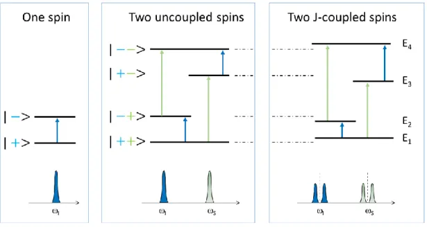
In Figure 2, a schematic representation of the energy levels in a one-spin system and a two-spin system, is shown. In the one-two-spin system we have two two-spin states: i) the state denoted as |+>, where the spin is aligned with the field and ii) the state denoted as |−>, with the spin aligned against the field; in this latter state, the spin has a higher energy than in |+>. Thus, the one-spin system has two energy levels and one transition, which yields one resonance peak (Figure 2, left panel).
For a two-spin system we have four spin states, which correspond to 1) two spins aligned with the field | + +>, 2) two spins aligned against the field | − −>, and 3) & 4) one spin aligned with and the other aligned against the field, | − +> & | + −>, respectively. Each state (| + +>, | − +>, | + −>, | − −>) is characterized by its energy level (E1, E2, E3, E4,
17
According to the selection rules of quantum mechanics (change in the spin system quantum number = ±1) there are the four allowed transitions, which are indicated by the arrows (Figure 2): E1E2, E1E3, E2E4 and E3E4.
In the case of two uncoupled spins (Figure 2, center panel), the transition E1E2, yields the
same resonance peak as the transition E3E4; furthermore, the transition E1E3, yields the
same resonance peak as the transition E2E4. The 𝐽 coupling modifies the value of the energy
levels: the two singlets become now two doublets (Figure 2, right panel), with the effect of the 𝐽 coupling on the energy levels becoming more important when the spins are strongly coupled.
In addition to the four allowed transitions, there are two ‘forbidden’ transitions: E2E3, and
E1E4, where the change in quantum number is zero and 2, respectively; for this reason,
these transition are denoted as zero-quantum and double-quantum transitions.
With regard to the spin system Hamiltonian: in a previous section, we have discussed the difference between the weakly coupled and strongly coupled spin systems. Now we will discuss the difference between the Hamiltonian of the weakly coupled and the strongly coupled two-spin system.
In the strongly coupled system, the scalar interaction term 𝐽𝐼 ∙ 𝑆 is the scalar product of the two angular momentum operators, that is:
𝐽𝐼 ∙ 𝑆 = 𝐽(𝐼𝑥𝑆𝑥+ 𝐼𝑦𝑆𝑦+ 𝐼𝑧𝑆𝑧)
In the weakly coupled system, we can use the approximation that neglects the off-diagonal terms; in other words, the simplification of the scalar coupling yields:
𝐽𝐼 ∙ 𝑆 ≈ 𝐽(𝐼𝑧𝑆𝑧)
Thus, the Hamiltonian of a weakly coupled two-spin system (an AX system) is written as: 𝐻 = 𝜔𝐴𝐼𝑧+ 𝜔𝑋𝑆𝑧+ 𝐽𝐼𝑧∙ 𝑆𝑧
where 𝜔𝐴 and 𝜔𝑋 are the chemical shifts of the spin A and X, respectively, 𝐽 is the coupling constant, 𝐼𝑧 and 𝑆𝑧 are z-components of the spin angular momentum 𝐼 (spin A) and 𝑆 (spin X), respectively. For sake of clarity we state again that we use the historical notation, where the angular momentum operators of a two-spin system (the A and X spins in this case) are denoted by the letter 𝐼 and 𝑆. The weakly coupled approximation greatly simplifies the analytical calculations, because now we deal with a diagonal matrix; the product operator formalism can be used in this case to obtain the MR signal. In the spin product basis, the representation of the Hamiltonian of a weakly and strongly coupled two-spin system is indicated here below, where the non-zero elements are denoted as "*":
18 𝐻𝑤𝑒𝑎𝑘 = (
∗ 0
0 ∗
0 0
0 0
0 0
0 0
0 ∗
∗ 0
);
𝐻𝑠𝑡𝑟𝑜𝑛𝑔 = (∗ 0
0 ∗
0 0
∗ 0
0 ∗
0 0
∗ 0
0 ∗
);
In contrast to the weakly coupled situation, the Hamiltonian of the strongly coupled two-spin system contains non-zero off-diagonal terms; these elements generate a coherence transfer occurring throughout the evolution periods. In other words, the strong coupling leads to coherence mixing, even in the absence of radiofrequency (RF) pulses.
It goes without saying that, when using the density matrix formalism, it is advantageous to write the 𝐽 coupling interaction always in its full form, that is:
𝐽𝐴𝐵𝐼 ∙ 𝑆 = 𝐽𝐴𝐵(𝐼𝑥𝑆𝑥+ 𝐼𝑦𝑆𝑦+ 𝐼𝑧𝑆𝑧)
and if the spin system is weakly coupled then automatically in the computational process the off-diagonal terms will have a negligible effect.
The second step is to investigate the response of the spin system to a given pulse sequence, such as the PRESS sequence, for instance. To achieve spatial localization of the signal, the PRESS sequence -as well as the STEAM sequence- employs three slice-selective RF pulses, applied in the presence of orthogonal gradients. The intersection of these three orthogonal slices yields the region of interest. The PRESS acquisition scheme can be written as follows:
𝑃𝑅𝐸𝑆𝑆 𝑠𝑒𝑞𝑢𝑒𝑛𝑐𝑒: 90𝑥° − 𝑡
1− 180𝑦° − 𝑡1− 𝑡2− 180𝑦° − 𝑡2− 𝐴𝑐𝑞
that is, a 90𝑥° pulse is applied to the spin system, followed by a time interval 𝑡1, then a pulse
180𝑦° is applied and so on.
We have previously said that by diagonalizing the Hamiltonian we can obtain the energy levels and the eigenstates of the spin system; with regard to the eigenstates of the 𝐽 coupled two-spin system, what is the difference between the weakly coupled and the strongly coupled system? It can be shown that the eigenstates of the weakly coupled system are 1) | + +>, 2) | − −>, 3) | + −> , and 4) | − +>. The eigenstates of the strongly coupled system are 1) | + +>, 2) | − −>, similarly to the weakly coupled case; the remaining two eigenstates are a linear combination of the states | + −> and | − +>, that is: 3) 𝑎| + −> + b| − +> and 4) −𝑏| + −> + a| − +>, where 𝑎 and b are coefficients that depend on the chemical shifts and 𝐽 coupling.
Now we return to the density matrix simulations and we can highlight some of the steps of the overall procedure. From the classical physics viewpoint of the magnetic resonance phenomenon we know that, before applying the 90𝑥° pulse, the equilibrium magnetization is along the z-direction. What is the quantum equivalent of the classical magnetization vector
19
along z? In the quantum mechanics framework, the magnetization is represented by the z-component (𝐹𝑧 = 𝐼𝑧+ 𝑆𝑧) of the total spin angular momentum operator, 𝐹. Thus the density
matrix before the 90𝑥° pulse is equal to 𝐹 𝑧:
𝜎(0) = 𝐹𝑧
We then apply the 90𝑥° pulse. At this stage, we have another form of energy interaction, i.e., the interaction between the RF pulse and the spin system; as a consequence, we do need to consider an additional term in the Hamiltonian; this term is active only during the duration of the RF pulse. During the RF pulse, the radiofrequency field is dominant over all other interactions, that is, the Zeeman and the 𝐽 coupling interactions. Thus, during the RF pulse we can neglect the Zeeman and the 𝐽 coupling terms and the total Hamiltonian consists only of the radiofrequency field energy. For sake of simplicity, the RF pulses are considered here as ideal rotation operators: the Hamiltonian corresponding to the 90𝑥° pulse is then equal to 𝐻 = 𝜋2𝐹𝑋. To calculate the density matrix, which we denote as 𝜎′, at the time 𝑡 just after the
pulse, we use the formula given by the solution of the Liouville - von Neumann equation; that is, we multiply the initial density matrix to the left and to the right by the so-called time propagators 𝑒−𝑖𝑡𝐻 and 𝑒𝑖𝑡𝐻, respectively:
𝜎′= 𝑒−𝑖𝜋2𝐹𝑥 𝜎(0)𝑒𝑖𝜋2𝐹𝑥
Since 𝜎(0) = 𝐹𝑧, we can write:
𝜎′= 𝑒−𝑖𝜋2𝐹𝑥 𝐹
𝑧𝑒𝑖 𝜋 2𝐹𝑥
and it can be shown that the matrix product above yields a density matrix 𝜎′ = 𝐹𝑦. That is, similarly to the classical description of the MR experiment, where the 90𝑥° pulse converts the
z-magnetization into the y-magnetization, in the quantum world the 90𝑥° pulse converts the
quantum state represented by 𝐹𝑧 into 𝐹𝑦. So far, we have not gained much by applying the
density matrix concept in comparison to the results that we could have obtained by the classical magnetization vector approach.
After the 90𝑥° pulse, the evolution of the density matrix during the time interval 𝑡1 is governed by the "internal" Hamiltonian, which consists of the Zeeman and the 𝐽 coupling interaction; here the classical picture of the magnetization vector breaks down. For the sake of completeness, it should be noted that there was one study where the authors included the 𝐽 coupling interaction into the Bloch equations, for an AB system [118]. These "Bloch-like equations" consisted of system of 15 first-order coupled differential equations; such approach, however, was quite cumbersome and furthemore was limited to the AB system. The 𝐽
20
coupling interaction is easily taken into account within the density matrix framework: we again apply the solution of the Liouville - von Neumann equation and the density matrix at the end of the time interval 𝑡1, which we denote as 𝜎(𝑡1), is given by:
𝜎(𝑡1) = 𝑒−𝑖𝑡1𝐻𝜎′ 𝑒𝑖𝑡1𝐻
where 𝐻 is the internal Hamiltonian.
The same procedure is applied and repeated for all the other sequence blocks, that is, RF pulses and interpulse delays. To summarize, the density matrix at the end of the pulse sequence is:
𝜎(𝑡) = 𝑒−𝑖𝑡𝐻𝑒−𝑖𝑡2𝐻𝑒−𝑖𝜋𝐹𝑦𝑒−𝑖𝑡2𝐻𝑒−𝑖𝑡1𝐻𝑒−𝑖𝜋𝐹𝑦𝑒−𝑖𝑡1𝐻𝑒−𝑖𝜋2𝐹𝑥𝜎(0) 𝑒𝑖𝜋2𝐹𝑥𝑒𝑖𝑡1𝐻𝑒𝑖𝜋𝐹𝑦 𝑒𝑖𝑡1𝐻𝑒𝑖𝑡2𝐻𝑒𝑖𝜋𝐹𝑦 𝑒𝑖𝑡2𝐻𝑒𝑖𝑡𝐻
or, in a more compact form:
𝜎(𝑡) = 𝑈−𝜎(0) 𝑈+
with
𝑈− = 𝑒−𝑖𝑡𝐻𝑒−𝑖𝑡2𝐻𝑒−𝑖𝜋𝐹𝑦𝑒−𝑖𝑡2𝐻𝑒−𝑖𝑡1𝐻𝑒−𝑖𝜋𝐹𝑦𝑒−𝑖𝑡1𝐻𝑒−𝑖𝜋2𝐹𝑥
𝑈+ = 𝑒𝑖𝜋2𝐹𝑥𝑒𝑖𝑡1𝐻𝑒𝑖𝜋𝐹𝑦 𝑒𝑖𝑡1𝐻𝑒𝑖𝑡2𝐻𝑒𝑖𝜋𝐹𝑦 𝑒𝑖𝑡2𝐻𝑒𝑖𝑡𝐻
where 𝑈 is the time evolution operator (or propagator operator).
Overall, the trick at the core of the density matrix calculations and simulations consists into breaking up the pulse sequence in time intervals where the Hamiltonian is time independent so that we can apply the simple solution of the Liouville - von Neumann equation for time-independent Hamiltonians. Simply put, the density matrix simulations boils down ultimately to a multiplication of matrices. This formalism can be easily extended to account for shaped RF pulses and magnetic field gradients.
We have now obtained the density matrix for a given pulse sequence (PRESS) and specific sequence parameters (i.e., the interpulse delays). The final step consists in calculating the physical quantity of interest, that is, the transverse magnetization. For instance, we can calculate the x-component of the total magnetization, which is represented by the angular momentum operator 𝐹𝑥. To his aim, we apply the general equation to obtain the average value of a given physical quantity:
< 𝐹𝑥 > = 𝑇𝑟(𝜎𝐹𝑥)
that is, the x-component of the total magnetization is given by the trace of the product of the density matrix and angular momentum operator 𝐹𝑥.
Typically, for standard quadrature detection the real and imaginary components of the transverse magnetization are measured; therefore we are interested in measuring the
21
transverse magnetization 𝐹𝑥+ 𝑖𝐹𝑦 (this novel operator is generally referred to as 𝐹+). The
average value of the transverse magnetization is then equal to: < 𝐹+ > = 𝑇𝑟(𝜎𝐹+)
By calculating 𝐹𝑥+ 𝑖𝐹𝑦 at multiple time points after the last 𝑡2 delay, we sample the free induction decay. The Fourier transform of the free induction decay yields the MR spectrum and… that’s that: we have performed the density matrix simulation for a strongly coupled two spin system, under PRESS excitation. We will show some example of simulations and experimental data for an AB spin system in the Experiments section.
We will now examine the case of metabolites characterized by a spin system other than the AB system. The first step consists in modifying accordingly the internal Hamiltonian. For instance, for a spin system with three strongly coupled spins (ABC spin system) the Hamiltonian is written as:
𝐻 = 𝜔𝐴𝐴𝑧+ 𝜔𝐵𝐵𝑧+ 𝜔𝐶𝐶𝑧+ 𝐽𝐴𝐵𝐴 ∙ 𝐵 + 𝐽𝐵𝐶𝐵 ∙ 𝐶 + 𝐽𝐴𝐶𝐴 ∙ 𝐶
Where i) 𝜔𝐴, 𝜔𝐵 and 𝜔𝐶 are the chemical shifts of the spins 𝐴, 𝐵 and 𝐶, respectively, ii) 𝐽𝐴𝐵, 𝐽𝐵𝐶, 𝐽𝐴𝐶 is the 𝐽 coupling constant between the spin 𝐴 & 𝐵, 𝐵 & 𝐶, and 𝐴 & 𝐶, respectively
iii) 𝐴, 𝐵 and 𝐶 are the spin angular momentum operators of the spins 𝐴, 𝐵 and 𝐶, respectively. We abandon here the historical notation of 𝐼 and 𝑆 for the angular momentum of each spin, since we have more than two spins and it is more convenient to use a more intuitive notation. When one of the three spins is weakly coupled to the other two spins (ABX spin system) the Hamiltonian becomes:
𝐻 = 𝜔𝐴𝐴𝑧+ 𝜔𝐵𝐵𝑧+ 𝜔𝑋𝑋𝑧+ 𝐽𝐴𝐵𝐴 ∙ 𝐵 + 𝐽𝐵𝑋𝐵𝑧∙ 𝑋𝑧+ 𝐽𝐴𝑋𝐴𝑧∙ 𝑋𝑧
It should also be noted that when the number of spins changes, the dimensionality of the matrices changes too, since the number of quantum states is equal to 2n, where n is the number of spins. For a single spin (with quantum number 1/2) the x, y, and z magnetization is represented by 2x2 matrices (the Pauli spin matrices) and there are two states. In the two-spin system there are four states and the dimension of the matrices is 4x4; for a three-spin system, we have eight states (| + + +>, | + + −>,…, | − − −>) and the dimension of the matrices is 8x8 and so on.
Once the internal Hamiltonian is defined, the procedure to perform the simulation is exactly the same as the one described for the AB spin system. Naturally, density matrix simulations allows also for investigations of metabolites with spin systems of higher complexity than the three-spin systems. Examples include the molecule of glutamate, glutamine, myo-inositol. For instance, myo-inositol consists of six CH groups that can be modeled as an AM2N2P spin
22
system: the M protons resonate at 3.52 ppm (M2), the N at 3.61 ppm (N2), while the A and P
protons resonate at 4.05 and 3.27 ppm, respectively. The 𝐽 coupling constant between the M2
and N2 protons is equal to 9 Hz (the other 𝐽 coupling constants are given in Ref. 26), thus the
M and N protons are strongly coupled even at the magnetic field strength of 9.4 T.
In the section Quantum mechanics we have discussed the physical meaning of the elements of the density matrix. Now we can consider the specific case of a two-spin system. The basis consisting of the four product states (| + +>, | + −>, | + −> and | − −>) is the basis typically chosen to represent the density matrix of a two-spin system (AX or AB; in the notation "| + +>" the first symbol refers to the spin A and the second to the spin X):
𝐴 𝑋 | + +> | + −> | − +> | − −>
< + + | P1 Single QX Single QA Double QAX
< + − | Single QX P2 Zero QAX Single QA
< − + | Single QA Zero QAX P3 Single QX
< − − | Double QAX Single QA Single QX P4
The matrix elements below the diagonal, which are the complex conjugate of the corresponding elements above the diagonal, are depicted in gray font. The diagonal elements represent the probability that the system is in that given state; in other words, P1, P2, P3 and P4
are the populations in the states | + +>, | + −>, | + −> and | − −>, respectively. The off-diagonal elements, typically denoted as "coherences", connect two different quantum states: for instance, consider the element in the first row & second column, the "Single QX" or
single quantum coherence QX. This element connects the quantum state where the spin A and
X are aligned with the field, | + +>, and the state where the spin A is aligned with the field and X is aligned against the field, | + −>; this corresponds to a quantum transition of the spin X. Similar argument can be applied to the "Single QA" that connects two states which
yield a transition for the spin A. The "Zero QAX" and "Double QAX" are the matrix elements
that connect two states where the difference in spin quantum number is equal to zero and 2, respectively.
23 Experiments
In this section we show some examples of density matrix simulations for an AB spin system; again, in the last decade the density matrix simulations have been extensively used in MRS, so the reader can find many other examples in the previously mentioned literature. We consider the AB spin system of citrate at 3 T; the pulse sequence is a modified PRESS with the following RF pulses and interpulse delays:
90𝑥° − 𝑡
1− 180𝑦° − 𝑡1− 𝑡2− 180°𝑦− 𝑡2− 𝑡3− 180𝑦° − 𝑡3 − 𝐴𝑐𝑞
It should be noted that the additional refocusing pulse, inserted into the standard PRESS sequence, helps minimizing the dephasing induced by the 𝐽 coupling so that a more favorable lineshape could be obtained at moderate echo times [119, 120].
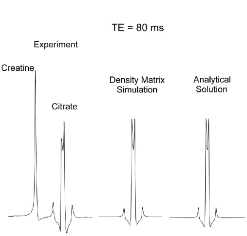
The modified PRESS was implemented on a 3T whole body MR system (Siemens, Erlangen, Germany). Localized MR spectroscopy (2x2x2 cm3 volume of interest) was performed on a phantom containing citrate and creatine; the latter metabolite was added to the solution to provide a singlet signal for amplitude and phase reference. Analytical calculations were perfomed to derive the transverse magnetization of the AB system for comparison with the experimental data and density matrix simulations [101]. Simulated free induction decays were generated for 1024 points over an acquisition time of 1 s and MR spectra were obtained by Fourier transform of the time signal. Figure 3 shows MR spectra obtained with the interpulse delays [𝑡1, 𝑡2, 𝑡3] = [20, 2, 18]𝑚𝑠. It can be noted that the inner lines of citrate are in phase
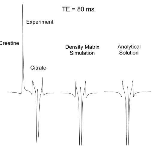
with the creatine signal. The result of the density matrix simulation is in excellent agreement with the analytical calculations and experimental data (Figure 3). With a different set of interpulse delays, [𝑡1, 𝑡2, 𝑡3] = [20, 18, 2]𝑚𝑠, keeping the same total echo time of 80 ms, a
very different MR spectrum was obtained (Figure 4) with the inner lines of citrate being in opposite phase with respect to the creatine signal.
One observation is noteworthy when comparing the spectra of Figure 3 with those of Figure
4: the signal intensity of a strongly coupled spin system has a substantial dependence on the
interpulse delays of PRESS sequences. This type of signal modulation, occurring at a constant echo time, is a unique characteristic of strongly coupled systems and could be exploited for editing purposes [90, 100]. Within the context of the density matrix formalism, the source of this signal modulation is to be found in the non-zero off-diagonal terms of the strongly coupled Hamiltonian. These elements, which are absent in weakly coupled Hamiltonians, generate a coherence mixing during the interpulse delays.
24
The density matrix simulations of MR spectra, as presented here, provide the basis for optimizing the detection of metabolites. The goal is to find the optimal sequence and sequence parameters that would yield a convenient lineshape for the metabolite of interest. Early investigations of metabolite optimization were limited to the assessment of the lineshape as a function of echo time only; it is well know that the signal intensity of weakly coupled systems is a function of the total echo time and is independent of the individual interpulse delays. However in strongly coupled systems, as we have just shown, it is necessary to simulate the MR spectra for different values of interpulse delays as well. When investigating all possible combinations of interpulse delays, the one-dimensional solution space 𝑓(𝑇𝐸) becomes a two-dimensional space 𝑓(𝑡1, 𝑡2) in the case of the standard PRESS sequence (and a
three-dimensional space 𝑓(𝑡1, 𝑡2, 𝑡3 ) in the case of the modified PRESS sequence). As a consequence, the optimization procedure would easily result into the simulation of thousands of spectra. A convenient visual representation of all these data can be achieved with the following two steps: i) calculate the signal intensity (i.e., area under the resonance signal) of each spectrum obtained with a set of parameters ([𝑡1, 𝑡2], in the standard PRESS sequence) and ii) represent the signal intensity as a function of [𝑡1, 𝑡2] in a 2D plot. How to proceed to
accomplish the first step? The direct way is to simulate the free induction decay, perform the Fourier transform to obtain the MR spectrum and then perform the signal integration to determine the area under the peak. This approach, which requires the simulation of the MR spectra for all [𝑡1, 𝑡2], is rather impractical. A different approach consists in simulating just
the first point of the free induction decay for all [𝑡1, 𝑡2]; it can be easily shown (see Appendix 2) that the area under the resonance signal is equal to the value of the first point of the free induction decay. This latter method substantially decreases the computational time of the density matrix simulations.
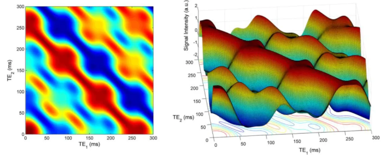
Here we show density matrix simulations (Figure 5) of the citrate signal for the standard PRESS:
90𝑥° − 𝑡
1− 180𝑦° − 𝑡1− 𝑡2− 180𝑦° − 𝑡2− 𝐴𝑐𝑞
at the field strength of 3 T. The signal intensity is plotted as a function of TE1 and TE2, where
TE1 = 2𝑡1 and TE2 = 2𝑡2. It should be noted that the signal intensity of 90000 MR spectra is
now displayed in a compact way, in Figure 5. The results of the density matrix simulations shown in Figure 5 allow us to identify the interpulse delays that maximize the signal intensity of citrate; in other words, these results allow us to optimize citrate detection.
25
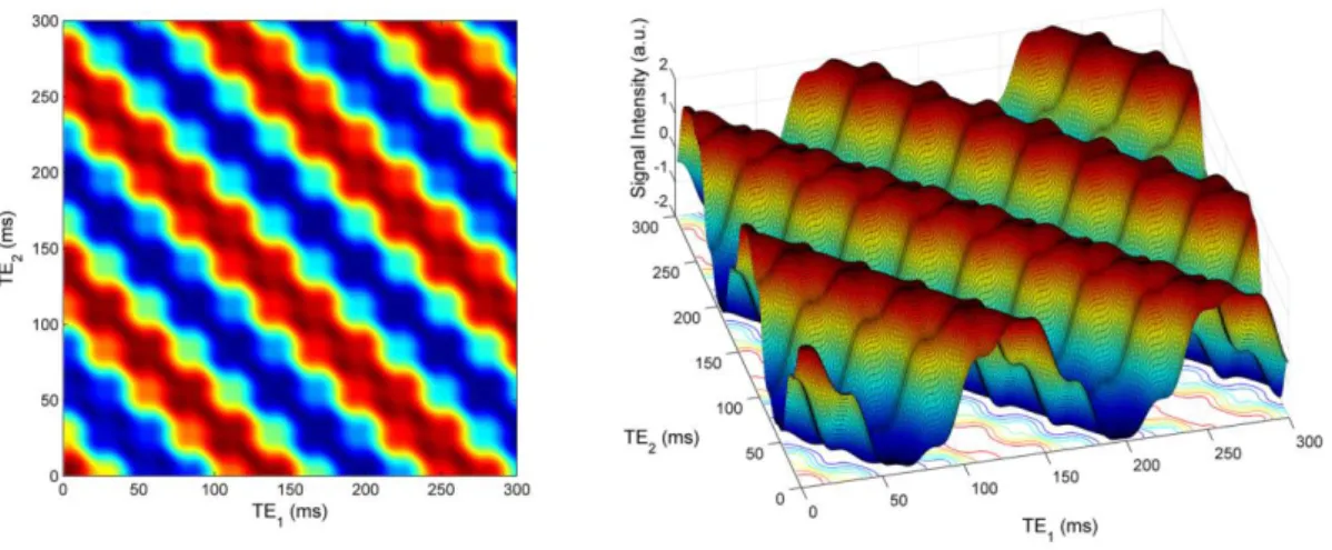
The same simulation was performed at the magnetic field of 11.7 T (Figure 6). As in Figure
5, two representations of the same data are displayed. The TE1 is on the x-axis and the TE2 is
on the y-axis. For a given TE, the points of the flat surface graph with same TE values are on the diagonal line described by the equation 𝑦 = −𝑥 + 𝑇𝐸 (that is: 𝑇𝐸2 = −𝑇𝐸1+ 𝑇𝐸). In
the case of a weakly coupled spin system, there would be no signal oscillation along these diagonal lines, that is, the "waves" would be smooth with no bumps on the crests and valleys. The signal oscillations at constant TE, to be ascribed to the coherence mixing induced by the non-diagonal elements of the Hamiltonian, show that the effects of the strong coupling in the spin system of citrate are still present at a very high magnetic field.
26
Appendix 1
Here we report the matrix representation of the angular momentum operators Ix, Iy and Iz, for
spins with quantum number ½.
Ix, Iy and Iz are the quantum mechanics analogues of the x-, y-, and z-component, respectively,
of the (classical physics) magnetization vector. These operators are the building blocks that allow for the assessment of the signal intensity by density matrix simulations.
Let’s introduce the Pauli spin matrices:
𝑔𝑥= 12(0 11 0) 𝑔𝑦 = 2𝑖(0 −11 0) 𝑔𝑧 = 12(1 00 −1)
It should be noted that the coefficient of the 𝑔𝑦 matrix is i/2, where i is the imaginary unit; on the other hand, for the 𝑔𝑥 and 𝑔𝑧 matrices the coefficient is ½.
For a single spin (spin I), the angular momentum operators Ix, Iy and Iz are represented by the
Pauli spin matrices Ix*, Iy* and Iz*, respectively:
𝐼𝑥= 𝑔𝑥
𝐼𝑦 = 𝑔𝑦 𝐼𝑧= 𝑔𝑧
Thus, the angular momentum operators for a single spin consist of 2x2 matrices.
In the case of a two-spin system (spin I and spin S), the matrix representation of the angular momentum operators needs to be modified when compared to the case of a single spin. We start with the spin I. The representation of the angular momentum operator for the spin I is obtained by the Kronecker product of Pauli matrices with the identity matrix E. We should point out that the Kronecker product of two matrices of dimensions 2x2 generates a 4x4 matrix.
The angular momentum operators Ix is given by:
𝐼𝑥 = 𝑔𝑥⊗ 𝐸
where the symbol ⊗ indicates the Kronecker product. This formula can be developed as follows:
27 𝐸 = (1 0 0 1) 𝐼𝑥 = 𝑔𝑥⊗ 𝐸 = 1 2(0 11 0) ⊗ 𝐸 = 1 2(0
∙
𝐸 1∙
𝐸 1∙
𝐸 0∙
𝐸) = 1 2( 0 ∙ 1 0 ∙ 0 0 ∙ 0 0 ∙ 1 1 ∙ 1 1 ∙ 0 1 ∙ 0 1 ∙ 1 1 ∙ 1 1 ∙ 0 1 ∙ 0 1 ∙ 1 0 ∙ 1 0 ∙ 00 ∙ 0 0 ∙ 1 ) 𝐼𝑥 = 1 2( 0 0 0 0 1 00 1 1 0 0 1 0 0 0 0 )Thus, the representation of the x-component of angular momentum operator corresponding to the spin I, for a two-spin system, is given by 4x4 matrix:
The angular momentum operators of spin S are obtained by inverting the order of the elements of the Kronecker product, that is, by taking the product of the identity matrix E with Pauli matrix:
𝑆𝑥= 𝐸 ⊗ 𝑔𝑥
Thus, the angular momentum operator SX is:
𝑆𝑥 = 𝐸 ⊗ 𝑔𝑥 = (1 0 0 1) ⊗ 𝑔𝑥 = ( 1 ∙ 𝑔𝑥 0 ∙ 𝑔𝑥 0 ∙ 𝑔𝑥 1 ∙ 𝑔𝑥) = 1 2( 1 ∙ 0 1 ∙ 1 1 ∙ 1 1 ∙ 0 0 ∙ 0 0 ∙ 10 ∙ 1 0 ∙ 0 0 ∙ 0 0 ∙ 1 0 ∙ 1 0 ∙ 0 1 ∙ 0 1 ∙ 11 ∙ 1 1 ∙ 0 ) 𝑆𝑥 =1 2( 0 1 1 0 0 00 0 0 0 0 0 0 11 0 )
Here we report the matrix representation of the angular momentum operators Ix, Iy and Iz, for
spins with quantum number ½.
The matrix representation of the y- and z-component of the angular momentum operators for the spin I and S can be obtained in the same manner, that is:
𝐼𝑦 = 𝑔𝑦⊗ 𝐸
28 and
𝐼𝑧 = 𝑔𝑧⊗ 𝐸 𝑆𝑧 = 𝐸 ⊗ 𝑔𝑧
To summarize, in the case of a two-spin system (spin I and spin S), the matrix representation of the angular momentum operators Ix, Iy and Iz and Sx, Sy and Sz is:
𝐼𝑥 =12( 0 0 0 0 1 0 0 1 1 0 0 1 0 00 0 ) 𝐼𝑦 = 2𝑖( 0 0 0 0 −1 0 0 −1 1 0 0 1 0 00 0 ) 𝐼𝑧 = 12( 1 0 0 1 0 0 0 0 1 0 0 1 −1 0 0 −1 ) 𝑆𝑥 =12( 0 1 1 0 0 00 0 0 0 0 0 0 11 0 ) 𝑆𝑦 = 2𝑖( 0 −1 1 0 0 00 0 0 0 0 0 0 −11 0 ) 𝑆𝑧 = 12( 1 0 0 −1 0 00 0 1 0 0 1 1 0 0 −1 )
The total spin angular momentum operator is then given by 𝐹𝑥 = 𝐼𝑥+ 𝑆𝑥 , 𝐹𝑦 = 𝐼𝑦 + 𝑆𝑦 and 𝐹𝑧 = 𝐼𝑧+ 𝑆𝑧 : 𝐹𝑥= 12( 0 1 1 0 1 0 0 1 1 0 0 1 0 11 0 ) 𝐹𝑦 = 2𝑖( 0 −1 1 0 −1 0 0 −1 1 0 0 1 0 −11 0 ) 𝐹𝑧 = ( 1 0 0 0 0 00 0 0 0 0 0 0 0 0 −1 )
29
Appendix 2
Here we provide the derivation of a useful formula to obtain the signal intensity, i.e., the area under the curve of the frequency-domain signal. The area under the resonance curve is by definition the integral of the frequency-domain signal 𝐹(𝜔):
𝐴 = ∫ 𝐹(𝜔)𝑑𝜔
𝜔
Using the definition of Fourier transform (𝑓(𝑡) is the time-domain signal):
𝐹(𝜔) = ∫ 𝑓(𝑡)𝑒−𝑖𝜔𝑡𝑑𝑡 𝑡
and exchanging the time and frequency integrals in the formula below we obtain: 𝐴 = ∫ ∫ 𝑓(𝑡)𝑒−𝑖𝜔𝑡𝑑𝑡𝑑𝜔 𝑡 𝜔 = ∫ ∫ 𝑓(𝑡)𝑒−𝑖𝜔𝑡𝑑𝜔𝑑𝑡 𝜔 𝑡 = ∫ 𝑓(𝑡) [∫ 𝑒−𝑖𝜔𝑡𝑑𝜔 𝜔 ] 𝑑𝑡 𝑡 .
The integral in the square brackets is the Dirac delta function, 𝛿(𝑡); inserting 𝛿(𝑡) in the equation above and using the following property of the Dirac delta function:
∫ 𝑓(𝑡)𝛿(𝑡)𝑑𝑡 = 𝑓(0)
𝑡
the formula becomes:
𝐴 = ∫ 𝑓(𝑡)𝛿(𝑡)𝑑𝑡 = 𝑓(0)
𝑡
that is, the area under the signal in the frequency domain is equal to the value of the first point of the time-domain signal.
30
Acknowledgments
My first encounter with the density matrix formalism applied to magnetic resonance spectroscopy was during my PhD thesis work. Many years have passed by and I am still indebted to my thesis director who introduced me to the wonders of the density matrix -or, as he often referred to it as, The Destiny Matrix!