HAL Id: inserm-00117223
https://www.hal.inserm.fr/inserm-00117223
Submitted on 2 Jul 2007HAL is a multi-disciplinary open access archive for the deposit and dissemination of sci-entific research documents, whether they are pub-lished or not. The documents may come from teaching and research institutions in France or abroad, or from public or private research centers.
L’archive ouverte pluridisciplinaire HAL, est destinée au dépôt et à la diffusion de documents scientifiques de niveau recherche, publiés ou non, émanant des établissements d’enseignement et de recherche français ou étrangers, des laboratoires publics ou privés.
Increased power to detect gene-environment interaction
using siblings controls.
Nadine Andrieu, Marie-Gabrielle Dondon, Alisa Goldstein
To cite this version:
Nadine Andrieu, Marie-Gabrielle Dondon, Alisa Goldstein. Increased power to detect gene-environment interaction using siblings controls.: GxE interaction and siblings controls. Annals of Epidemiology, Elsevier Masson, 2005, 15 (9), pp.705-11. �10.1016/j.annepidem.2005.01.002�. �inserm-00117223�
Increased power to detect gene-environment interaction using siblings controls
Nadine Andrieu1,2, PhD ; Marie-Gabrielle Dondon2, Msc ; Alisa M. Goldstein3, PhD
1 - Inserm EMI00-06, Tour Evry 2, 523 Place des Terrasses de l'Agora, 91034 Evry Cedex, France.
2 - Inserm IC10213 / Service de Biostatistiques, Institut Curie, 26 rue d’Ulm, 75231 Paris Cedex 5, France.
3 - Genetic Epidemiology Branch, Division of Cancer Epidemiology and Genetics, National Cancer Institute, NIH, DHHS, Bethesda, MD 20892, USA.
Address correspondence to:
EMI00-06 Inserm/ Service de Biostatistiques Institut Curie 26 rue d’Ulm 75248 Paris Cedex 05 France Tel : (33) 1 55.43.14.63 Fax : (33) 1 55.43.14.69 e-mail: [email protected] Running title:
GxE interaction and siblings controls
Acknowledgements:
This project was supported by INSERM, the US National Cancer Institute, the Foundation Philippe INC. and the Association pour la Recherche contre le Cancer (n° 9183).
HAL author manuscript inserm-00117223, version 1
HAL author manuscript
ABSTRACT
Purpose:
Interest is increasing in studying gene-environment (GxE) interaction in disease etiology. Study designs using related controls as a more appropriate control group for evaluating GxE interactions have been proposed but often assume unrealistic numbers of available relative controls. To evaluate a more realistic design, we studied the relative efficiency of a 1:0.5 case-sibling-control design compared to a classical 1:1 case-unrelated-control design and examined the effect of the analysis strategy.
Methods:
Simulations were performed to assess the efficiency of a 1:0.5 case-sibling-control design relative to a classical 1:1 case-unrelated-control design under a variety of assumptions for estimating GxE interaction. Both matched and unmatched analysis strategies were examined.
Results:
When using a matched analysis, the 1:1 case-unrelated-control design was almost always more powerful than the 1:0.5 case-sibling-control design. In contrast, when using an unmatched analysis, the 1:0.5 case-sibling-control design was almost always more powerful than the 1:1 case-unrelated-control design. The unconditional analysis of the case-sibling-control design to estimate GxE interaction, however, requires no correlation in E between siblings.
Conclusions:
Our results suggest that in most settings, a matched analysis is required and that 1:1 case-unrelated-controls design will be more powerful than a 1:0.5 case-sibling-control design.
Key words: case-control study, GxE interaction, sibling controls, study design, conditional
analysis, unconditional analysis.
INTRODUCTION
Interest is increasing in studying gene-environment (GxE) interaction in disease etiology. In general, two types of control groups are used for examining GxE interactions: unrelated (e.g. population-based) or related (e.g. sibling) controls. To date, most studies of GxE interactions have used unrelated controls. This use of unrelated controls, however, has been questioned because of the potential problem of population stratification (1-6). This potential bias from stratification was thus the motivation for some authors to propose the use of related controls as a more appropriate control group for evaluating genetic factors (7, 8). Witte et al. compared a case-control design with at least 1 control per case using population-based controls to a design using sibling (or cousin) controls. The results showed that population-based controls were most efficient for evaluating a genetic main effect, with siblings being the least efficient control group. In contrast, sibling controls were the most efficient group for detecting a GxE interaction effect. This gain in relative efficiency decreased as the frequency of the genetic factor increased (7, 8).
However, some of these evaluations may have assumed unrealistic numbers of available relative controls. For example, a review of chronic diseases like cancer have suggested that about 50% of cases may have an available sibling control (e.g. breast and stomach cancers) (9, 10)(unpublished data). Thus, in order to perform a more realistic comparison, we used simulations to compare a 1:1 case-unrelated-control study to a 1:0.5 case-sibling-control design where half of the cases have a sibling control. We also examined the effect of the analysis strategy on the efficiency of the design recognizing that for the 1:0.5 case-sibling-control design, the unconditional analysis used twice as many cases as did the conditional analysis.
METHODS
Study population
The population for the proposed studies consisted of cases and two types of controls, unrelated controls and sibling controls. We assumed that for 50% of cases it was possible to obtain an appropriate sibling control. Thus, we had a 1:1 case-unrelated-control study and a 1:0.5 case-sibling-control study. We further assumed that there was no difference in the distribution of variables of interest between cases who have sibling controls versus those cases without such sibling controls and that there was exchangeability of covariates of interest in cases and sibling controls (i.e. the covariate distribution did not depend on calendar time or
birth order or geographic location). We compared the 1:0.5 case-sibling-control design to the 1:1 case-unrelated-control study using simulations.
Table 1 shows the parameters for modeling an interaction between a genetic factor G and an environmental exposure E. G and E were assumed to be independent events. We define PE as
the prevalence of the environmental factor E in the population, PG as the prevalence of the
genetic factor G in the population. We further define the genetic factor G where the alleles at the locus are classified as A (variant) or a (wild), with population frequency p of the A allele and population frequency q for the a allele, where p+q=1. For a dominant model, AA and Aa represent subjects with G and AA represents subjects with G under a recessive model. Thus, PG=p2+2pq for a dominant model, and PG=p2 for a recessive model. Finally, we define RE as
the odds ratio between E and disease (among those not having G), RG as the odds ratio
between G and disease (among those not exposed to E) and RI as the interaction effect,
defined on a multiplicative scale.
We calculated the expected distributions of E and G in cases, matched unrelated, and matched related controls. Table 1 shows the subgroups of cases and unrelated controls at different risks for disease under a dominant genetic model and the genotype distributions of the case siblings calculated conditionally on the case genotypes. When there was a correlation in E between siblings (OREC), the probability that a case’s sibling was exposed to E was defined as in
Goldstein et al.(11) (see Appendix for details).
Simulation studies
Random numbers were generated to determine which case had a related control for each of the studies (i.e. each case had one unrelated control and approximately half of the cases had one related control).
When E and G were relatively common (e.g. both>0.05), we simulated 2500 data sets with 1000 cases:1000 matched unrelated controls:approximately 500 matched sibling controls. When E and G were relatively rare (e.g. either<0.05) (or very rare; e.g. both ≥0.01), we simulated 1000 case-control studies with 5000 (or 10,000) cases:5000 (or 10,000) unrelated controls:approximately 2500 (or 5000) sibling controls. All subjects were simulated using random numbers generated by the SAS function RANUNI (SAS, version 8, Cary, NC) to assign each of the cases and controls to the different possible E and G categories.
Analysis strategies
For the matched and unmatched analysis strategies, each simulated case-control study was analyzed by conditional and unconditional logistic regression using the program STATA (12) with a binary variable for E and a binary variable for G (based on the genotypes and inheritance model) and GxE interaction defined on a multiplicative scale.
For the unmatched strategy, we assumed that there was no correlation in E between siblings leading to the equality of the prevalences of E among unrelated controls (PEunr) and related
controls (PErel), i.e. PEunr=PErel. Thus, in such situations, an unconditional analysis may be
used to estimate the GxE interaction effect (See Appendix for further discussion).
To assess the efficiency of the 1:0.5 case-sibling-control design compared to a classical 1:1 case-unrelated-control study, we defined the relative efficiency (RE) as the ratio of the variances of βI, i.e., the variance of βI from the classical 1:1 case-unrelated-control study
divided by the variance of βI for the 1:0.5 case-sibling-control study. Variance of βI for a
given design was calculated as the average of the variances of βI from each simulated data set.
Thus, when RE>1, the 1:0.5 case-sibling-control design was more powerful than the classical 1:1 case-unrelated-control study; when RE<1, the reverse was true. We also compared RE for the unconditional analyses [RE(U)] to RE for the conditional analyses [RE(C)].
We compared RE(C) according to different frequencies of G and E (PG, PE), the main effect of
G and E (RG, RE), and the GxE interaction effect (RI). In addition, we compared the
unconditional analysis strategy to the conditional strategy for these same variables.
To evaluate the feasibility of these study designs in GxE interaction assessment, sample sizes for different scenarios were calculated using the computer program Quanto (8,13, 14) for the 1:1 case-control unconditional and the 1:0.5 case-sibling-control conditional analyses. For the 1:0.5 case-sibling-control unconditional analysis; sample sizes were approximated by the conditional 1:0.5 case-sibling-control sample sizes multiplied by ( )
( )U C RE RE . RESULTS
For completeness, we initially compared the 1:0.5 sibling-control design to a 1:0.5 case-unrelated-control design using conditional analysis for both dominant and recessive genes. Since the analysis used a conditional approach (i.e., only matched cases and controls were analyzed such that the 1:0.5 comparison was essentially a 0.5:0.5 comparison), the results for this comparison were equivalent to the comparison of a 1:1 case-sibling-control design to a
1:1 case-unrelated-control design. Therefore, as expected and previously shown by Gauderman (8), the 1:0.5 case-sibling-control design was almost always more efficient than the 1:0.5 case-unrelated-control design for both dominant and recessive models (data not shown). The gain in relative efficiency increased as RG increased and decreased as PG
increased. Variation in RE and RI had little effect on RE. When PG was very frequent (e.g.
=0.5), the relative efficiency was generally less than 1 for moderate values of RG and RI.
We also directly compared a 1:1 case-unrelated-control design to a 1:0.5 case-sibling-control design using conditional logistic regression, even though the numbers of cases and controls differed. Specifically, because of the conditional analysis approach, the 1:1 case-unrelated-control design had twice as many subjects available for the analysis compared to the 1:0.5 case-sibling-control design. Comparison of a 1:1 case-unrelated-control sample to a 1:0.5 case-sibling-control sample showed, as expected, that the 1:1 case-unrelated-control design was almost always more efficient than the 1:0.5 case-sibling-control design. The efficiency of the 1:1 case-unrelated-control design was generally 1.5 to 2 times more efficient than the 1:0.5 case-sibling-control design for reasonable parameter estimates. Only when RG was very
high (e.g. ≥10 ) (see table 2) or PG was very small, was the 1:0.5 case-sibling-control design
more efficient than the 1:1 case-unrelated-control design .
Finally, we compared a 1:1 case-unrelated-control design to a 1:0.5 case-sibling-control design using unconditional logistic regression. We assumed no correlation in E between siblings as is necessary for validity of the unconditional analyses. In general, the 1:0.5 case-sibling-control design was more efficient than the 1:1 case-unrelated-control design. Only when RG was moderate (e.g. RG=1.5) did RE decrease to less than 1. The unconditional
analysis was always more efficient than the conditional analysis (cf. table 2). RE increased more substantially for the unconditional analysis than the conditional analysis as RG, RE and
RI increased. Moreover, for numerous scenarios, the 1:0.5 case-sibling-control design which
had been less efficient than the 1:1 case-unrelated-control design under a conditional analysis strategy, became more efficient than a 1:1 case-unrelated-control design when unconditional analysis was used. For example, for a rare dominant gene with RE=1.5 or 5, RI=1.5 or 5 and
RG=3, RE<1 for conditional analysis versus RE>1 for unconditional analysis. Similar trends,
although with slightly lower RE, were observed for an equivalent recessive genetic factor (cf. table 2).
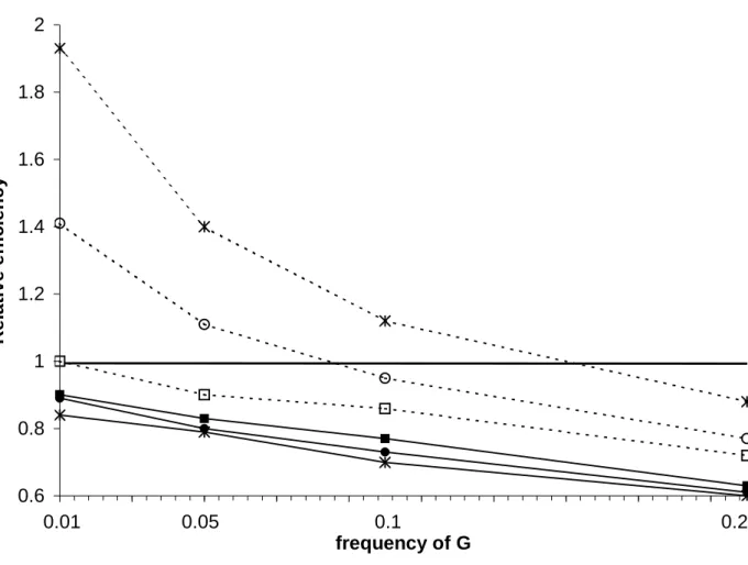
Figure 1 shows the variation of RE according to PG using conditional analyses (solid lines)
and unconditional analyses (dashed lines) for different PE values with RE=1.5, RG=3.0, and
RI=5. RE decreased as PG increased; RE also increased as PE increased with steeper slopes
observed in the unconditional analyses. As shown in figure 1, RE<1 for all conditional analysis scenarios presented; thus, the 1:1 case-unrelated-control design, with twice as many subjects involved in the analysis, was always more efficient than the 1:0.5 case-sibling-control design. In contrast, for the unconditional analysis, RE>1 when PG≤0.1 and PE>0.1.
Table 3 presents sample size (i.e. feasibility) calculations for the 1:0.5 case-sibling-control design using either unconditional or conditional analysis and for the 1:1 case-unrelated-control design using unconditional analysis. Table 3 shows that for a common gene (PG=0.2)
and moderate values of RE and RG (=1.5) (panel A) the sample sizes required to achieve 80%
power for detecting RI≥5 were similar for the 1:1 case-unrelated-control design and for the
1:0.5 case-sibling-control design analyzed using unconditional analysis. When RI decreased,
the sample sizes required increased to unrealistic numbers for all designs examined (e.g. RI=1.5; >5,700 cases and controls). For a rare gene (PG=0.001) with RE=2 and RG=5 (panel
B), for selected scenarios, neither the 1:1 unrelated-control design nor the 1:0.5 case-sibling-control design analyzed using conditional analysis reached realistic sample sizes even when RI was large (>15,000 subjects for the 1:1 case-unrelated-control design and >6,000
subjects for the 1:0.5 conditional case-sibling-control design). In contrast, for RI>5, the 1:0.5
case-sibling-control design analyzed using unconditional analysis could approach realistic sample sizes (< 3,000 subjects). Panel C shows sample size requirements for a range of different values of PG with RE=2, RG=3, and RI=5. When G was common (e.g. PG=0.2), even
though the 1:1 case-unrelated-control design was the most efficient design, the difference in required sample sizes between the traditional design and the 1:0.5 case-sibling-control design analyzed using unconditional analysis was not substantial. And when G was rare (e.g. PG≤0.01), the 1:0.5 case-sibling-control design analyzed using unconditional analysis was the
most feasible design with realistic sample sizes.
DISCUSSION
We have shown that when we used an unmatched strategy, the 1:0.5 case-sibling-control design was almost always more powerful than the 1:1 case-unrelated-control design except for weak genetic factors (RG≤1.5). In some scenarios with a common genetic factor (e.g.
PG=0.2), the sample sizes required to achieve comparable power for the 1:1
case-unrelated-control design and the 1:0.5 case-sibling-case-unrelated-control design (analyzed using unconditional analysis) were similar. Because of the sampling approach, the 1:0.5 case-sibling-control design required more cases. Therefore, if case recruitment is a limiting factor for a study, then
number of controls is the limiting factor, then the 1:0.5 case-sibling-control design may be more advantageous.
Another critical issue involves the number of available sibling controls. For this study, we assumed that 50% of cases had an available sibling control. If fewer than 50% of the cases have one available sibling control, the efficiency of the case-sibling-control design relative to the 1:1 case-unrelated-control design will decrease as the number of available siblings decreases.
The validity of the analysis for a case-sibling-control design requires a number of critical assumptions. Unfortunately, the assumptions of no difference in the distribution of variables of interest between cases who have sibling controls versus those cases without such sibling controls and exchangeability of covariates of interest in cases and sibling controls (15, 16) are not testable before the data have been collected. In addition, for validity of unconditional analyses that requires no correlation in E between siblings to estimate unbiased main environmental and/or GxE interaction effects, evaluation of the independence of E in siblings also requires completion of data collection. Conditional analysis, however, may serve as a check on the validity of the unconditional analysis strategy through evaluation of the confidence intervals for the E and GxE interaction effect estimates (RE,RI). Specifically, if the
unmatched approach is valid, given the increased efficiency for an unconditional versus a conditional analysis (partly because of the larger sample size for the unconditional analysis), the lower and upper bounds for the RE and RI confidence intervals from the unconditional
analysis should be contained within the confidence limits for the conditional analysis. If the unconditional analysis confidence interval bounds are not within the bounds for the conditional analysis, then one may expect that one or more of the required assumptions is not valid.
The unmatched approach is not valid to estimate either the G main effect or a GxG interaction effect because genotypes are not independent within sibling pairs. However, if one is interested in estimating the main effect of G or a GxG interaction effect, then the case-sibling-control design may still be used with a conditional analysis strategy.
Other study designs have been proposed to examine interaction (e.g.7, 17-24). For approaches that permit estimation of both main and interaction effects, the principle of these designs is similar to the approach that uses sibling controls, that is, increasing the frequency of the rare factors through sampling, to increase the power of the study. Among strategies that over-sampled rare factors among the control group, flexible matching strategies (20, 25) with varying proportions of an environmental matching factor among selected unrelated controls
increased the power and efficiency to detect GxE interactions in case-control studies. The highest efficiency was observed for a rare exposure that was a strong risk factor. However, this design is not recommended if the main effect of the matching factor has not been thoroughly studied or if one is interested in additive risk interactions.
Other designs have been proposed for examining main effect(s) and GxE interactions including relatives as controls (1, 7, 8, 21, 22, 24, 26). Few such designs have been evaluated for GxE interaction assessment (1, 7, 8, 24). Relative control subjects were less efficient than population-based-control subjects for detecting the genetic factor main effect, except when cases with a positive family history were over-sampled (24). However, relative control subjects were the most efficient group for detecting GxE interactions as we also observed here for either matched designs (comparison of sibling and unrelated control designs with equal numbers of cases and controls) or unmatched designs (comparison of 1:0.5 case-sibling-control to 1:1 case-unrelated-case-sibling-control designs).
Our results show that unconditional analysis of the 1:0.5 case-sibling-control design to estimate GxE interaction is unbiased under certain conditions and may produce a substantial increase in power for GxE interaction assessment. However, because of the critical assumptions required for the validity of this approach, in practice, we may find that there are few situations when unconditional analysis of a case-sibling-control study may be used. In such situations, using 1:1 case-unrelated-controls design will be more powerful than a 1:0.5 case-sibling-control design requiring a matched analytical strategy.
APPENDIX
Probability that the cases’ sibling is exposed to E
We define m as the probability that a case’s sibling is exposed to E if the case is exposed to E (P(ES=E+| EC=E+)). Similarly, we define (1-w) as the probability that a sibling has not been
exposed to E given the case has not been exposed (P(ES=E-| EC=E-)).
Given exchangeability for E, the frequency of E is the same in the case and her sibling control thus uniquely determining the joint exposure distribution between the two siblings by constraining the marginal probabilities to be equal. Thus,
(
)
E E P 1 m 1 P
w= −− . We use the following equation to define the exposure relationship between a case and his/her sibling control,
E EC E E EC P OR P 1 P OR
m= − + . When OREC=1, m=PE and there is no correlation in E between siblings
Validity of unconditional analysis using related-controls
Cases Controls related unrelated E- G- a c e G+ b d f E+ G- g i k G+ h j l
The above table shows the E and G distributions for cases, related, and unrelated controls. To be valid, unconditional analysis using related-controls should lead to unbiased estimates for the ORs of interest. Specifically, if one is primarily interested in estimating the GxE interaction effect, then only ORint needs to be unbiased. This requirement translates into the
equality of rel unr
OR
ORint = int where rel denotes related controls and unr, unrelated controls.
Thus, from the above table ORint equals
af be ak gela he ad bc ai gc ja hc OR OR OR OR OR OR unr G unr E unr G , E rel G rel E rel G , E = ⇒ = thus le kf jc id OR
ORintrel = intunr ⇒ = equation (1)
For this equality, we assume that G and E are independent i.e P(E|G)=PE . In addition, since G
is correlated in siblings, we require no correlation in E between siblings such that PErel=PEunr
which is equivalent to P(E|G)rel=P(E|G)unr, that is, i/(i+c)=k/k+e=>i/c=k/e. Then, from equation (1), we have i/c=k/e and j/d=l/f as conditions to yield rel unr
OR
ORint = int . Thus, when
there is no correlation in E between siblings, unr E rel
E OR
OR = in addition to rel unr
OR ORint = int
and an unconditional analysis can be performed in the case-related-control design to estimate the GxE interaction effect. Both the GxE interaction effect and E main effect estimates are unbiased. If, however, there is a correlation in E between siblings and/or PErel≠PEunrel, then
i/c≠k/e and j/d≠l/f. And it follows that ORrelE ≠ORunrE and rel unr
OR
ORint ≠ int . Under such
scenario(s), unconditional analysis of case-related-control data would not be valid.
Table1: Subgroups of the population at different risk of disease when there is a GxE interaction. (27)
Exposure Proportion of unrelated controls
Relative risk Proportion of cases Proportion of unaffected siblings (i.e. related controls) according to case genotypes
Case Sibling genotype
[aa] [Aa] [AA]
E+ [AA] PE p² RE RG RI (PE p² RE RG RI)/Σ*
(
)
⎟ ⎟ ⎠ ⎞ ⎜ ⎜ ⎝ ⎛ − 4 1 p 2 §(
)
⎟ ⎠ ⎞ ⎜ ⎝ ⎛ − 2 ² 1 p £(
)
⎟ ⎟ ⎠ ⎞ ⎜ ⎜ ⎝ ⎛ + 4 1 p 2 £ E+ [Aa] PE 2p(1-p) RE RG RI† (PE 2p(1-p) RE RG RI)/Σ(
)
⎟ ⎠ ⎞ ⎜ ⎝ ⎛ − + 4 2 3 p p §(
)
⎟ ⎠ ⎞ ⎜ ⎝ ⎛ − + 2 1 1 p p £(
)
⎟ ⎠ ⎞ ⎜ ⎝ ⎛ + 4 1 p p £ E+ [aa] PE (1-p)² RE PE (1-p)² RE/Σ ⎟⎟ ⎠ ⎞ ⎜⎜ ⎝ ⎛ + ⎟ ⎠ ⎞ ⎜ ⎝ ⎛ −1 1 4 p p §(
)
⎟ ⎠ ⎞ ⎜ ⎝ ⎛ − 2 2 p p £ ⎟ ⎠ ⎞ ⎜ ⎝ ⎛ 4 ² p £ E- [AA] (1-P E) p² RG (1-PE) p² RG /Σ(
)
⎟ ⎟ ⎠ ⎞ ⎜ ⎜ ⎝ ⎛ − 4 1 p 2 §(
)
⎟ ⎠ ⎞ ⎜ ⎝ ⎛ − 2 ² 1 p £(
)
⎟ ⎟ ⎠ ⎞ ⎜ ⎜ ⎝ ⎛ + 4 1 p 2 £ E- [Aa] (1-PE) 2p(1-p) RG‡ (1-PE) 2p(1-p) RG /Σ(
)
⎟ ⎠ ⎞ ⎜ ⎝ ⎛ − + 4 2 3 p p §(
)
⎟ ⎠ ⎞ ⎜ ⎝ ⎛ − + 2 1 1 p p £(
)
⎟ ⎠ ⎞ ⎜ ⎝ ⎛ + 4 1 p p £ E- [aa] (1-PE)(1-p)² 1 (1-PE)(1-p)²/Σ ⎟⎟ ⎠ ⎞ ⎜⎜ ⎝ ⎛ + ⎟ ⎠ ⎞ ⎜ ⎝ ⎛ −1 1 4 p p §(
)
⎟ ⎠ ⎞ ⎜ ⎝ ⎛ − 2 2 p p £ ⎟ ⎠ ⎞ ⎜ ⎝ ⎛ 4 ² p £ With : d=0.001 ; d d R 1 d R c E E − + = ; d d R 1 d R b G G − + = ;( )( )
( )
( )
d 1 cb R c 1 b 1 d b d 1 c R a I I − + − − − =Where a=P(D|G+,E+)=risk of disease given a person has G (G+) and E (E+); b=P(D|G+,E-)=risk of disease given a person has G+ and E-; c=P(D|G-,E+)=risk of disease given a person has G- and E+ and d=P(D|G-,E-)=risk of disease given a person does not have G or E (G-, E-)
† equal R
E under a recessive gene ‡ equal 1 under a recessive gene
* Σ=PE (p²+2p(1-p)) RE RG RI + PE (1-p)² RE + (1-PE)(p²+2p(1-p)) RG + (1-PE)(1-p)² , under dominant gene
Σ=PE p² RE RG RI + PE (2p(1-p)+ (1-p)²) RE + (1-PE)(p²) RG + (1-PE)((1-p)² +2p(1-p)), under recessive model : § multiply by (1-d)(1-P
E) when sib control not exposed to E, and by (1-c)PE when sib control exposed to E £ multiply by (1-b)(1-P
E) when sib control not exposed to E, and by (1-a)PE when sib control exposed to E
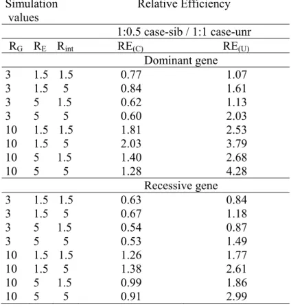
Table 2: Relative efficiency (RE) of the 1:0.5 case-sibling-control design compared to the
traditional 1:1 case-unrelated-control design using either conditional RE(C) or unconditional RE(U)
analysis for different G, E and GxE effects for a dominant or a recessive gene with PG=0.01;
PE=0.2. Simulation values Relative Efficiency 1:0.5 case-sib / 1:1 case-unr RG RE Rint RE(C) RE(U) Dominant gene 3 1.5 1.5 0.77 1.07 3 1.5 5 0.84 1.61 3 5 1.5 0.62 1.13 3 5 5 0.60 2.03 10 1.5 1.5 1.81 2.53 10 1.5 5 2.03 3.79 10 5 1.5 1.40 2.68 10 5 5 1.28 4.28 Recessive gene 3 1.5 1.5 0.63 0.84 3 1.5 5 0.67 1.18 3 5 1.5 0.54 0.87 3 5 5 0.53 1.49 10 1.5 1.5 1.26 1.77 10 1.5 5 1.38 2.61 10 5 1.5 0.99 1.86 10 5 5 0.91 2.99
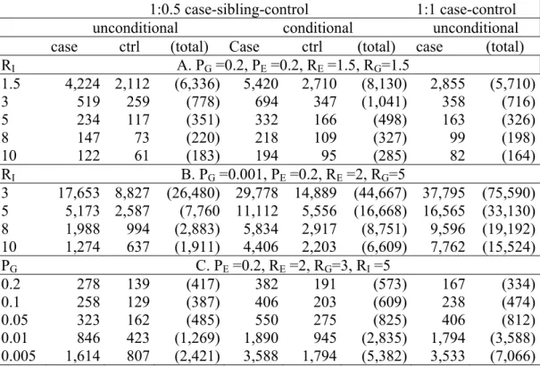
Table 3: Feasibility (i.e. sample sizes) of the 1:0.5 case-sibling-control design (using either unconditional analysis or conditional analysis) and the 1:1 case-unrelated-control design (using unconditional analysis) for a dominant gene. Numbers of cases and controls required to have 80% power to detect an interaction using a two-sided test at the 5% level are presented.
1:0.5 case-sibling-control 1:1 case-control
unconditional conditional unconditional
case ctrl (total) Case ctrl (total) case (total) RI A. PG =0.2, PE =0.2, RE =1.5, RG=1.5 1.5 4,224 2,112 (6,336) 5,420 2,710 (8,130) 2,855 (5,710) 3 519 259 (778) 694 347 (1,041) 358 (716) 5 234 117 (351) 332 166 (498) 163 (326) 8 147 73 (220) 218 109 (327) 99 (198) 10 122 61 (183) 194 95 (285) 82 (164) RI B. PG =0.001, PE =0.2, RE =2, RG=5 3 17,653 8,827 (26,480) 29,778 14,889 (44,667) 37,795 (75,590) 5 5,173 2,587 (7,760 11,112 5,556 (16,668) 16,565 (33,130) 8 1,988 994 (2,883) 5,834 2,917 (8,751) 9,596 (19,192) 10 1,274 637 (1,911) 4,406 2,203 (6,609) 7,762 (15,524) PG C. PE =0.2, RE =2, RG=3, RI =5 0.2 278 139 (417) 382 191 (573) 167 (334) 0.1 258 129 (387) 406 203 (609) 238 (474) 0.05 323 162 (485) 550 275 (825) 406 (812) 0.01 846 423 (1,269) 1,890 945 (2,835) 1,794 (3,588) 0.005 1,614 807 (2,421) 3,588 1,794 (5,382) 3,533 (7,066)
0.6 0.8 1 1.2 1.4 1.6 1.8 2 frequency of G Relative efficiency 0.01 0.05 0.1 0.2
Figure 1: Relative efficiency (RE) according to the frequency of G for a dominant gene and for different values of PE with RI=5,
RE=1.5, RG=3. RE is defined as the ratio of the variance of βI of the classical 1:1 case-control study design divided by the variance of
βI of the 1:05 case-sibling-control design using either conditional analysis (solid lines) or unconditional analysis (dashed lines).
(P =0.5: starred-solid and -dashed lines; P =0.1: circled-solid and -dashed lines; P =0.01: squared-solid and -dashed lines)
16
References
1. Gauderman WJ, Witte JS, Thomas DC. Family-based association studies. J.Natl.Cancer Inst.Monogr 1999;31-7.
2. Wacholder S, Rothman N, Caporaso N. Counterpoint: bias from population stratification is not a major threat to the validity of conclusions from epidemiological studies of common polymorphisms and cancer. Cancer Epidemiol.Biomarkers Prev. 2002;11:513-20.
3. Thomas DC, Witte JS. Point: population stratification: a problem for case-control studies of candidate-gene associations? Cancer Epidemiol.Biomarkers Prev. 2002;11:505-12. 4. Freedman ML et al. Assessing the impact of population stratification on genetic
association studies. Nat.Genet. 2004;36:388-93.
5. Caporaso N, Rothman N, Wacholder S. Case-control studies of common alleles and environmental factors. J.Natl.Cancer Inst.Monogr 1999;25-30.
6. Millikan RC. Re: Population stratification in epidemiologic studies of common genetic variants and cancer: quantification of bias. J.Natl.Cancer Inst. 2001;93:156-8.
7. Witte JS, Gauderman WJ, Thomas DC. Asymptotic bias and efficiency in case-control studies of candidate genes and gene-environment interactions: basic family designs. Am.J.Epidemiol. 1999;149:693-705.
8. Gauderman WJ. Sample size requirements for matched case-control studies of gene-environment interaction. Stat.Med. 2002; 21[1], 35-50.
9. Andrieu N, Demenais F. Interactions between genetic and reproductive factors in breast cancer risk in a French family sample. Am.J.Hum.Genet. 1997;61:678-90.
10. Botto LD, Khoury MJ. Commentary: facing the challenge of gene-environment interaction: the two-by-four table and beyond. Am.J.Epidemiol. 2001;153:1016-20.
11. Goldstein AM, Hodge SE, Haile RW. Selection bias in case-control studies using relatives as the controls. Int.J.Epidemiol. 1989;18:985-9.
12. Stata Corp. Stata statistical software: Release 7.0. College station, Tx: Stata corporation. 2001.
13. Gauderman WJ. Sample size requirements for association studies of gene-gene interaction. Am J Epidemiol 2002, 155:478-84.
14. Gauderman WJ. Candidate gene association studies for a quantitative trait, using parent-offspring trios. Genet Epidemiol 2003, 25:327:38.
15. Langholz B et al. Ascertainment bias in rate ratio estimation from case-sibling control studies of variable age-at-onset diseases. Biometrics 1999;55:1129-36.
16. Siegmund KD, Langholz B. Ascertainment bias in family-based case-control studies. Am.J.Epidemiol. 2002;155:875-80.
17. Langholz B, Clayton D. Sampling strategies in nested case-control studies. Environ.Health Perspect. 1994;102 Suppl 8:47-51.
18. Breslow NE. Case-control study, two phase. New York, NY: Wiley, 1998.
19. Sturmer T, Brenner H. Potential gain in efficiency and power to detect gene-environment interactions by matching in case-control studies. Genet.Epidemiol. 2000;18:63-80.
20. Sturmer T, Brenner H. Flexible matching strategies to increase power and efficiency to detect and estimate gene-environment interactions in case-control studies. Am.J.Epidemiol. 2002;155[7], 593-602.
21. Weinberg CR, Umbach DM. choosing a retrospective design to asses joint genetic and environmental contributions to risk. Am.J.Epidemiol. 2000;152[3], 197-203.
22. Umbach DM, Weinberg CR. The use of case-parent triads to study joint effects of genotype and exposure. Am.J.Hum.Genet. 2000;66[1], 251-261.
23. White JE. A two stage design for the study of the relationship between a rare exposure and a rare disease. Am.J.Epidemiol. 1982;115, 119-128.
24. Siegmund KD, Langholz B. Stratified case sampling and the use of family controls. Genet.Epidemiol. 2001;20, 316-327.
25. Saunders CL, Barrett JH. Flexible matching in case-control studies of gene-environment interactions. Am.J.Epidemiol. 2004;159:17-22.
26. Schaid DJ. Case-parents design for gene-environment interaction. Genet.Epidemiol. 1999; 16[3], 261-273.
27. Andrieu N, Goldstein A. The case-combined-control design was efficient in detecting gene-environment interactions. J.Clin.Epidemiol. 2004; 57: 662–71