HAL Id: hal-02071770
https://hal.archives-ouvertes.fr/hal-02071770
Submitted on 12 Aug 2019HAL is a multi-disciplinary open access
archive for the deposit and dissemination of sci-entific research documents, whether they are pub-lished or not. The documents may come from teaching and research institutions in France or abroad, or from public or private research centers.
L’archive ouverte pluridisciplinaire HAL, est destinée au dépôt et à la diffusion de documents scientifiques de niveau recherche, publiés ou non, émanant des établissements d’enseignement et de recherche français ou étrangers, des laboratoires publics ou privés.
The Power to Create Chaos
Konrad Hinsen
To cite this version:
Konrad Hinsen. The Power to Create Chaos. Computing in Science and Engineering, Institute of Electrical and Electronics Engineers, 2016, 18 (4), pp.75-79. �10.1109/MCSE.2016.67�. �hal-02071770�
The power to create chaos
Konrad Hinsen
Occasionally I receive feedback from readers on the articles I write for the Scientific Programming department. My recent article on technical debt [1] pro-voked more feedback than anything else I have written here before, so I suspect the topic resonated with many readers. Most the e-mails I received were about personal experiences people had with technical debt that was recognized too late to be handled gracefully. But a few concentrated on a very specific point: my claim that computers exhibit chaotic behavior, and that this is a problem when using them in research. I will take those reactions as a pretext to elaborate a bit on that point, which is in my opinion not yet sufficiently appreciated.
I call this a pretext because I won’t actually address the objections that were raised in much detail. They focused on the problems of defining chaos mathemat-ically for discrete rather than continuous systems. The standard definitions of chaos refer to infinitesimal changes in the initial conditions, which for computers and other discrete state systems make no sense, because the smallest possible change is one bit. Readers interested in this topic can find detailed discussions in the literature on cellular automata, for which Stephen Wolfram’s “A New Kind of Science” [2] is a good entry point, in particular chapters 4 and 7. However, in the context of scientific programming, which is the topic of this department, the precise mathematical definition of chaotic behavior is much less relevant than its consequences on software development and testing.
Chaos is a mathematical concept from the theory of dynamical systems. A dynamical system is defined by a state space and a time evolution rule for the state. The system starts in some initial state, and then the time evolution rule is applied to yield subsequent states. Both the state space and the time variable can be continuous or discrete. A computer is a dynamical system with a discrete state, which consists of the computer’s memory and its processor’s internal state. Time is discrete as well, the elementary time step being the execution of one pro-cessor instruction. The propro-cessor’s instruction set provides the details of the time evolution rule. The initial conditions of a computation are the memory contents plus processor state when the computation is started. Execution proceeds until the program reaches its end – if it ever does. The final memory contents contain the result of the computation. Note that “memory” should be understood in a wide enough sense to include all data storage available, including hard disks, network storage, etc. Note also that what I consider here is computation in the
narrow sense of mechanically processing information. When you add multiple processes, communication between them, or external events, everything becomes more complicated.
The defining aspect of chaos is a strong sensitivity of a dynamical system’s behavior on initial conditions: small changes in these conditions can cause large changes in the system’s future behavior for which no useful bounds can be es-tablished. Chaotic behavior in nature makes the long-term evolution of many phenomena unpredictable even though they are deterministic. An often cited ex-ample is the weather, which can be predicted for only a very short time – about a week – not because of any inherently random processes, nor because a lack of computational power, but because the initial conditions that enter into the prediction can be measured only to some finite precision.
Computers are engineered dynamical systems for which such problems do not exist. We know the initial state of a computation precisely, and we can even store it for future re-use. But changes in the initial state are of interest as a way to explore the consequences of errors. Erratic behavior of the computing hardware itself is rare enough that it can safely be ignored, except for the extremely large parallel computers. But human errors in the preparation of the initial state – the program and the input data – are an important cause of wrong results. That’s why it makes sense to ask the question how the behavior of a computation changes if the correct initial state is modified in some way.
Saying that a computer behaves chaotically means that the result of a com-putation depends strongly on the initial state, to the point that a small change in this initial state can change the result beyond any useful predictable bound. As I already mentioned, some of the criteria of traditional chaos theory do not apply: changes cannot be made infinitely small, as the smallest possible change is a one-bit flip, and deviations cannot become infinite, because the computation’s state consists of a finite number of bits. The latter restriction applies to every physical system, of course, but the finiteness of the our planet’s atmosphere has not prevented scientists from applying chaos theory to weather forecasting.
The mechanism that causes chaotic behavior in computation is the amplifi-cation of small changes by subsequent steps. The impact of a one-bit flip can be small, for example if the bit happens to represent the least significant digit of an input number. At the other extreme, a one-bit flip in a processor instruction can crash the program, leading to no useful result at all. In between these two extremes, a one-bit flip can lead to results that differ from the correct result in arbitrary ways. The worst case is not a program crash, nor a huge difference in the final result, but a wrong result that looks credible. Such a mistake has a good chance of going unnoticed.
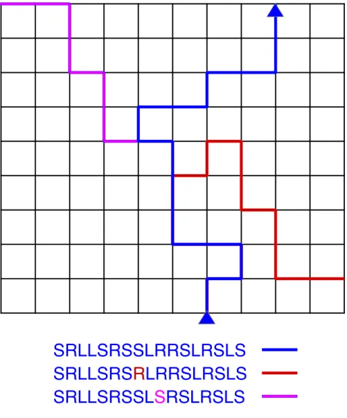
I found a nice simple illustration for error amplification in computation in a lecture by G´erard Berry [3]. Suppose you live in a city with a grid-like street layout (see Figure 1). You want to explain to a friend at the other end of the city how to reach you by car. You provide a list of driving directions that tell
your friend at every corner what to do: turn left (L), turn right (R), or continue straight on (S). Your driving instructions are thus a string made of the letters L, R, and S, which is not very different from a program written as a list of processor instructions. By following these instructions, your friend will move along the blue path from the bottom of the grid to the top.
But now suppose that some mistake happens in transmitting the driving direc-tions, or that your friend takes a wrong turn while driving. The smallest possible mistake would be the replacement of a single letter. Two such minimally modi-fied instruction sequences are shown in Fig 1, in red and violet, together with the resulting paths. It is clear that the places one reaches by following these modified instructions are not at all close to the real destination, nor close to each other. In fact, minimal mistakes can take you anywhere on the grid.
In this simple example, the mechanism of error amplification is easy to un-derstand. Each minimal one-letter change rotates the remaining part of the path by 90 degrees compared to the correct one. The more steps remain to be done after the mutated instruction, the farther the arrival point will be from the in-tended one. That is also the general mechanism that makes the outcome of a computation in the presence of mistakes so hard to predict.
An error that grows linearly with the number of computational steps isn’t really that bad. It doesn’t yet deserve the label “chaotic behavior”. After all, our “driving directions” programming language provides several useful guarantees. No matter what mistake you make, a “program” consisting of N instructions is guaranteed to terminate after exactly N steps and yield a valid position on the grid (assuming the grid is big enough), which moreover is at most 2N grid steps away from the intended destination. There is no possibility of non-termination (driving around the grid endlessly) or a crash (hitting an invalid position). We don’t get such guarantees for the programs we use in computational science. The reason why we do get them for our driving directions is that the language is very limited. It can be processed by what is known as a “finite state machine” in automata theory, whereas standard programming languages require a more powerful automaton – in fact, the most powerful type of automaton that is known today – called a “Turing machine”. As in other aspects of life, more power also means more responsibility, as mistakes can have more serious consequences. Turing machines give you so much power that you can easily create chaos (see e.g. [4]). If we added features such as loops or tests based on the current position to our driving directions language, we would need a Turing machine for processing it. That would give us the power to condemn our friends, intentionally or by mistake, to spend the rest of their lives driving around the city.
In writing scientific software using Turing-complete languages, we have ex-actly that power and we should be constantly watching out for unexpected con-sequences of mistakes. However, that is not how computational scientists behave in practice. The dominant attitude is to trust computational results if they “look right”, i.e. if they are not in disagreement with expectations and prior
knowl-edge of the problem under study. I have even heard people say that they “trust their intuition” to spot potential mistakes in the results. That is not in itself an absurd idea. Experienced experimentalists do recognize suspect results coming from instruments they know well. It is certainly possible to develop an intuition for the credibility of data.
The crucial difference is that experimental equipment is carefully designed not to exhibit chaotic behavior, such that minor damage or production defects do not lead to unexpected results. If you put a mite under a microscope, a defect in the instrument may lead to a blurred image, but not to an image showing an extra pair of legs. If the image is sharp enough to let you count the legs of the mite, then you know you can trust that observation. But this approach doesn’t carry over to software. There is no typical symptom of a programming mistake – anything is possible. Even the most experienced software developers can’t judge if a program is correct by inspecting the source code, or by running it on a few sample inputs, except if the program is trivially small. Moreover, in many applications of computational science, correctness of a program isn’t even something one could aim for. We can only decide if a program is correct if we have some other means of specifying what the correct result is. This is often not the case in a research setting, where much code is written for computing quantities that nobody has ever computed before.
A common attitude that we should probably start to question in this context is the one of considering computation as mechanized mathematics. The focus of mathematics is on precise statements that can be proven right or wrong. In research, we often use computation for exploring imprecise statements – scientific hypotheses – whose domains of validity are not known yet. A useful complemen-tary notion to mathematical correctness is the robustness of the computational tools we use. This is well explained in an essay by Gerald Sussman that draws on his background in electrical engineering [5]. A robust computer program produces reasonable output for reasonable input, even if the latter is different from what the program was initially designed to handle. We have similar concepts in com-putational science, for example the notion of numerical stability of algorithms. But robustness criteria do not play a major role in the design and implementation of scientific software today.
In order to link these abstract considerations of potential chaotic behavior to the practice of computational science, I tried to apply them to my own work in molecular simulations. Most of my work is about extracting information from simulation trajectories, which are datasets about 1 GB in size – too big for inspec-tion by eye, but small enough to be processed on my laptop. I spend much of my day writing, modifying, and running Python scripts that perform various geomet-rical and statistical analyses on these trajectories. These scripts are rather short, but rely on a collection of libraries, ranging from general and widely used ones such as NumPy (http://www.numpy.org/) or h5py (http://www.h5py.org/)) to
domain-specific ones such as MOSAIC (http://github.com/mosaic-data-model/mosaic-python).
The computation that is performed when I run one of my scripts is defined by the script, the file containing the trajectory, the Python language, and all the libraries used by the script. But that’s just the immediately visible part. The libraries I have cited depend on other libraries, and the Python interpreter is written in C. A different way to present this complex assembly of software is as a set of consecutive layers that transform a general-purpose computer into a tool for performing a very specific analysis of a simulation trajectory. Each of these layers can be described in terms of (1) the notation in which the additional information being added is expressed, and (2) the tool that processes this information:
1. The processor instruction set, executed by the computer.
2. The C language, translated into processor instructions by a C compiler.
3. The Python language, executed by an interpreter written in C.
4. The Python language augmented by the NumPy library, written in C and plain Python.
5. ... more libraries ...
6. The file format for the data files, interpreted by an analysis script written in Python augmented by various libraries.
All the layers listed above define both a part of the computation and the notation in which some other part of the computation is expressed. For example, the Python language defines the data representation and memory management aspects of the computation, in addition to defining what is and is not a legal Python program. My analysis script defines all the algorithms, but also the input file format for the trajectories.
For historical and practical reasons, we use different labels to refer to these notations: the first three are called “programming languages”, whereas the last one is a “file format”. The intermediate ones that simply add libraries are rarely recognized as distinct notations at all. To see that they really are, consider the small Python script
import numpy
print(numpy.arange(5))
This is not a valid program in the Python language, but it is a valid program in the Python-plus-NumPy language, which shows that these two languages are distinct. Libraries should thus be treated as language extensions.
All the layers but the last one are general-purpose Turing-complete program-ming languages. There are of course significant differences between them, which is
why these different layers exist. The processor instruction level is not very conve-nient for human programmers, being difficult to read and understand. Moreover, processor instructions are a high-risk notation: any sequence of bytes can be ex-ecuted as instructions, but most byte sequences will not produce anything useful and may even cause damage to data stored in the computer. The C language is much more convenient, and also provides a better level of verification, because many possible mistakes are caught by the compiler. The Python language is even more convenient, and helps to avoid mistakes by expressing a computation in much fewer lines of code. Similarly, each library layer adds more convenience for computations made up of the kind of operations that these libraries imple-ment, and at the same time prevents mistakes by allowing the programmer to write less code for a specific computation.
However, none of these layers adds useful guarantees about the behavior of the computation. The potential of generating chaos remains present until the very last layer, which is defined by my trajectory analysis script. From the point of view of robustness, it would be preferable to have as much of the computation as possible expressed using notations that limit the impact of mistakes. Instead of libraries that add optional shorthand notation for some operations to a general-purpose language, we should have successive layers of languages that enforce the use of a more specialized and less dangerous notation.
This idea is sometimes advocated as the “principle of least power” [6]: every aspect of a computation should be described in a language with just as much expressive power as strictly required for the task. The additional guarantees that a limited language can make also offer more opportunities for analyzing and optimizing a program. Many Domain-Specific Languages (DSLs) are based on this idea. I have written about DSLs before in this department [7]. In contrast to a library, a DSL is both more and less than a general-purpose language. The “less” part often includes giving up Turing-completeness. A data file format is then nothing but an extreme case of a DSL, in which only constant data is allowed and no algorithm can be expressed at all.
The main obstacle to such an approach is probably psychological. We asso-ciate the term “language” in the context of programming with something complex that takes many years to master. Most computational scientists would be happy to get away with learning only one programming language in their life. But as I explained above, a language can be a small variation on another one. Just as today’s libraries are extensions to general-purpose languages, we could have library-like pieces of code that remove or restrict features of languages. As an example, removing while-loops and recursive function calls would turn Python into a language in which every program is guaranteed to terminate. A quick inspection of the trajectory analysis scripts that I wrote over the last few months showed that they could all be written in such a restricted Python dialect. In fact, they already are. I rarely need all the power that Python gives me. But I cannot ask Python to verify that I didn’t use that power by mistake.
These observations apply with minor variations in languages, libraries, and file formats to most computations done today in science and engineering. In the short history of computing, we can observe a general tendency towards providing more expressive power wherever some aspect of a computation is defined. In the early days, we had Fortran programs reading simply structured input files. But as soon as computers could handle larger programs, embedded scripting languages – usually Turing-complete – became a desirable feature for customizing application software. From there it was a small step to writing application software in a scripting language augmented by domain-specific libraries, as illustrated by my above example. There are even cases of languages that became accidentally Turing-complete as features were added, the best-known example being C++ templates. It is in fact possible to do arbitrary computations, including chaotic ones, as part of the compilation of a C++ program. The downsides of too much freedom in program structure have been known for a while, and have lead to the widespread adoption of structured programming in the 1980s and to the growing popularity of functional programming in recent years [8]. But advocates of these approaches to safer programming were always keen to point out that no expressive power is lost in adopting them. Perhaps it is time to re-evaluate the importance of computational omnipotence.
Konrad Hinsen is a researcher at the Centre de Biophysique Mol´eculaire in Orl´eans (France) and at the Synchrotron Soleil in Saint Aubin (France). His re-search interests include protein structure and dynamics and scientific computing. He has a PhD in theoretical physics from RWTH Aachen University (Germany). Contact him at [email protected].
References
[1] Konrad Hinsen
”Technical Debt in Computational Science”
Computing in Science and Engineering 17(6), 103–106 (2015)
[2] Stephen Wolfram
”A new kind of science”
Wolfram Media, Champaign, IL, 2002, http://www.wolframscience.com/
[3] G´erard Berry
”Pourquoi et comment le monde devient num´erique” Le¸con inaugurale 2007-2008, Coll`ege de France
http://www.college-de-france.fr/site/gerard-berry/ inaugural-lecture-2008-01-17-18h00.htm
[4] Nabarun Mondal, Partha P. Ghosh
”Universal Computation is ‘Almost Surely’ Chaotic”
SOP Transactions on Applied Mathematics , in press (2015) http://www.scipublish.com/journals/AM/papers/1506
[5] Gerald Jay Sussman
”Building Robust Systems”
http://groups.csail.mit.edu/mac/users/gjs/6.945/readings/ robust-systems.pdf [6] Tim Berners-Lee ”Principles of Design” http://www.w3.org/DesignIssues/Principles.html [7] Konrad Hinsen
”A glimpse of the future of scientific programming”
Computing in Science and Engineering 15(1), 84-88 (2013)
[8] Konrad Hinsen
”The promises of functional programming”