Design of a fluid elastic actuator with application to structural control

(1)

DESIGN OF A FLUID ELASTIC

ACTUATOR WITH APPLICATION TO

STRUCTURAL CONTROL

Mark K. Ciero, Lt. U.S.A.F.

B.S., Aeronautical Engineering B.S., Engineering Mechanics United States Air Force Academy, 1991

Submitted to the Department of Aeronautics and Astronautics in Partial Fulfillment of the Requirements for the Degree of

MASTER OF SCIENCE in AERONAUTICS AND ASTRONAUTICS at the

MASSACHUSETTS INSTITUTE OF TECHNOLOGY

May 1993

Signature of Author

Department of Aeronautics and Astronautics May 7, 1993 Certified by

Professor Hugh L. McManus Department of Aeronautics and Astronautics Thesis Advisor Accepted by

S, " -Professor r2 Y. Wachman Chairminh, Department Graduate Committee

Aero

MASSACHUSETTS INSTITUTE

OF TFfIfI11 nY

'JUN

08 1993

LibhMIZOc

(2)

DESIGN OF A FLUID ELASTIC

ACTUATOR WITH APPLICATION TO

STRUCTURAL CONTROL

by

MARK K. CIERO, Lt. U.S.A.F.

Submitted to the Department of Aeronautics and Astronautics on

May 7, 1993 in partial fulfillment of the requirements for the Degree of Master of Science in Aeronautics and Astronautics

ABSTRACT

An elastically deformable pressure vessel is used as an actuator. The internal pressure is controlled hydraulically via force applied to an external bellows. The resulting elongation of the vessel is a linear function of the input force, and depends on the physical properties of the vessel, fluid, and bellows. The design includes an orifice through which fluid flows, adding damping to the actuator.

Mathematical models of the actuator are developed which relate performance of the actuator to its geometry and material properties. A

static analysis yields the linear relationship between the commanded input force and the resulting elongation of the vessel. A model of the passive (no input force) response of the actuator indicates it will act as a passive

damper. The active response (application of a dynamic input force yielding a dynamic elongation) is limited in frequency by the orifice damping.

Strategies for optimizing the actuator size and material properties are developed from the models.

Actuators manufactured with differing materials and fluids were tested. The static results are linear and matched the analysis. The passive results and the model predictions confirm that the configuration of the actuators, as built, is poor for passive damping. The correlation between the model and active experiments is excellent. Actuation bandwidth is

shown to be selectable by selecting orifice size. Tailoring the material properties of the vessel by the use of optimally designed composite laminates results in a factor of two improvement in the performance.

The actuator is useful for structural control. It's performance is comparable to other available actuators, it is constructed of off-the-shelf hardware, and it has the advantages of a built-in frequency limit and easily

customizable performance characteristics. Thesis Advisor: Professor Hugh L. McManus Title: Boeing Assistant Professor

(3)

Acknowledgement

In the short two years that I have been here (which recently have seemed like two decades), I have had the privelege of meeting and working with so many brillant good-natured people.

The top of the list begins with my advisor, Professor Hugh McManus. Without his guidance, his time, and a couple of cups of coffee (that he

bought), this thesis would not be possible. His insight and ability to solve problems were a charachteristic that I admired (and hoped a little has rubbed off on me). I am very grateful. Thank you.

To everyone at the Space Engineering Center whom I have gotten to know and joked with thanks for keeping me sane. The help of so many of you was much appreciated. I certanly will miss the lab. (I think, thanks to the Air Force, I will reach orbital velocity the first time out.)

To Professor Jack Kerrebrock, thank you for the concept and for recruiting me. I hope this thesis represents just the first tidbit of what is possible with your idea.

To my wife, who married me knowing the thesis was on the horizon but, probably, did not anticipate the role of late-night editor, thank you. If it had not been for you my organization may have drowned me. I consider myself extremely fortunate to have found a person as understanding and willing to help as you. You have demonstrated so clearly that our friendship and companionship, no matter what the future entails, is a constant that we can trust in. Thank you.

This research was funded by the Space Engineering Research Center (SERC) at the Massachusetts Institute of Technology. I am grateful to have had the opportunity to work on this project.

I also appreciate the support of the Air Force Institute of Technology, Wright Patterson Air Force Base, Ohio.

(4)

List of Figures

1.1 P-Strut Concept: An Elastic, Axially Deformable Body

Under Internal Fluid Pressure... 17

1.2 Static, Active, and Passive Modes of Operation... 17

2.1 An Overview of the Controlled Structures Field ... 23

2.2 1-DOF M odel... ... 26

2.3 Bode Diagram of 1-DOF Model ... 26

2.4 A Control System Diagram... 28

2.5 Passively Damped System Model... 29

2.6 System Actuator Model ... ... 32

3.1 Description of the P-Strut Geometry... 39

3.2 P-Strut Bellows and Orifice Geometry... 41

3.3 Definition of Longitudinal (1) and Hoop (2) Coordinate Directions ... ... 41

3.4 Typical Composite Laminate Layup... 44

3.5 Pressurized Circular Cylinder... 47

3.6 P-Strut Radial Swelling and End Effects... . 50

3.7 Pressurized Isotropic Circular Cylinder End Effects ... 50

3.8 Longitudinal and Radial Volume Changes ... 53

3.9 Total Volume Change and Input Stroke... . 53

3.10 A Circular Orifice with Viscous Fluid Flow and the Mechanical Dashpot Representation ... 60

3.11 P-Strut Schematic in Passive Mode of Operation ... 65

3.12 Passive Discrete Stiffness Model ... 70

3.13 Passive Performance (Kp,,,) Bode Diagrams: Magnitude and Phase Versus Frequency... ... 73

3.14 A Schematic of the D-Strut ... ... 78

3.15 Revised Passive Discrete Stiffness Model ... 81

3.16 Revised Passive Performance Bode Plots ... 81

3.17 P-Strut Schematic in Active Mode of Operation ... 83

3.18 Discrete Active Performance (Admittance) Model ... 88

3.19 Active Performance Admittance (A, t) Bode Diagrams: Magnitude and Phase Versus Frequency... 88

(8)

4.1 P-Strut Vessel Radius Versus Input Force... 93

4.2 P-Strut Vessel Length Versus Input Force... 93

4.3 Poisson's "Scissoring" Effect: TF Versus Composite Four Ply Layups... 97

4.4 P-Strut Side View ... 100

4.5 P-Strut Axial View ... 101

4.6 P-Strut Top View ... 101

4.7 Solenoid-Bellows-Orifice Connections...102

4.8 An "Optimal" Vessel for the P-Strut Design ... ... 04

5.1 Chemical Milling Sample Test Results ... 107

5.2 Overlap of Composite Plies During Layup Cross-Sectional View...109

5.3 Axial Cross-Section: P-Strut Cure Preparation ... 109

5.4 Bleed/Fill Diagram ... 111

5.5 P-Strut Instrum entation...113

5.6 View of Component Tester...113

6.1 Longitudinal Strain vs. Hoop Strain ... 121

6.2 Hoop Strain vs. Input Force...121

6.3 Pressure vs. Input Force ... 122

6.4 Input Stroke vs. Input Force...122

6.5 Isotropic Performance: Elongation vs. Input Force...123

6.6 Isotropic Performance: Elongation vs. Input Stroke...123

6.7 Hybrid Performance with 10K cs Silicon Fluid: Elongation vs. Input Force ... 124

6.8 Hybrid Performance with 10K cs Silicon Fluid: Elongation vs. Input Stroke ... 124

6.9 Hybrid Performance with 30K cs Silicon Fluid: Elongation vs. Input Force ... 125

6.10 Hybrid Performance with 30K cs Silicon Fluid: Elongation vs. Input Stroke ... 125

6.11 Hybrid Performance with Glycerol Fluid: Elongation vs. Input Force ... ... 126

6.12 Hybrid Performance with Glycerol Fluid: Elongation vs. Input Stroke ... 126

6.13 Composite Performance: Elongation vs. Input Force ... 127

6.14 Composite Performance: Elongation vs. Input Stroke ... 127

(9)

6.16 Hybrid Passive Performance... ... 131

6.17 Hybrid Passive Performance with No Fluid ... 132

6.18 Composite Passive Performance ... ... 132

6.19 Isotropic Active Performance ... 136

6.20 Hybrid Active Performance with 30K cs Silicon and Glycerol Fluids ... 136

6.21 Composite Active Performance with Increasing Orifice Sizes (30, 40, 55, 70, 82 m il) ... 137

6.22 Composite Active Performance ... 137

A.1 Pressurized Isotropic Circular Cylinder ...151

A.2 Hoop and Longitudinal Strain in an Isotropic Cylinder ... 153

(10)

List of Tables

3.1 Passive Frequency Characteristics... 72

3.2 A Parameteric Study of the Passive Performance Model ... 76

3.3 A Parameteric Study of the Active Performance Model ... 90

4.1 A Comparison of the Numbers of Composite Wraps Versus The Static Performance of a Hybrid Aluminum-Composite ... 95

4.2 A Comparison of P-Strut Composite Layups Versus the Static Performance... 96

4.3 Properties of the P-Strut's Viscous Fluids ... 98

4.4 The Dimensions of the Three P-Strut Designs ... 103

5.1 Instrumentation List and Characteristics... ... 114

6.1 Static Performance Results: ... 128

6.2 Constants Used in Correlation of Static Performance Results...128

6.3 Measured Passive Performance ... 133

6.4 Epoxy Parameters Fit to Passive Data ... 133

(11)

Nomenclature

C,, KAS,N, Y, e, r b v,G SE22 _E _l 12L ₂ 2L_1.9G1, G1 A,X,Bd A Aact ADCact AzC AC Ab

Ao

B, B

State Space System Matrices

Composite Thickness Weighted Stiffness Matrix Admittance of P-Strut in Active Model

Admittance at DC Frequency

Area of Cylinder Wall (i.e. Annulus Area) Cross-Sectional Area of Cylinder

Effective Cross-Sectional Area of Bellows Cross-Sectional Area of Orifice

Bulk Modulus of the Fluid Bandwidth (Frequency)

Damping Coefficient Multiplied by Area Ratio Control State Space Matrices

Damping Coefficient

Damping of Structure or Orifice Modeled Damping Coefficient

Damping Coefficient Used in Passive Model Laminar Flow Damping or Dashpot Coefficient Turbulent Flow Damping or Dashpot Coefficient Laminate Compliance Matrix

Diameter of Orifice

Material Property Matrix

Isotropic Material Properties (Young's

Modulus, Poisson's Ratio, Shear Modulus) Laminate Effective Direction Material Properties Input Force into Bellows

Disturbance Force from Structure into Actuator Force from Actuator into Structure

Laminar and Turbulent Head Loss Coefficients Head Loss Coefficient Due to Roughness or Blunt

Orifice Ends Structural Stiffness C,, C C, Clam C tur CL Do E

E,

EllL Fb Fd FL hlam,hturb hend

(12)

K

kb

K,

KL Kpass gpas8 r KR

Ks

KDCp

KDCep, Kep,Cep K,-L, Leff Ldev

Lo

M P Pb Ri, Re, Ro Re s t tealr, comp tdev t dev tr V0 Z

Stiffnesses Associated with the Passive Damping Model

Static Stiffness of Bellows

Static Stiffness of Bellows Multiplied by Area Ratio Volumetric Stiffness of Fluid

Longitudinal Stiffness

Complex Stiffness of P-Strut in Passive Model Revised Complex Stiffness of Passive Model Hoop or Radial Dilation Stiffness

Structural Stiffness of Bellows Passive Stiffness at DC Frequency

Epoxy Stiffness and Dashpot Parameters Passive Stiffness at Infinite Frequency Physical and Effective Length of Cylinder Entrance or Development Length in Orifice Length of Orifice

Mass of Structure

Internal Cylinder Pressure Internal Bellows Pressure

Interior Radius of Cylinder, Mean Radius of Cylinder, and Outer Radius of Cylinder Reynold's Number

Complex or Bode Frequency (io) Thickness of Cylinder Wall

Thickness of Aluminum and Composite Cylinders Time Required to Develop Laminar Flow in Orifice

Non-Dimensional tdev

Time to Rise (Step Input) Velocity of Fluid in the Orifice State Space Performance Variable

Ratio or Frequency of Pole Divided By Zero. Input Bellows Stroke

Elongation or Actuation Authority Radial Dilation (Expansion)

(13)

E11 Y22 77, 77 (P P a,11,

6

22 aC 1) tu

a,

,,C

4-AP AV, AVL AVR AVtotal

r

ob

Longitudinal and Hoop Strain Strain Vector

Bode Phase

Loss Factor and Peak Loss Factor Fiber Orientation Angle for Composites Fluid Absolute Viscosity

Fluid Density

Longitudinal and Hoop Stress Stress Vector

Fluid Kinematic Viscosity End Effect

Frequency

Non-Dimensional Oscillating Fluid Frequency For Quasi-Laminar Fluid Flow

Peak Damping Frequency Natural Frequency

Corner Frequency

Zero and Pole Frequencies System Damping Coefficient

Pressure Loss Through Orifice Shearing Volume Change Due to Fluid Compression Volume Change Due to Longitudinal Expansion Volume Change in Radial Direction (Dilation) Total Volume Change

Strain Ratio: Hoop Strain to Longitudinal Strain Isotropic and Composite Strain Ratios

Area of Ratio: Cylinder Area to Bellows Area Area of Ratio: Cylinder Area to Orifice Area Area of Ratio: Bellows Area to Orifice Area

(14)

71 1 ] 7P AiD llME P P~AACE

CHAPTER 1:

A Fluid Elastic Actuator

1.1 INTRODUCTION

The established trend in structural design is towards light weight high performance structures. Often stringent performance criterion conflict with the flexibility inherent in light weight structures. Flexible

space structures under current development, such as large deployable reflectors, optical interferometers, and orbital observation platforms, exhibit degraded performance in the presence of disturbance vibrations.

On Earth, the engineering fields of robotics, high performance vehicles,

and precision instruments include flexible structures which require

dynamic stability and accurate positioning while subjected to disturbance vibrations.

An adaptive structure employs sensors to measure performance and actuators to correct deviations. Thus, an adaptive structure is capable of recognizing and manipulating its characteristics or states [52]. In order to alter the states, the structure must possess actuators capable of

(15)

commanding inputs, usually displacement or force, which can produce the desired and corrective action.

Passive devices intrinsically and independently react to their local state. A damper, for example, dissipates energy whenever it under goes a displacement. Passive devices act regardless of the cause of the local state, and without knowledge of the global, structural conditions. The

performance of a passive component is not sensitive to desired changes in the structure and cannot be optimized or controlled once installed.

On the other hand, sensors and actuators managed by an automated control system can accomplish dramatic improvements in performance. Errors measured by sensors and feedback to the control system may be canceled by actuators. In addition, the physical attributes of the structure can be altered (i.e. a part could be stiffened or deployed/retracted) via an actuator under the direction of a control system [34].

Typically, an adaptive structure would compliment an

actuator/sensor control system with passive devices in order to achieve the overall performance objective. The passive component reduces the

disturbance and the level of control effort (i.e. amount of actuated displacement or force) needed and therefore required of an actuator.

A new concept of commanding displacements or force, by controlling the deformation of a fluid containing vessel, results in an actuator with advantageous characteristics. This idea combines an active component with passive fluid damping.

(16)

1.2 ACTUATOR CONCEPT

A closed vessel containing a pressurized fluid will deform. If the

vessel is elastic and the fluid pressure is controlled, the deformation is elastic and predictable. If the vessel is constrained not to deform, the pressure response is a force. This elastic deformation or force can be used as an actuator to command displacement or force into a structure. The physical and mathematical principles which explain the elastic

deformation of a pressurized vessel are well known. Utilizing a fluid as the pressurized medium causes the dynamic actuation to be a function of the viscous fluid motion, as well as the vessel properties. This viscous fluid motion produces innate passive damping.

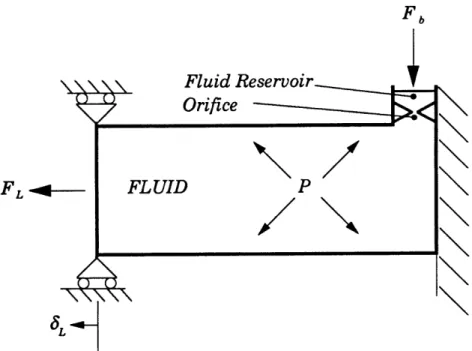
Figure 1.1 depicts the geometry of a pressurized vessel. The internal

pressure causes an elastic deformation, L,, or actuation force, FL, which

depend on the properties and dimensions of the vessel. An input force, Fb, controls the pressure via a piston-like mechanism. The fluid subjected to Fb is connected to the fluid in the vessel through a restricted passageway or orifice.

The actuation displacement, SL, is a linear function of Fb. If

constrained, an actuation force, FL, is a linear function of Fb multiplied by a ratio of the areas and dependent on the vessel properties. This

amplification effect is analogous to a hydraulic jack or a mechanical lever where a large pressure force is gained at the expense of a large input displacement. As the viscous fluid squeezes through the orifice, the fluid undergoes a shearing action and releases energy. This loss of energy is the source of damping.

(17)

Fb

Fluid Reservoir Orifice

F, FLUID P

SL

FIGURE 1.1: P-Strut Concept: An Elastic, Axially Deformable Body Under Internal Fluid Pressure

STATIC or ACTIVE

PASSIVE

FIGURE 1.2: Static, Active, and Passive Modes Of Operation

(18)

By tailoring the material properties of the vessel, the deformation or

the actuation force can be optimized. Furthermore, the type of actuation-elongation, bending, or torsion-are functions of the geometry and material properties of the actuator.

1.3 STATIC, PASSIVE, AND ACTIVE MODES OF OPERATIONS

The pressure actuator operates in three distinct modes which are illustrated in Figure 1.2. During static operation, where the velocity of the viscous fluid is negligible, the elongation, 8L, is linear with the input force,

Fb. Thus, the actuator could command and hold precise structural inputs

by maintaining a constant fluid pressure.

In the presence of dynamic structural disturbances, Fd, the actuator would be expanded or compressed generating SL independent of Fb. In order to accommodate the volume changes resulting from the disturbance,

the fluid in the vessel would be pumped or sucked through the orifice. The fluid shearing in the orifice would cause a damping of the disturbance. This mode of operation is passive.

The third mode of operation is active. If the input force, Fb, is

dynamic, the fluid in the reservoir would be forced into the orifice at a rate directly dependent on Fb. However, the viscous fluid is inhibited by the restricted passageway. Therefore, Fb applied slowly would allow the fluid to pass through the orifice and into the vessel (i.e. near static conditions); but with a rapidly applied Fb the fluid would not squeeze through. Thus, the actuator cannot command displacement or force at high rates or

(19)

the higher dynamics of a structure or amplifying back into a structure control system noise.

The technology needed to create and implement the pressurized fluid elastic actuator is available from "off-the-shelf" hardware. The concept is straightforward and an inexpensive, simple alternative to other actuator approaches.

1.4 APPROACH

The proposed pressurized fluid elastic actuator (dubbed the P-Strut) was designed with the objective of achieving actuation comparable to other available actuators. The dimensions of the P-Strut were optimized by solving the pressure-displacement relationships for pressure vessels. The investigation examined the advantages of tailoring the material properties to maximize the axial elongation. Analytical models were developed to represent the three modes of operation.

Three P-Struts were manufactured to prove the concept and demonstrate the benefits of customizing the material properties. The actuators were tested in each of the three modes operation for a variety of fluids and orifice diameters. The results correlated well with the models.

1.5 THESIS OUTLINE

This thesis describes the development and verification of a fluid elastic actuator.

(20)

Chapter 2 provides the background to controlled structures and discusses pneumatic piston devices which have been previously applied to the control of flexible structures.

The analytical groundwork for the design is presented in Chapter 3. The investigation begins by developing the pressure-displacement

relationships. The static performance equations, defined as input force, Fb, and input stroke, Sb, versus actuator displacement, 8L,, are derived in terms

of the P-Strut's material properties and physical dimensions. The viscous fluid and the orifice interaction is considered from solutions to channel flow problems. The three modes of operation are described via models which mimic the physics of the P-Strut. The parameters of these models include

elastic material and volumetric fluid stiffnesses, as well as a rate

dependent parameter (i.e. a dashpot) for the fluid-orifice effect. The models are used to define the appropriate mathematical equations. A parameteric study of the models emphasize the important parameters. The passive model was updated to account for an additional damping source discovered

during testing.

The equations developed in Chapter 3 are combined to determine the optimal actuator dimensions in Chapter 4. An isotropic, a composite-aluminum hybrid, and an all-composite P-Strut are described and optimally designed to demonstrate the advantages of tailoring the actuator's material properties. The "off-the-shelf" components of the P-Strut are discussed as well as the properties of the viscous fluids utilized.

Chapter 5 details the manufacturing procedures and the test methods. The construction included the chemical milling of aluminum tubes, and the layup of aluminum-composite (hybrid) and all-composite tubes. The method of filling the actuator with fluid is presented. The test

(21)

objectives and setup are described. The techniques and equipment utilized to determine the static, passive, and active performance of the P-Strut are discussed.

The experimental results are reported and correlated in Chapter 6. The performance of the three P-Struts with a variety of orifice and fluid combinations is presented. The static performance was linear. The active results compared favorably with the static results and the model developed in Chapter 3. The advantage of tailoring the material properties is

supported by the data. Passive damping, probably caused by the epoxy used in manufacturing, was discovered during testing. This damping

overshadowed the orifice damping.

A summary of the scientific and engineering benefits of this study conclude the thesis in Chapter 7.

(22)

CHAPTER 2:

Structures and Actuators in Structures

2.1 CHAPTER OUTLINE

This chapter presents a short review of flexible structures and the relevant aspects of structural control. A one degree-of-freedom

(1-DOF) model is used to explain issues involved in passive damping and active control. The use of an actuator in a feedback control system is

examined. Three general categories of feedback control are considered. Previous actuators which have used pressure as an actuation source are discussed and compared with the P-Strut concept. The differences between a piston pneumatic actuator and the fluid elastic actuator are clarified. Structural control issues surrounding the proposed fluid elastic actuator are presented.

2.2 THE CONTROLLED STRUCTURES FIED

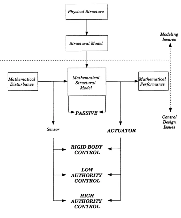
Figure 2.1 depicts an overview of the controlled structures field. Generally, a structure is first modeled with a set of assumptions and

(23)

Modeling Issures Structural Model

athematical Mathematical Mathematical Disturbance Structural Performance

Model PASSIVE Control Design Issues Sensor ACTUATOR RIGID BODY CONTROL LOW AUTHORITY CONTROL HIGH AUTHORITY CONTROL

(24)

estimated physical parameters. In reference 10, Craig published a broad survey of recent modeling topics and techniques. Modeling provides means to predict the performance of the structure and design a control approach.

2.2.1 A 1-DOF MODEL

A 1-DOF system consisting of a single mass, spring, and dashpot is

pictured in Figure 2.2. The model represents a structure with mass, M, elastic stiffness, K, and material damping, C, subjected to a disturbance

force, Fd. This system is useful for illustrating several significant

structural control concepts. The mathematical representation of the system is the equation of motion:

M + Cx + Kx = Fd (2.1)

or:

i+ 2Mi+ 2= Fd (2.2)

M

K C _

where: o. =- and = -w the structure's natural frequency

and damping coefficient, respectively. is a function of the material

damping parameter, C, which in turn is dependent on the material type,

and in some instances, on the loading [11,41,48]. For a typical structure,

4

is very small (0.1-1.0%).

An analysis of the model is usually accomplished in the frequency domain or the time domain [37,51]. In the time domain, assuming the

damping is negligible (4 =0), the equation of motion can be written as two

first order differential equations which together are called the state space equation:

(25)

S 0l 1

_-2_{_=}

x

t

₀

_+{}

F

-_d- _{= (X}=[AI{X)+[Bd]Fd} _(2.3)

X is the state vector (i.e. displacement and velocity), A is the system matrix, and Bd is the disturbance force mapping matrix which indicates how the force is directed into the states.

A frequency domain representation can be derived by taking the

Laplace Transform of 2.2 with zero initial conditions:

X(s) _ 02

( 2 + w 2 G(s) (2.4)

where G(s) relates the dynamic displacement X(s) to dynamic input Fd(s)

and the system parameters [37,51].

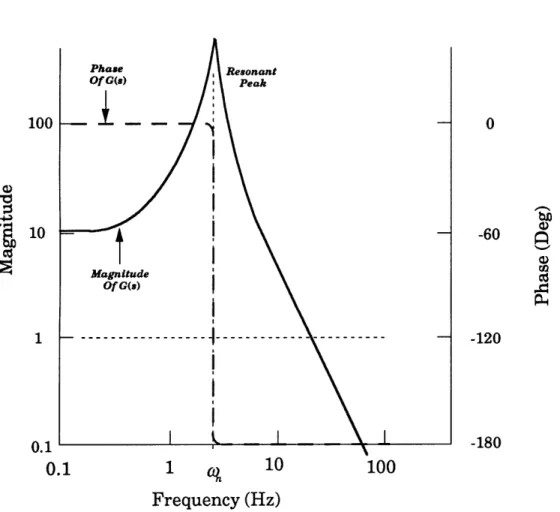
G(s) is the state transfer function [37,51]. The roots of the

denominator are called poles and the roots of the numerator are called zeroes. Two repeated poles are at w. The physical interpretation of a pole and zero can be observed from Figure 2.3, the Bode Diagram of G(s) [37,51].

The Bode magnitude and phase (i.e. the magnitude and phase angle of the sinusoidal response, X, to a sinusoidal input force, Fd) are depicted versus the complex frequency s. The peak in the magnitude and the shift in the phase occurs at o)n. This frequency location is labeled the natural

frequency, resonant frequency, or frequency of the structural mode. This frequency corresponds to a particular motion or mode shape of the

structure. For the system in Figure 2.2 the mode shape is the mass moving left to right. At an undamped pole the response to a disturbance would be infinite. If material damping is included ( 0O), the height of the peak and the sharpness of the phase shift are dependent on the inverse of [12,37,51].

(26)

x

1

C C

Material Damping Mass

FIGURE 2.2: 1-DOF Model

1 q 10 100

Frequency (Hz)

FIGURE 2.3: Bode Diagram of 1-DOF Model

100 0.1 0.1 0 -60 -120 -180

(27)

At frequencies approaching infinity the response rolls off to zero at an

average slope on a log-log scale of approximately the number of poles minus the number of zeroes [12].

2.2.2 A CONTROL APPROACH

The purpose of a control system is usually to minimize the

performance deviations and therefore minimize the associated deviations in the structural states. This amounts to controlling the modes of the system or reducing the resonant peaks of the transfer function. Usually, the approach to control design is to damp or move the resonant peaks which are critical to the performance.

To accomplish this objective the plant or modeled system must be paired with a control approach. The scheme could be as simple as adding passive components or designing a feedback control system using actuators and sensors. The type and level of control depends on the needed

performance.

Figure 2.4 depicts a typical feedback control diagram. The states are labeled X and are observed as the output of G(s) caused by the input of the combined disturbance force, Fd, and an actuator, F,. Y are the sensor outputs which are related to the states of the structure by a gain matrix Cy and are corrupted by a sensor noise N. The performance of the system, Z, is given by CX and consists of those states which should be controlled. The compensator loop gain and the dynamics of the actuator and sensors are combined in the compensator/actuator block, K,(s). The error, e, equals the difference between Y and the reference, r. If the gain and state

matrices are linear and constant, the system is linear and time invariant (abbreviated LTI) [37,51].

(28)

Performance

Gains Performance

Disturbance S s Actuator Force StatSensor

Force d States Noise

Error

F F X

r

_

K, (s)

-G(s)

C

-

y

Sensor Measurements

Compensator/Actuator Model Dynamics Dynamics

Feedback Loop

FIGURE 2.4: A Control System Diagram

To reduce the performance deviations as observed by Z, several types of control strategies are available, and research continues into new control strategies. However, for purposes of this discussion four generally well known approaches are examined: passive damping, rigid body control, low

authority control, and high authority control.

2.2.3 PASSIVE DAMPING APPROACH

Passive damping reduces the peak of the performance transfer function by increasing the system damping, C. In most instances, passive damping is added before feedback control and is thus independent of the control system. Passive damping changes the system transfer function G(s).

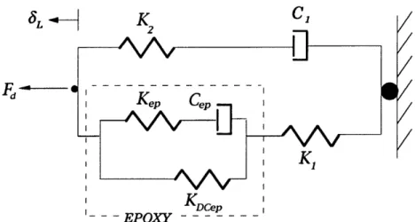
Figure 2.5 depicts a new structural model where a generic passive damping device has replaced the structural stiffness or spring element K in Figure 2.2. The damper is modeled as a pair of springs and a dashpot.

(29)

This model of a damper is representative of the passive mode of operation for the P-Strut. The device is in the load path of the structure and therefore must support the mass.

K1

M -F

C K

1 2

Passive Damper

Figure 2.5: Passively Damped System Model

The purpose of the damper is to add damping to the structure over a particular bandwidth. The dashpot and springs have a characteristic damping curve which offers significant damping within a limited

bandwidth. Inserting the device into the structure increases the damping coefficient of the system within the bandwidth of the device. In order to achieve the optimal reduction in the resonant peak, the frequency of

maximum damping within the bandwidth should be designed to match the resonant frequency. However, if the resonant frequency moves from the peak damping frequency, the damper is mistuned. The result is less, possibly insufficient, damping.

Damping is achieved by dissipating the energy in a system. Energy can be removed from the system through a strain mechanism. For

example a constrained viscoelastic layer attached to a structural member dissipates energy by shear strain. This mechanism offers reasonable damping with little mass penalty [3,39,49]. The Honeywell D-Strut-a

(30)

dashpot damper currently in operation aboard the Hubble Space Telescope--provides significant damping over a reasonable band of frequencies by displacing a fluid through a restricted passageway [2,9,14,35]. This damping concept is analogous to the P-Strut. A Piezo-resistive-shunted device, which when strained generates a voltage that is dissipated in a resistor, also offers damping over a moderate frequency range [20]. These types of passive devices have a fixed frequency at which the damping is maximum and a relatively broad band about this peak in which the damping is effective. In contrast, resonant dampers such as proof mass dampers or piezo-inductive-resistive-shunted devices are capable extracting a significant amount of energy and can be tuned to a particular frequency. However, these devices add additional modes to the system, and are only effective in a narrow band about the tuned frequency [20,29].

Although passive components are benign (i.e. they cannot add

energy), they are only capable of reacting to locally perceived displacements or forces and are independent of and unaware of the global performance.

2.2.4 ACTIVE CONTROL APPROACH

An adaptive structure requires control systems which can sense and command a structural change and compensate for unwanted changes. Figure 2.6 depicts the 1-DOF Model with an actuator in parallel with the structural stiffness. The active controller or compensator, KAs(s), in Figure 2.4 which controls the feedback gains and thereby the actuator response, Fa,

(31)

2.2.4.1 Rigid Body Control

Rigid body control involves deploying, retracting, or positioning an object. In order to accomplish a rigid body movement, an input

displacement is needed. If the mass is independent from the wall in the 1-DOF model (i.e. K=O in Figure 2.6), a commanded actuator displacement would cause the mass to move to a new position and hold. If the mass were truly rigid and no disturbance force was present the movement would be precise. However, if K O, or the mass has additional flexibilites not shown in the figure, the movement would involve a decaying vibration or ring

down around the displaced position. Preferably, an actuator would not add energy to the flexibility of the system. This can be accomplished either by input shaping, which diminishes the energy transmitted to the flexible modes of the structure by negatively reinforcing the resonant frequencies [45], or by an actuator which rolls off at frequencies lower than those of the flexibility of the mass. In a feedback control system, the measured states can be used to adjust the inputs and reposition or realign the structure via the actuator especially in the presence of disturbance force, Fd.

Ideal actuators are linear such that a feedback measurement yields a linear correction through the compensator. However, piezoceramics

exhibit mild hystersis effects and electrostrictives are quadratic (or higher) with respect to the driving voltage [4,13,32,50].

(32)

Structual Stiffness

K

x

M -F

C d

Actuator

FIGURE 2.6: System Model Actuator

2.2.4.2 Low Authority Control

Low authority control (LAC) decreases the resonant peaks in Figure 2.2 by actively adding damping to the structure. The objective is similar to that of passive damping; however, the achievable peak damping is higher and the frequency can be tuned. A proportional derivative (PD)

compensator feeds back a measurement of the displacement and the

velocity to influence both the natural frequency and system damping [37,51]. By properly designing the compensator, the structure can be significantly damped. A linear quadratic regulator (LQR), which is a full state feedback controller, accomplishes the peak damping for a single mode system in the same manner as the PD controller [12]. LQR is one type of modern control design technique. An advantage of modern controllers is the use of the state space representation (equation 2.3) which is optimal for computer implementation. The deviations in performance can be written as a cost which can be minimized by mathematical operations resulting in a stable compensator design. [12,37,51].

Regardless of the compensator, the actuator must be capable of commanding an input at the frequency of the mode which is to be damped. The frequency bandwidth over which the component can actuate dictates to

(33)

what frequency and to what extent active damping is possible. If the actuator cannot command force or displacement at a particular frequency no damping or control is possible. Therefore, care must be exercised in selecting the appropriate actuator. Piezoceramic materials and

electrostrictives are capable of excitation over a broad range of frequencies [46]. At frequencies out to 1K Hz, Scribner, et.al. employed a piezoelectric component to isolate transmitted disturbances in a model of a rotor blade [44]. At lower frequencies (< 25 Hz), Hallauer, et.al. used an air jet thruster alone and paired with a reaction mass actuator to damp a planar truss

[22,23].

2.2.4.3 HIGH AUTHORITY CONTROL

High authority control (HAC) involves shifting the structural frequencies and altering the mode shapes of the structure [12]. HAC means moving the peak and lowering the entire curve in Figure 2.3

therefore, greatly diminishing the performance deviations. The magnitude of the commanded input must be comparable to the disturbance. In

essence, HAC attempts to cancel the disturbance such that from Figure 2.6, Fa=-Fd. HAC can involve a multi-input-multi-output problem with many

actuators and sensors. HAC compensators can be determined from frequency weighted cost functions including techniques to handle parametric uncertainties and unmodeled dynamics [12].

(34)

2.3 PREVIOUS APPLICATIONS OF PRESSURE ACTUATORS IN STRUCTURES

Due to the inherent bandwidth limitations on pneumatic or pressure-type actuators, structural applications have been limited. Sievers and VonFlotow appropriately dismissed pneumatic actuators in developing an isolator for damping acoustic vibrations [46]. Nevertheless, pneumatic actuators have been successfully used at low frequencies.

Rafati designed and tested a pneumatic piston actuator with

application to passenger trains [40]. His component was utilized in a LAC system to damp modeled disturbances transmitted from the rail to the train. These disturbances included the accelerations due to train rocking and bouncing and occurred at frequencies below 5 Hz. The opening and closing delays in a solenoid valve limited the performance of his system. The pneumatic air-jet developed by Hallauer and Smith-used to damp a planar truss-expelled pressurized air to generate a force (i.e. thrust). The air-jet had a limited bandwidth due to delays in opening and closing the air valve [22].

Lim, et.al. used unspecified pneumatic actuators in comparing three multi-input-multi-output control systems. The structure consisted of a fifty-one foot truss connected to a sixteen foot diameter reflector with the highest controlled frequency of 1.87 Hz [30]. His results suggested that a PD type controller with feedback to the pneumatic actuators compared favorably to other controllers.

Karnopp proposed an active and passive-active isolation system for a high-speed ground vehicle using a modern control theory approach [26].

(35)

Butsuen proposed a semi-active isolation system to isolate roadway disturbances without severely limiting an automobile's handling characteristics [7]. Since a substantial force is required over a modest bandwidth, these control systems could involve a fluid elastic actuator.

2.4 THE P-STRUT VS. PREVIOUS PRESSURE ACTUATORS

The proposed P-Strut commands a force or displacement by

controlling the internal pressure in an elastic deformable cylinder. On the other hand, the piston actuator developed by Rafati used a solenoid to open and close a pressurized chamber. Hallauer's air-jet released a directed stream of high pressure air to generate on/off thrust.

The proposed fluid elastic actuator has an inherent frequency roll-off similar to other pneumatic actuators. However, in the P-Strut the

bandwidth is limited by the fluid-orifice interaction, whereas in piston actuators and the air-jet, the frequency bandwidth is limited by the opening and closing of the solenoid valves [40,22]. Moreover, the viscous fluid adds passive damping qualities. When not actuating, the P-Strut is capable of absorbing energy, thus further improving the performance of the structure. In contrast, the air-jet and piston actuators are not designed to add passive damping.

(36)

SP1TZi

GROY)7cD2

CHAPTER 3:

Developing the Performance Equations

3.1 CHAPTER OUTLINE

This chapter examines the physical principles of the P-Strut and develops the mathematical equations which describe the actuator's three modes of operation: static, passive, and active.

Section 3.2 describes the dimensions of the P-Strut that are relevant to the analyses.

In Section 3.3, the pressure-strain relationships are developed via the stress-strain constitutive equations for isotropic and anisotropic materials. The axial elongation of the structure is determined as a function of the input force and input stroke. These equations define the static performance of the actuator. Anisotropic material properties are shown to enhance the performance.

Section 3.4 investigates the damping interaction between the viscous fluid and the orifice. An effective loss coefficient is estimated by

(37)

considering laminar and turbulent channel flows. In addition, accelerating and sinusoidally varying pressure flows are examined.

A mechanical analysis details the passive mode of operation and leads to a three parameter model in Section 3.5. The parameters include

discrete elastic and volumetric stiffnesses, as well as a dashpot representation of the fluid-orifice interaction. The physical and

mathematical development indicates that these stiffnesses compete against one another reducing the passive damping. The P-Strut performance is compared to the Honeywell D-Strut and piezoelectric resistive-shunted struts. The passive model is updated to include the additional damping encountered during testing. The revised model based on the measured performance has damping which overwhelms the predicted orifice damping.

Section 3.6 examines the active performance of the P-Strut. A second discrete stiffness model is developed with similar physical parameters. Mathematically and physically, the model defines the non-collocated transfer function between the input force and the actuation displacement. The static performance, as well as the frequency roll-off due to the fluid and orifice, are properly incorporated into the model. A parameteric study demonstrates the important parameters.

(38)

3.2. DEFINITION OF THE P-STRUT GEOMETRY

Figure 3.1 depicts a schematic of the P-Strut. The fluid-elastic

actuator is a circular cylindrical pressure vessel which is sealed with rigid flat-plate endcaps. The fluid inside the cylinder is connected via an orifice to the fluid inside the reservoir or flexible bellows.

The cylindrical actuator has a length L, with inner radius Ri, outer

radius Ro, and thickness t. R, represents the average radius or (1/2)(Ri +Ro).

Since t<<R,, the three radii are approximately equal (i.e. Ro=R'=R,). Thus, the cross-sectional area, Ac, and the annulus or vessel wall area, Aa, can be expressed as:

A = zR2 = 7R2

(3.1)

A. = 7(R - Rj ) = 2 7Rt

The bellows is depicted in Figure 3.2. The reservoir or bellows has an

effective cross-sectional area Ab. This dimension is difficult to compute

from the geometry of the bellows. (In this study, Ab is determined directly

from the experimental results.)

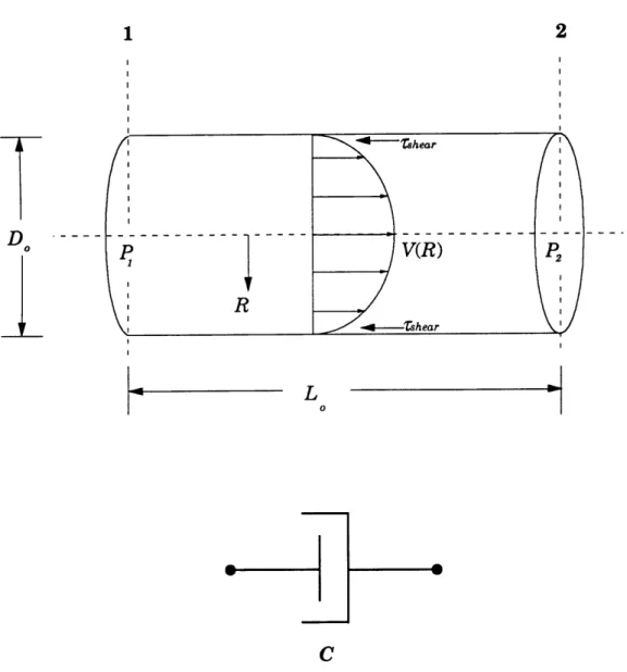
The orifice has cross-sectional area Ao and length Lo.

The ratio of the P-Strut cross-sectional area, Ac, to the effective

bellows area, Ab, equals the fluid lever introduced in Chapter 1. This fluid

lever is represented by Yb. The ratio of A, to the area of the orifice, A0, is

defined as Wo. Ab divided by Ao equals Yob. As equations:

A=

A b Ab

(39)

ORIFICE P-STRUT CIRCULAR CYLINDER

tENDCAP

ENDCAP A = Annulus Area A = Interior Area CIRCULAR CYLINDER

FIGURE 3.1: Description of the P-Strut Geometry

39 ENDCAP FLUID 1LLJ~ I U U RC

(40)

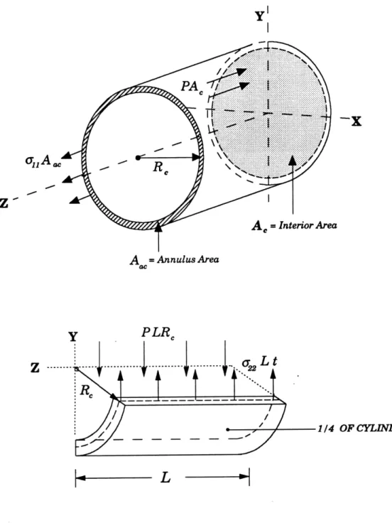
Figure 3.3 depicts the element ABCD extracted from the surface of the P-Strut cylinder illustrated in Figure 3.1. The longitudinal direction is labeled L or 1 and the hoop direction is labeled H or 2. The curvature of the element in the hoop direction is R. The element is not curved with respect to the longitudinal direction.

3.3 DERIVATION OF THE STATIC EQUATIONS

As established in Chapter 1, the P-Strut is an elastically deformable pressure vessel. The static analysis derives the elongation of the P-Strut

(i.e. actuation authority) as functions of the input force and stroke.

3.3.1 CONSTITUTIVE EQUATIONS

In general, the application of an arbitrary load induces normal and shear stresses in the cylinder wall which can be described in the 1, 2, and 3 coordinate directions. However, since the thickness of the cylinder, t, is much smaller than the radius, Re, the stresses through the thickness are negligible (i.e. a,,2, a,,3, and u33=O). With this plane-stress state assumption,

the constitutive equations are:

[]

E1111

1122

2E1112

E

22 = E1122 E2222 2E2212 22 (3.3)

a12 E1112 E2212 2E1212 12

or abbreviated:

(41)

BELLOWS

ORIFICE

, , Effective Bellows Area

SA

b

Lb

Ao ₀= Area Orifice

FIGURE 3.2: P-Strut Bellows and Orifice Geometry

ELEMENT

ABCD

H or 2

CENTER OF CYLINDER

FIGURE 3.3: Definition of Longitudinal (1) and Hoop (2) Coordinate Directions

(42)

The components of the E matrix represent the cylinder's material

properties. The 2 appears in the last column of E since the tensor strain,

e12, instead of the engineering strain, 12, is used.

If a pair of orthogonal planes of material property symmetry exists, the material is categorized as orthotropic. Defining the material properties in these orthogonal or principle directions, E1 112=E2212=O. This eliminates

the coupling between the normal stresses and the shear strain. Rewriting matrix equation 3.3 with orthotropic material constants, yields:

471 E1111 E1122 0 Ell

11 Ii (3.5)

-22- E2222 0 .225)

a12 sym 2E 1 2 1 2 £ 12

Equation 3.5 can be expressed in terms of the vessel wall's engineering properties as:

I

11

Ell V21El

0 E

2 2 1 E22 0 e22 (3.6)

12 - 1 Dsym 2G1 2 (- 12 2 1 12

where Egl and E22 are the Young's Modulii and v12 and v21 are the Poisson's

Ratios in the 1 and 2 coordinate directions. These four engineering constants are related by the expression v12E22=v21E11.

Inverting and expanding matrix equation 3.6 to solve for the strains: [ll

C

₁₁₁1 C₁₁₂₂ 0

a

l

22 2222 0

H

22 (3.7)

12 sym 2C1212 U1 2

(43)

1 1

C1111 C2222 =

1122 _Ell _E22 ₁₂₁₂

4G12

For an isotropic material, El'=E2=E, v12=v2 1=v, and G12=E/[2(1+v)].

Thus, only two constants are required to characterize the constitutive relationships for a material such as aluminum. Combining 3.8 and 3.7, the isotropic longitudinal strain can be written as:

S= 1(a - v 22 ) (3.9)

E and the hoop strain as:

e22 = E( _{2 2}- vo1 1) (3.10)

E

An actuator constructed from composites would, in general, have anisotropic material characteristics. Composite laminates are

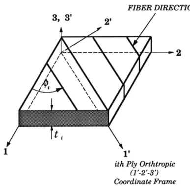
manufactured from individual plies which posses material properties aligned in their fiber and transverse fiber directions. In order to determine the material properties in the laminate reference frame (1-2), the

contribution from each ply must be considered.

From Figure 3.4, a ply coordinate system (1'-2') is defined at an angle, P, from the laminate coordinate frame. In the 1'-2' directions, the

ply orthotropic material constants, E'ail, are defined as:

E E' El E' 22 E1111 = 1- v2 ,21 ₂₂₂₂ 1- 2 1 ( (3.11) v2E_ E2 =G - v21 ₁₂₁₂ 1122 1212 _1v2212_V21

(44)

FIBER DIRECTION

--- --- 2

1 1'

ith Ply Orthtropic (1'-2'-3') Coordinate Frame

FIGURE 3.4: Typical Composite Laminate Layup

To transform the ith ply's E' t into the 1-2 laminate frame, four invariant constants are needed [17,25].

I, = (1/ 4)[E + E222' +2E1122

2 = (1/ 8)[E _{2 2 2} - 2E ₁₂₂+4E1₂₁₂

E2222 1122 _(3.12)

I, = (1/ 2)[E;111 - E2222]

I4 = (1/ 4)[El11 + E2222 -2E122 - 4E1212]

With these invariants, the ith ply's material constants are transformed into the 1-2 coordinate system:

E1111i =I, + I2 + I3 cos(2 (P) + I1 cos(4 '~) E2 i= I + 12 - 13 cos(2 (P) + 14 cos(4 (P)

E1122 = I1 - I2 3- cos(4 () (3.13)

E,212 = 2 - I cos(4 (P1)

E12= (13 / 2) sin(2 V'i) + I4 sin(4 9')

(45)

With the rotated Eg, in the laminate coordinate frame, a thickness weighted stiffness matrix, A, can be determined by adding individually the stiffnesses of equation 3.13 multiplied by the ith ply's thickness:

The average

t- # ples

Aap, = Ear'dt EaCd(Ep=r')t#=

ti-1 i 1

laminate stresses, oL, are defined as:

C C12 L A A 2A1112 11

lT4

=

A

₂₂₂₂

2A

2212 22 12 sym 2A_{1 2 12} 12 or, abbreviated: 1 (oL ) = - [AI(E) t (3.14) (3.15) (3.16)

For a balanced laminate, where the number of -(P plies equals the

number of +9P plies, A1112=A2212=O (i.e. the material is quasi-orthotropic).

Inverting 3.16 for the strain vector:

{e) = t [A]- 1_{(' )} _(3.17)

Assuming a balanced laminate, equation 3.17 can be expanded as: e11 e22 e12 0

U1{

L

O of2 (A1111A2222 - A1122)/4 "12 sym (3.18) where A = A_{12 12}(A 1 1 1A2 2 2 2 - A122)

Equation 3.18 is analogous to equation 3.7. Defining the effective laminate compliance matrix CL as:

[CL ] = t [A]-1 (3.19)

-A1122A1212

(46)

the effective or "smeared" laminate engineering properties can be determined from equation 3.8 as:

EL=

1

1 = - 111122 1 E2 L 2222 2L = -E 1122 V21 C"2 1 4Cf_{1 2}

where the elements of CL are defined in equation 3.7.

With 3.17 and 3.20, the longitudinal and hoop strains are defined as:

E = ( l - V22) 11 E₂₂ =2 - v( c 1) EZZ22 1 3.3.2 As acting in

PRESSURE -STRAIN RELATIONSHIPS

illustrated in Figure 3.5, the longitudinal and hoop stresses the walls of a thin pressurized cylinder are:

L _ PR 2t 2 L _PR U22 (3.21) (3.22) (3.23) (3.24)

These equations are derived by equilibrating the forces acting in the 1 and 2 directions (i.e. the pressure force versus the stresses in the cylinder wall).

Substituting 3.23 and 3.24 into the isotropic strain equations 3.9 and

3.10 yields the longitudinal strain as a function of the internal pressure: PR

ell =- (1-2v) (3.25)

2tE

(47)

a6

1

A

A _OC= Annulus Area PLRC Z ---S...iiiiiii AC = Interior Area ;2Lt ,/ 1/4 OF CYLINDER

L

-FIGURE 3.5: Pressurized Circular Cylinder

(48)

and the hoop strain:

= PR (2- v) (3.26)

2tE

Similarly, substituting 3.23 and 3.24 into the quasi-orthotropic strain equations 3.21 and 3.22 results in the composite longitudinal and hoop strains: PRu = (1- 2 v2 ) _(3.27) Ell 2tE11 e22 2tE(2- v2L) (3.28) 2tE2

The ratio of longitudinal to hoop strain is defined as F. The isotropic

strain ratio, FI, equals 3.25 divided by 3.26, or:

i = 11 (1-2v) (3.29)

e22 (2- v)

The ratio of the composite strains, equation 3.27 versus 3.28, is defined as:

S= __ - E_{2 2}L( -2 12L) (3.30)

e22 EL (2 - 21L )

3.3.3 DERIVATION OF THE ACTUATION AUTHORITY, INPUT FORCE,

AND STROKE REQUIREMENTS

From the elementary definition of strain, the actuation displacement

of the P-Strut, 8L,, is given by:

3L = LLff eli (3.31)

where Lef is the effective length of the actuator. The effective length is the length over which the longitudinal strain acts plus a contribution due to the end conditions. Near the boundaries the pressure-stress equations 3.23 and

(49)

3.24 are not valid. In order to satisfy compatibility at the boundaries, additional moment and shear stress-resultants, acting out of the 1-2

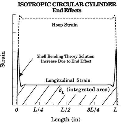
coordinate plane, must exist. These resultants can be solved using linear Shell Bending Theory which predicts a dramatic increase in e,, near the end conditions [16,27]. In essence, the clamped-rigid endcaps physically restrict the radial swelling or the hoop strain of the vessel (see Figure 3.6). As the hoop strain is diminished near the boundary, the local longitudinal strain is increased due to Poisson's effect.

Figure 3.7 depicts the strains as a function of the position calculated using a complete Shell Bending Theory solution. The peaks in E,, near the ends of the cylinder correspond to the end effects and the reduction in hoop strain while the dominating plateau in e,, is the strain predicted by the elementary pressure-strain equations 3.25 or 3.27. Therefore, over the majority of the cylinder the simplified pressure-strain equations 3.25 and 3.26 or 3.27 and 3.28 are valid; only near the ends does the solution require the more complicated bending theory approach. The Shell Bending Theory solution is reported in Appendix A and analyzed extensively (for isotropic and anisotropic cylinders) by Graves in reference 18.

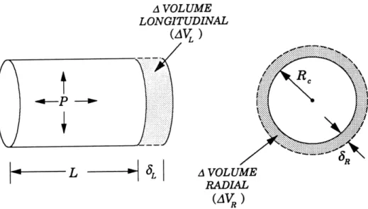
The elongation, 8L, equals the longitudinal strain integrated over the

length of the P-Strut. The peaks in e, at the boundaries are accounted for by adding an amount t to the physical length of the P-Strut, L, i.e.:

Design of a fluid elastic actuator with application to structural control

DESIGN OF A FLUID ELASTIC

ACTUATOR WITH APPLICATION TO

STRUCTURAL CONTROL

Aero

'JUN

08 1993

DESIGN OF A FLUID ELASTIC

ACTUATOR WITH APPLICATION TO

STRUCTURAL CONTROL

Acknowledgement

Table of Contents

List of Figures

List of Tables

Nomenclature

Ao

E,

K

K,

Ks

KDCp

Lo

6

a,

r

CHAPTER 1:

A Fluid Elastic Actuator

SL

CHAPTER 2:

Structures and Actuators in Structures

4

S 0l 1

x

t

+{}

F

x

1

r

_

K, (s)

-G(s)

C

-

-

y

K

x

SP1TZi

GROY)7cD2

CHAPTER 3:

Developing the Performance Equations

A=

tENDCAP

[]

E1111

2E1112

I

Ell V21El

0

E

C

a

l

H

lT4

=

A

2A

U1{

L

1

a6

A

L

_+{}