Verification of the Coupled-Momentum Method with Womersley's Deformable Wall Analytical Solution

HAL Id: hal-02414672

https://hal.inria.fr/hal-02414672

Submitted on 16 Dec 2019

HAL is a multi-disciplinary open access archive for the deposit and dissemination of sci-entific research documents, whether they are pub-lished or not. The documents may come from teaching and research institutions in France or abroad, or from public or private research centers.

L’archive ouverte pluridisciplinaire HAL, est destinée au dépôt et à la diffusion de documents scientifiques de niveau recherche, publiés ou non, émanant des établissements d’enseignement et de recherche français ou étrangers, des laboratoires publics ou privés.

Verification of the Coupled-Momentum Method with

Womersley’s Deformable Wall Analytical Solution

Vasilina Filonova, Christopher Arthurs, Irene Vignon-Clementel, C. Alberto

Figueroa

To cite this version:

Vasilina Filonova, Christopher Arthurs, Irene Vignon-Clementel, C. Alberto Figueroa. Verification of the Coupled-Momentum Method with Womersley’s Deformable Wall Analytical Solution. Inter-national Journal for Numerical Methods in Biomedical Engineering, John Wiley and Sons, 2019, �10.1002/cnm.3266�. �hal-02414672�

Verification of the Coupled-Momentum Method with Womersley’s

Deformable Wall Analytical Solution

Vasilina Filonovaa*, Christopher J. Arthursc, Irene E. Vignon-Clementel d,e, C. Alberto Figueroaa,b,c a

Surgery and b Biomedical Engineering,University of Michigan, Ann Arbor, MI, USA

c _{Imaging Sciences and Biomedical Engineering, King’s College London, UK} d

Inria, Paris, France

e

Sorbonne Université UPMC, Laboratoire Jacques-Louis Lions, Paris, France

Abstract

In this paper, we perform a verification study of the Coupled-Momentum Method (CMM), a 3D fluid-structure interaction (FSI) model which uses a thin linear elastic membrane and linear kinematics to describe the mechanical behavior of the vessel wall. The verification of this model is done using Womersley’s deformable wall analytical solution for pulsatile flow in a semi-infinite cylindrical vessel. This solution is, under certain premises, the analytical solution of the CMM and can thus be used for model verification. For the numerical solution, we employ an impedance boundary condition to define a reflection-free outflow boundary condition and thus mimic the physics of the analytical solution, which is defined on a semi-infinite domain. We first provide a rigorous derivation of Womersley’s deformable wall theory via scale analysis. We then illustrate different characteristics of the analytical solution such as space-time wave periodicity and attenuation. Finally, we present the verification tests comparing the CMM with Womersley’s theory.

Keywords: Verification; Womersley Deformable Wall Solution; Coupled-Momentum Method; Impedance Boundary

Condition; Blood Flow; Fluid-Structure Interaction.

1

Introduction

Blood can be represented as an incompressible fluid whose constitutive behavior is usually approximated, at least in the larger arteries, by a Newtonian model and the incompressible Navier-Stokes equations. Blood velocity, pressure, and propagation of waves within the arterial tree are greatly affected by the deformability of the vessel wall 1,2. Wave speed and changes in amplitude and phase are dictated by vessel size, viscoelastic behavior, and by blood viscosity. Wave attenuation and dispersion are also observed within the cardiovascular system.

Numerous mathematical formulations have been developed to represent these complex physical phenomena, usually describing oscillatory flow in an idealized tube, rigid or elastic 3–8. One of such formulations is given by Womersley’s analytical velocity profile for oscillatory flow in rigid tubes 9. This was then extended to the case of compliant arteries by taking into consideration wall deformations and radial components of blood velocity, producing an analytical solution for pulsatile flow in a deformable, axisymmetric, semi-infinite vessel 9–13. Womersley’s deformable wall analytical solution represents an excellent framework to understand some of the governing principles of wave propagation phenomena in the cardiovascular system. It is also a good tool for performing verification studies of mathematical models of blood flow in compliant arteries.

Beyond analytical solutions, computational 3D models have been used extensively to study fluid-structure interactions (FSI) between blood flow and vessel wall motion. Boundary-fitted techniques

*

Corresponding author at: University of Michigan, North Campus Research Complex, 2800 Plymouth Road, build. 20 – 203W-1A, Ann Arbor, MI 48109.

based on Arbitrary Lagrangian-Eulerian (ALE) formulations 14–16, non-boundary fitted techniques such as the Immersed Boundary Method 17,18 or the Fictitious Domain Method 19, or simplified models such as the Coupled-Momentum Method (CMM) 20,21 have been proposed to describe cardiovascular FSI. These are all complex formulations which require rigorous benchmarking to ensure error-free implementations.

There are several studies that have used analytical solutions for pulsatile flow in compliant vessels for validation and verification of 3D computational FSI models 22–26. A FSI strategy involving external coupling of ANSYS and CFX solvers for blood flow in a straight elastic tube was compared against a single-frequency Womersley’s analytical solution 22. Verification and validation of a FSI numerical method based on OpenFOAM was described in the work of Kanyanta et al. 23, comparing numerical results with analytical expressions for pressure wave speed and axial stress perturbations 27,28, as well as with data from polyurethane mock artery experiments. In the paper of Passerini et al. 26, validation of the open-source LifeV framework was presented with verification against an analytical solution for wave speed. Ponzini and colleagues 24 presented an in vivo validation using 2D Phase Contrast Magnetic Resonance Imaging of a Womersley number-based formula for estimating flow rate in several arteries. In the study of van Geel et al. 25, an ALE FSI numerical model with viscoelastic walls was compared against Womersley’s solution and experimental results, showing good agreement for straight and tapered vessels.

The purpose of this paper is to perform a verification study of the CMM 20 against a multi-frequency Womersley deformable wall analytical solution. The CMM is 3D method that considers a monolithic approach for the FSI problem, a thin linear elastic membrane model for the arterial wall, and fixed conforming meshes at the vessel wall-fluid boundary interface. The dynamic coupling between blood and vessel wall was achieved by defining a fictitious body force driving the wall motion, similar to a key assumption in Womersley's deformable wall analytical solution 13.Womersley's deformable solution can be regarded as the analytical solution for the Coupled-Momentum Method under the following conditions: cylindrical and axisymmetric geometry; linear, periodic flow, and non-reflective outflow boundary conditions. Therefore, it is best suitable for verification.

A key component of this work is the utilization of an impedance boundary condition for the outflow boundary of the computational domain 29. This approach makes it possible to use a reflection-free outflow boundary which can mimic the physics of the analytical solution, defined on a semi-infinite domain 30. Furthermore, this approach for outflow boundary condition avoids the direct specification of any of the main solution variables at this boundary, and thus contributes to a more rigorous set-up for the verification of the CMM.

The structure of this paper is as follows. In the methods section, an overview of Womersley’s analytical solution for pulsatile flow in a deformable, axisymmetric, semi-infinite cylindrical vessel is provided first in Section 2.1 13. This is complemented by Appendix where the mathematical formulation is recapitulated in concise, non-dimensional form applying scale analysis 31 to summarize the theory’s limitations needed for verification. The CMM 3D formulation is then presented in Section 2.2. Special care was taken to define a non-reflective boundary condition for the numerical domain, using a coupled-multidomain method 29. In the results section, first in Sections 3.1-3.2 a multi-frequency Womersley deformable solution is determined, in order to represent flow, pressure and wall motion in an idealized model of a human common carotid artery. Finally, in Section 3.3 numerical solutions of the CMM were compared against the analytical solution. Special care was taken in the definition of the problem parameters to ensure that solutions are both physiologically realistic and compatible with the assumptions of Womersley’s theory.

2

Methods

In this section we carefully describe the assumptions and governing equations leading to Womersley’s theory and to the CMM method. We focus on the main assumptions relevant for the comparison of the methods. For example, Womersley’s theory is described on a semi-infinite cylindrical vessel using 2D axisymmetric assumptions and linear fluid-solid interactions. Conversely, the CMM is a numerical formulation capable of dealing with 3D geometries and nonlinear flows on finite domains. However, under certain assumptions the CMM can be reduced to the Womersley’s deformable wall formulation. These assumptions include: axisymmetric linear flow, straight elastic vessels with thin walls, a total wall surface traction used to define a wall body force, and no wave-reflections. The latter assumption is enforced in the finite numerical domain via an outflow impedance boundary condition.

2.1 Womersley theory for blood flow in a deformable vessel

The Womersley’s theory describes the axisymmetric motion of blood when subjected to a periodic pressure gradient in a straight elastic vessel. Under a linear assumption, the pumping action of the heart results in a pressure gradient k_total, which can be decomposed into a constant component k_s producing a steady forward flow, and an oscillatory component

k

with zero net flow over the cardiac cycle 32:

( , , ) ( , , ) total total s p k r z t k k r z t z      , (1)

where p_total is a total pressure field with steady and oscillatory contributions; r and z are the radial and longitudinal coordinates of the tube, respectively, and t is a time variable.

The total velocity field in the longitudinal and radial directions can be written as: Longitudinal: ( ) ( , , )



2 2



( , , ) 4 s total s k w w r w r z t r R w r z t       , (2) Radial: u_total u r_s( )u r z t( , , )u r z t( , , ), (3) where w and u are the oscillatory components of the velocity field. The steady Poiseuille longitudinal component

s

w is added to w to reconstruct the total velocity profile. In the radial direction, the steady component of the velocity u r_s( ) is identically zero. Here, R is the vessel radius and



is the blood dynamic viscosity. Similarly, the total pressure field p_total can be decomposed in terms of its steady, p_s, and pulsatile,

p

, components as:

0

( ) ( , , ) ( , , )

total s s

p p z p r z t p k z p r z t , (4) where p₀ is the mean temporal pressure at the inlet of the vessel (z 0).

The complete derivation of Womersley's governing equations for a freely-moving elastic, cylindrical and semi-infinite vessel 13 is presented next. The presented derivation refers only to the oscillatory components of the velocity and pressure field (

w u

,

, and

p

). A scale analysis (order of magnitude analysis) 31 of the governing equations is used to understand the validity limits of the simplifying assumptions of theory. The following scaling rules were considered for blood flow and vessel wall variables:

2 , c , t , , , , r R r z z t u



cu w



cw p



c p





            (5) , , c c







 









   (6)

where  is the angular frequency of oscillations, c is the wave speed,  is the blood density, and   , , are non-dimensional scale parameters for the longitudinal velocity, radial velocity, and pressure, respectively.  and  represent the oscillatory radial and longitudinal displacements, respectively. In equations (5) and (6) all non-dimensional variables, denoted by primes, are assumed to be of the same order ~ (1).

2.1.1 Blood flow equations

In a cylindrical system of coordinates and using the non-dimensional form (5), the mass balance equation and Navier-Stokes equations for momentum balance in the radial and longitudinal directions are given by: 0 u u w r r z              , (7) 2 2 2 2 2 2 2 2 1 1 u u u p u u u u u w t r z r r r r r z                   _{ } _{ } _{ }  _  _  _{ }             _   _  _      _, (8) 2 2 2 2 2 2 1 1 w w w p w w w u w t



r z



z



r r r



z             _ _      _  _    _   _        _   _  _     _, (9)

where the non-dimensional parameter



R

 

is the Womersley number, and    is the blood kinematic viscosity.

The Navier-Stokes equations (8), (9) can be significantly simplified under the long-wave approximation assumptions, namely: 1) the characteristic flow wavelength  2 c  is much larger than the vessel radius R ; 2) the wave speed c is much larger than blood velocity components. From the first condition, it follows that the non-dimensional scale parameter  R/ c 1; and from the second condition the velocity scale parameters introduced in eq. (5) should be small:  , 1. Moreover, from (7) the following relations apply to scale parameters, oscillatory velocities, and coordinates:

1, u u 1, r r 1. w w z z



_

_

_



          (10)

All non-dimensional variables in eqs. (8), (9) are (1) due to the scaling rule. The non-linear term (advective inertial forces) are (



) and the viscous stress axial terms are (



2) and can thus be neglected. The simplified momentum balance equations become linear and therefore amenable for superposition of solutions in a harmonic wave form.

Boundary conditions for the fluid problem include: no-slip at the fluid-solid interface (e.g. matching velocities of fluid and solid at the wall), imposed oscillatory velocities ˆu and ˆw at the tube inlet, and finite velocity at the vessel centerline.

Remark 1. When performing the verification study of the CMM, it is important to estimate the

contribution of the non-linear advective term present in the numerical solution but absent from the analytical solution. The non-dimensional scale parameter



can be estimated from (5) as  w c, where ( , ) ( , , )

R

w z t  w r z t is the averaged longitudinal velocity over the radius. The oscillatory flow rate can be written as q z t( , ) R w z t2 ( , ). The upper bound of the non-linear advective scale parameter of the numerical solution num can be estimated from the maximum oscillatory flow at the inlet

q

inp as

[0, ] 2

max _totalinp _s

t T num num q q R c      , (11)

where q_totalinp q_s q z( 0, )t qinp, and cnum is the reconstructed wave speed from the numerical solution.

In addition, to check satisfaction of u c 1, one may estimate   , utilizing relation (10).

Remark 2. Radial and longitudinal pressure gradients should not be neglected to obtain non-trivial

velocity solutions. These terms, scaled by



and  2 in eqs. (8), (9), are preserved since they do not affect the linearity of the equations regardless of their order, but they do affect the solution.

2.1.2 Vessel wall equations

The vessel wall equations of motion are written in the context of linear elasticity and thin-walled tube theories, assuming small radial deformations. Cauchy’s equation of motion is w 2 2

t

       F T ,

where w

is the wall density, F a body force per unit volume, T the Cauchy stress tensor for the vessel

wall, and , 0,

T

 

 

  

 is the oscillatory displacement vector in cylindrical coordinates. The thin-wall assumption states:

, ,

h R  R (12)

where h is the vessel wall thickness. The solid domain is modeled as a membrane and thus a 2D interface with the lateral boundary of the fluid domain. Relations (12) imply small radial deformations and thus the average radial coordinate of the vessel wall is r R. Therefore, a no-slip kinematic boundary condition at the fluid-solid interface, r R, is simply

r R

u  t

    , wr R    t .

Further exploiting the thin-wall assumption, Womersley defined radial and longitudinal components of a fictitious body force F driving the dynamics of the membrane from the pressure p and shear stresses

 acting on the lateral fluid boundary as:

, r R r z r R p _{u w} F F h h h z r             _  _     . (13)

The stress tensor

T

is defined by considering two stress states: internal pressurization with no axial strain, and axial force with no internal pressure. The linear superposition of these states yields the following circumferential and longitudinal components of the stress tensor 13:

, _zz T B T B R z R z   _  _          _  _  _  _      , (14) where



2



1

B E  ,

E

is the Young's modulus of the vessel wall, and  is its Poisson's ratio. Using eqs. (5),(6),(12),(13) and neglecting smaller terms in the divergence of the stress tensor,



 T



r  

 

T r _{r R} and



 T



z  Tzz z, we obtain the radial and longitudinal equations of motion

for the vessel wall in non-dimensional form: 2 2 2 w r 1 w 2 , R B p z t h c                _{   }   _{ }   _{ } (15) 2 2 2 2 2 2 1 . w w r u w B z r z t h R c z   _{ }     _            _{ }  _  _  _     _{   } _{   }    _{  }  _ (16)

The non-dimensional coefficient 2

( w ) 1

B  c  because the velocity of shear waves in the material of the tube is greater than the pulse wave velocity 13. Using long-wave approximation, 2 1, equation (15) can be reduced to a radial equilibrium equation. Similarly, the term  u z in eq. (16) can be neglected.

Remark 3. The small deformation assumption in eq. (12) does not apply to the axial direction, in which

the longitudinal deformations can be finite. Womersley developed an extension of the theory 11 where an additional longitudinal wall motion elastic constraint was introduced to reduce axial wall deformations, see Remark 5.

2.1.3 Summary of fluid-solid equations and solutions

The resulting non-dimensional, linear system of second order differential equations for the fluid-solid problem is summarized in Erreur ! Source du renvoi introuvable.. The solution in harmonics waves is completely derived in Appendix A.1 and summarized in Erreur ! Source du renvoi introuvable.. The wave speed c is defined by frequency equations as described in Appendix A.2. Initial conditions for velocity, pressure, and wall displacements must be provided. Lastly, velocities at the center of the vessel are assumed to be finite, Erreur ! Source du renvoi introuvable. (C).

Table 1. Womersley’s deformable wall theory: governing equations, assumptions and boundary conditions.

Non-dimensional system of governing equations for oscillatory p u w    , , , ,

(A): Fluid (B): Solid

2 2 2 2 2 2 2 2 0 1 1 1 1 u u w r r z u p u u u t r r r r r w p w w t z r r r          _{ }  _                              _    _                       _   _ 2 1 2 2 2 2 2 1 0 w _r w w w r R B p z h c w B r z t h R c z          _               _  _              _{ }  _  _   _{ } _{   }    _{  }  _ (C): Boundary conditions

' 0 ˆ( , ), ' 0 ˆ( , ) z z u u r t w w r t           , 1 1 1 1 , r r r r u w t t            _{ }   _{ }         0 , 0 r r u w        

(D): Long-wave approximation (E): Thin-wall assumption 1, 1, 1 u c  w c   h R,  R (F): Scaling rule 2 , , , , , r R r z z c t t u cu w cw p c p                       c ,   c 1, R c 1         (G): Parameters , , , ,R R       



2



, , 1 w h B E   

Table 2. Dimensional (complex) single-frequency solution for Womersley’s deformable wall theory (see

Appendix).

Radial oscillatory velocity Radial wall displacement

1 2 0 2 ( ) ( , , ) exp( ( )) ( ) 2 J r R H R r u r z t i M i t z c R J c  _                2





( , ) 1 exp( ( )) 2 R H z t Mg i t z c c      

Axial oscillatory velocity Axial wall displacement





 

0 0 ( , , ) H 1 J r R exp( ( )) w r z t M i t z c c J    _     _  _      





( , )z t iH M 1 exp( (i t z c)) c       

Oscillatory flow and pressure





2 ( , ) R H 1 exp( ( )), ( , ) exp( ( )) q z t Mg i t z c p z t H i t z c c  _{ }      

Wave speed relations









1





1 2 2 1 1 0 2 2 , Re{ } , Im{ } 1 R I c c c c c c           solve for :











 





         _{ }  _{         }  1 1 2  2 _2 1 _1₂ 2 _ 2 0 w w h h g g g g R R Parameters









3/ 2 2 1 0 0 2 2 1 2 ( ) , , , , , , , , , , , , 2 ( ) 2 w Eh J H R h E i c g M R J g                      

Remark 4. The radial displacement  is related to oscillatory flow rate

q

, Erreur ! Source du renvoi

 

( , ) ( , ) , , . 2 2 2 2 q z t R w z t w z t R c c R c









    (17)

Thus, the small deformation part of the thin-wall approximation (12) is linked to the parameter  which itself is related to the long-wave approximation. Therefore, provided that hR, the order of the parameter  represents a validity check for both these assumptions, and thus for the applicability of Womersley’s theory.

Remark 5. The solutions in Erreur ! Source du renvoi introuvable. can be reduced to a more

physiologically relevant case of longitudinally tethered vessels 11, i.e. 0 which yields M 1 and wave speed c c₀ (1g) (12). The axial velocity w in this case is the same as for the rigid wall case 9 and is the most known Womersley’s result.

In 1D theories for blood flow in elastic vessels, this Womersley’s velocity profile is often assumed and used to enhance a theory with a friction model thus implying longitudinally tethering of vessel walls 8,33,34. There radial velocity and wave speed can be also derived using a perturbation method for linearization 8.

2.1.4 Analytical impedance

A key challenge in verification of CMM versus Womersley’s solution is that the analytical solution is defined on a semi-infinite domain, while the numerical solution is defined on a finite domain. To circumvent this issue, a reflection-free impedance function will be used as outflow boundary condition for the computational domain. This impedance function can be derived from the analytical solution for flow and pressure at any axial location of the vessel. Furthermore, this approach avoids the direct specification of any solution variables as outflow boundary conditions, thereby rendering a more rigorous testbed for the verification analysis.

The impedance is a measure of the opposition to oscillatory flow 5. In the frequency domain, impedance is defined as the ratio of pressure to flow rate for each frequency mode:

( , ) ( , ) ( , )

n n n n n n

Z z  P z  Q z  . For Womersley’s solution, since there are no wave reflections, this impedance becomes the characteristic impedance, a function solely of the vessel and fluid properties, and thus position-independent:





2 ( ) , 0 1 n n n n n c Z n R M g       . (18)

For n 0, the impedance is the ratio of steady pressure to steady flow Z z₀( ) p z q_s( ) _s , a quantity that depends on the axial position: 4

0( ) 8 ( 0 s ) s

Z z    p k z kR . In the time domain, the impedance function z( , )z t , is obtained via the inverse Fourier transform of Z z_n( ,



_n) as

/ 2 0 1 z( , ) ( ) 2 Re ( , ) exp( ) . N n n n n z t Z z Z z



i



t        _{ }   



 (19)

The total pressure-flow relationship in time domain can be written as a convolution integral of impedance and flow as follows:

1 1 1 1 ( , ) t ( , )z( , ) total _{t T} total p z t q z t z t t dt T  



 . (20)

Here, pressure at a given time depends not only on the flow rate at that time instant but also on the flow rate and pressure at previous times. Such history-dependent behavior can be observed in the cardiovascular system due to blood inertia, arterial distensibility, pulse wave propagation, reflection, etc. 29

.

2.2 Coupled-Momentum Method Formulation

The CMM is implemented in the open-source software CRIMSON 35. The Coupled-Momentum Method formulation for fluid-structure interactions 20,36 is based on a stabilized finite element formulation for the Navier-Stokes equations and has been used to solve large-scale cardiovascular flows in 3D subject-specific domains 21,35. Inspired by Womersley’s deformable wall theory, the method embeds the linear elasto-dynamic response of the wall into a single variational form for the FSI system via a fictitious body force driving the motion of the membrane. The fictitious body force is defined from the total traction (e.g., pressure and wall shear stress) at the fluid-solid interface. This results in a monolithic method whereby the degrees-of-freedom of the vessel wall and the fluid boundary are identical, thus naturally satisfying the no-slip condition. The membrane displacements are obtained by consistent time integration of the fluid velocities and accelerations at the interface. Lastly, a linearized kinematics Eulerian approach is adopted for the coupled problem, and thus fluid-solid grids are kept fixed. The solution of the resulting systems of equations is done via iterative GMRES algorithms.

2.2.1 Strong form of fluid and solid equations

Blood flow in the large vessels of the cardiovascular system can be approximated as the flow of an incompressible Newtonian fluid in a spatial (Eulerian) domain



and time (0,T). The boundary  of fluid domain



can be divided into three different nonoverlapping partitions such that

h

g s

         . The fluid continuity and momentum balance equations with boundary and initial conditions in the strong form on ( , )xt   (0,T) are:

, 0,  _t  p_total ,   v v  v   v    (21) h 0 0 , , ( ) , . g S f f total t p     n     n  v g v v t I



n h t t (22)

Here, v represents the blood velocity vector, and  is the viscous stress tensor defined as

( ( ) )T



   v v

 . Body forces are omitted here for the sake of simplicity. The initial velocity 0 v is divergent-free.

g

 represents the Dirichlet boundary where a given velocity field g is prescribed (typically the inflow face). _S is the fluid-solid interface boundary with a prescribed traction tf, and _h is a boundary on which a traction

h

f is imposed, typically an outflow face, with n being the face normal.

The vessel wall mechanics are approximated using a thin-walled structure assumption, and therefore the solid domain s is topologically defined by the same surface as lateral boundary of fluid domain _s. The edges

g

 and _h represent the parts of the boundary _s

where the essential

g

s and natural s

boundary conditions are prescribed. The elastodynamic equations with boundary and initial conditions for the vessel wall can be written as follows:

, , s s s tt  u    b (23) h 0 0 , , 0 0 , , , , g s s s t t n t t          u g u u u u t  n h (24)

where u is the total wall displacement vector,



s is the density of vessel wall, bs is a body force per unit volume, s( )u is the vessel wall Cauchy stress tensor, and u0 and u_,t0 are the given initial displacement and velocity, respectively. s

h is a traction condition prescribed on the boundary of _h.

There are two conditions on _S coupling the fluid and solid problems, inspired by Womersley’s deformable wall theory: (i) no-slip condition _,

S t

 

v u and (ii) surface traction equality. The surface traction f

t acting on the fluid lateral boundary due to interaction with the solid is equal and opposed to the surface traction ts acting on the vessel wall due to the fluid: tf  ts . Using a thin-wall approximation, the surface traction s

t can be used to define a fictitious body force s

b acting on the solid domain. Thus, on _S we have: s f

h

 

b t , similar to (13).

2.2.2 Weak form equations and impedance outflow boundary condition

For the weak form equations solid domain _s

is mapped on surface _S such as: s( ) ( ) S d h ds   



g x



g and h h ( ) ( ) s ds h dl   



g



g . Thus, the weak form for the FSI problem is:

















, , : q q : 0, h S h t total f s s s n t p d ds ds h ds h dl                             











w v v v w v x w h v w v w w h   I (25)

where w and q are weighting functions for the momentum and mass balance, respectively.

The traction hf is defined according to the coupled-multidomain method 29 using operators M_m,H_m that represent the behavior of mathematical models of flow distal to the boundary _h:



( , )



h h f m total m ds M p H ds      



w h



w v n . (26)

Here, the operators M_m,H_m are explicitly defined from the physics of pulsatile flow in elastic tube via the impedance function z( , )z t as follows:





h h h 1 1 1 1 1 1 1 ( , ) z( , ) ( ) 1 z( , ) v ( ) . h t m total m _{t T} t n t T M p H ds z t t q t dt ds T z t t t ds dt ds T              _  _    _{ }     _  _{  }    













w v n w n w n (27)

Equation (27) represents an implicitly coupled boundary condition because only the impedance function is given at the boundary _h, whilst pressure and velocity remain unknown solution variables.

3

Results

This section is divided into three parts. In the first subsection, the problem material and geometrical parameters are presented and discussed in terms of theory validity. In the second subsection, the analytical solution and its key physical properties (periodicity, attenuation) are demonstrated in a semi-infinite domain. Finally, the third subsection presents the verification study of the CMM numerical results versus Womersley’s analytical solution in a finite-size domain.

3.1 Geometric and material parameters

A cylindrical vessel with typical dimensions, material properties, and flow and pressure conditions corresponding to a human common carotid artery are considered here. The input blood flow is taken from the common carotid flow data q_totalinp ( )t used in previous studies 29. Erreur ! Source du renvoi

introuvable. summarizes material and hemodynamic parameters for the problem. The flow is laminar as

defined by a relatively low Reynolds number.

Table 3. Material and hemodynamic parameters for the analytical solution

Material and hemodynamic parameters

vessel radius R 0.3 cm _{mean flow}

s

q 6.5 cm

3

/s wall thickness h 0.03 cm max flow

( 0, )

max( _totalinp )

t T q

13.65 cm3/s wall Young's modulus E 9,863,400 dyn/cm2 _{mean inlet pressure}

0

p 133,333.32 dyn/cm2 wall Poisson's ratio  0.5 _{steady longitudinal velocity}

s

w 22.9 cm/s wall density w 1 gr/cm3 max velocity

( 0, )

max( inp)

t T w

25.38 cm/s blood density



1 gr/cm3 Reynolds number w R_s2  343.5 blood dynamic viscosity



0.04 poise _{steady pressure gradient}

s

k -81.76 dyn/cm3 time period

T

1.1 s _{inviscid wave speed}

0

c 702.26 cm/s

The inlet flow data, Figure 1 (left), is approximated using a 10-term Fourier reconstruction. Erreur !

Source du renvoi introuvable. lists the Fourier coefficients, Q_ninp. The total input pressure gradient, see

4 8 ( ) s s k   q R and 9 1 ( ) exp( ) N inp n n n n k t i H i t  





, where q_s Q₀inp and H_ninp is a function of Q_ninp, given by (46).

Table 4. Fourier coefficients of the reconstructed input flow data, in cm3/s.

N 0 1 2 3 4

inp n

Q 6.5016 2.6735 + 1.9326i -0.1934 + 1.9469i -1.4043 + 0.414i -0.5547 - 0.5047i

N 5 6 7 8 9

inp n

Q 0.3293 - 0.1272i 0.17 + 0.3785i -0.2054 + 0.1780i -0.0355 - 0.1522i 0.1761 - 0.0646i

Figure 1. Total input flow (left) and pressure gradient (right), decomposed into steady and oscillatory components.

Analytical domain is shown on the top.

3.1.1 Validity of linearity and long-wave approximation assumptions

For the linearity assumptions of the analytical solution to hold, the velocity scale parameters must be

, 1

   , eq.(5). Furthermore, the long-wave approximation demands that  1, eq.(10). These parameters are evaluated at the leading frequency ₁ 2 T , Erreur ! Source du renvoi introuvable.. The Womersley number

1 3.585

  is slightly below reported physiological values 4.4-5 24,37 . The real part of the leading frequency of the wave speed

1 643.519

R

c  cm/s is on the lower bound of the 6.4-10.2 m/s reported for human common carotid artery 38. The leading frequency spatial wavelength is

1 707.871

  cm, consistent with a long-wave approximation given the radius of the vessel. Using the wave speed c_R1, the scale parameters



₁, ₁ ₁R c_R1 and



₁ 

 

_{1 1} are evaluated in Erreur ! Source

du renvoi introuvable.. Here, _{1 1} [0, ] max inp _R t T w c    , where 2 [0, ] [0, ]

max inp max _totalinp ( ) _s

t T w  t T q R w . All scale

parameters are shown to be small under the set of material and hemodynamic parameters considered, thus the long-wave and linear approximations are justified. The thin-wall approximation is also satisfied due to small values of h R  0.1 and ( , )z t R ( , ) 2z t , Remark 4.

Table 5. Hemodynamic parameters estimated at ₁ 2 T rad/s. Parameters at leading frequency

Womersley numb.



₁ 3.585 real wave speed c_R1 643.519 cm/s wavelength



₁ T c_R1 707.871 cm 1



0.0394 1



0.0027 1



0.0001

If we examine the behavior of the parameter ( , )z t w z t c( , ) for all frequencies of the imposed inflow waveform, we observe that the absolute value of this parameter remains under 4% for the entire cycle, further indicating the validity of the linear assumption used in the derivation of the analytical solution.

3.2 Total analytical solutions in a semi-infinite domain

This section describes the total analytical solution to demonstrate key spatio-temporal behavior of the wave traveling in a semi-infinite domain z [0, ) . The vessel length is taken to be equal to a spatial wavelength ₁ 707.871 cm, over which spatial periodicity and wave attenuation phenomena can be observed.

In Figure 2 we examine the total and oscillatory components of the longitudinal velocity,

total

w and w, respectively. A typical Womersley velocity profile can be observed in the oscillatory component of the solution, especially at the vessel inlet. Periodicity in time is apparent in the solution. A periodic behavior is also observed in space over the wavelength ₁. Velocity profiles at z 0 and z ₁ reveal the same phase, although attenuation is clear in the profiles at

1

z  .

Periodicity in space and attenuation are also demonstrated in the radial and longitudinal components of the wall velocity, shown in Figure 3(a) at different times of the cardiac cycle. Following equations (2) and (3), the wall velocity has only oscillatory component (the steady component is zero). The maximum magnitude of the wall radial velocity is approximately 0.1 cm/s, much smaller than its longitudinal counterpart (approximately 5 cm/s), and thus consistent with the approximation  / 1 at the wall.

Figure 3(b) and (c) show the total and oscillatory components of the pressure over the spatial

wavelength



₁ and time, respectively. The constant steady pressure gradient

s

k

 can be observed in the longitudinal distribution of the total pressure at different times of the cardiac cycle, Figure 3(b) (left).

Similar to the oscillatory velocity, the oscillatory pressure component gradually attenuates along the vessel, Figure 3(b) (right). Figure 3(c) depicts the periodic behavior of total and oscillatory pressures at different longitudinal coordinates.

Figure 3(d) shows the total centerline velocity

0

total r

w

 and total pressure over 3 times the leading

frequency spatial wavelength, 1

3 . The plots reveal dissipating oscillations which are almost completely attenuated at the distal end of the vessel. We obtained an exponentially-decaying velocity attenuation curve (grey line in Figure 3(d), left) as follows:









1 1 1 [0,3 ] ˆ (0) max Re (0, , 0) exp( ( ) ) s _z I w w z z z c      , where

ˆz

is the coordinate of the first local maximum at t 0.

Figure 2. Longitudinal velocity profiles along the vessel: periodicity in time with period T; periodicity in space with period

Figure 3.(a) Radial and longitudinal velocity along the vessel wall at different times , ; (b) Total and

oscillatory pressures along the vessel at different times; (c) Total and oscillatory pressure versus time at different cross sections of the vessel , ; (d) Total centerline velocity and pressure at different times of the cardiac cycle over three

3.3 Verification of numerical solutions in a finite-size vessel

This section presents an illustrative example of the CMM application and compares numerical results with analytical solutions in a finite-size domain. The same material and hemodynamic parameters from the analytical solution (Erreur ! Source du renvoi introuvable.) are considered for the computational CMM solution. A finite vessel length was set to L 12.6 cm, representing a typical value for the common carotid artery 39. A transformation of the analytical solution from cylindrical to Cartesian coordinates was adopted in this section.

3.3.1 Boundary conditions

Figure 4(a) contains a schematic representation of the boundary conditions of the problem. On the

inlet boundary

g g g

     , a prescribed velocity field v ( ( ), ( ), ( ))v t v t v t_{x y z} given by Womersley’s analytical solution for total velocity at z 0 cm is set. On the outflow boundary     _{h h h}, two conditions are set: i) the impedance boundary condition (27), according to the coupled-multidomain method 29, is prescribed on the interior nodes of the face _h (depicted in red in Figure 4(a)) where the impedance function is defined by eqs. (18), (19). The numerically integrated flow is filtered to 10 modes to keep consistency with the frequency content of the analytical solution. ii) a prescribed velocity field v given by Womersley’s analytical solution for total wall velocity is set at the boundary wall nodes _h,

12.6

z  cm, r R (depicted in blue in Figure 4(a)). Figure 5 shows the 10-term modulus and phase impedance function in the frequency domain Z_n, as well as its time domain counterpart z( )t . The vessel wall-fluid interface is _S. Note that no boundary condition is set in the interior of this interface (e.g.

h

\ ( )

S g

    ) since the solutions for velocity (fluid problem) and wall displacement/velocity (solid problem) are not known a priori and are obtained by solving the CMM formulation.

Figure 4. (a) Inlet and outflow boundary conditions prescribed in the numerical domain: straight cylinder with a length

cm ; (b) Cut plane through the central section of the vessel ( cm), showing the structured nature of the mesh in the interior of the vessel.

Figure 5. Impedance function in time domain at cm. Inserts depict the 10-mode reconstruction of the

modulus and phase of the impedance function in the frequency domain .

3.3.2 Initial conditions: steady-state initialization of the CMM

Initial conditions must be set with the same care used for the boundary condition specification to minimize the impact of initial transients in the system due to lack of equilibrium at the fluid-solid interface. To initialize the problem, we run a steady flow analysis with deformable walls. The following boundary conditions were defined for the steady-state problem:

- Outflow boundary _h: we take advantage of knowing the analytical solution for velocity and pressure at z  L 12.6 cm and t 0 s to define a resistance boundary condition R_out:

( , 0) 17, 152.6 ( , 0) total out total p z L t R q z L t       dyns/cm 5 on _h. (28)

This resistance outflow boundary condition R_out is imposed using a coupled-multidomain formulation 29, similar to that described in Section 2.2.2.

- Inflow boundary

g

 : a total longitudinal velocity boundary condition at z 0 cm and t 0 s is imposed, neglecting the radial components of the velocity, viz.

0 0, 0 0 0 ( , ) ( , ) 0 ,    ( , ) ( , ) , ( , ) on x _z y _z z _z total _{z t} g v x y v x y v x y w x y x y          (29)

- Outflow boundary wall ring _h: the total longitudinal velocity, neglecting the radial component of the velocity, is prescribed:

h , 0 ( , ) ( , ) 0 ,    ( , ) ( , ) , ( , ) on   x _{z L} y _{z L} z _{z L} total _{z Lt} v x y v x y v x y w x y x y          (30)

Initial values of pressure and velocity for the steady-state initialization were set to 0 133, 333.32

p  dyn/cm2 and zero, respectively. Simulations were run for 4,000 time-steps with a time step size of 5

1.1 10

t 

   s, until a converged steady-state solution with momentum residuals smaller than 4

10 was obtained. This solution provides an optimal initial condition for the pulsatile analysis, since the fluid-solid system is in dynamic equilibrium, and the computed velocity and pressure fields closely match those of the analytical solution at time zero.

3.3.3 Comparison between numerical (CMM) and analytical (Womersley) solutions

Numerical simulations were run for three cardiac cycles, using a time step size of 4 1.1 10

t 

   s, and a linear tetrahedral finite element mesh consisting of 3,902,077 nodes and 22,025,114 elements (mesh size ~ 0.01cm). Figure 4(b) shows the mesh used in the simulation. It is unstructured in the wall boundary and structured in the interior. A structured mesh can better reproduce symmetric patterns, a desirable attribute for comparing the numerical results with the analytical solution.

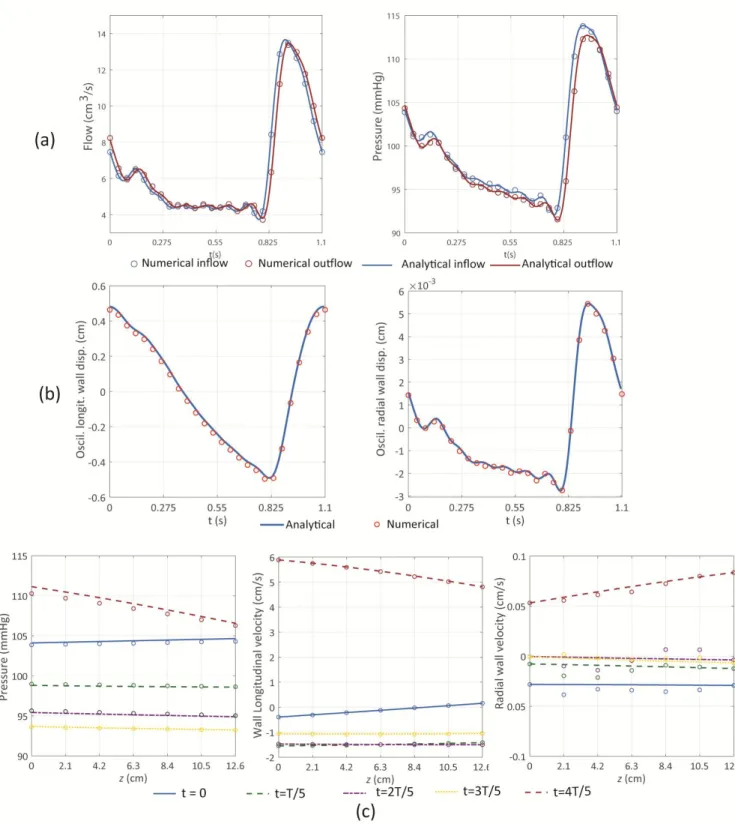
Flow and pressure waveforms: Figure 6(a)shows a comparison between analytical and numerical flow and pressure profiles at the inlet and outlet boundaries of the vessel. Pressure waveforms lag flow at both locations, a characteristic trait of hemodynamics in large vessels. The agreement between numerical and analytical solutions is excellent: the relative L2-norm error for outlet flow rate and pressure are 1.06% and 0.2%, respectively.

Figure 6. (a) Numerical versus analytical solution: flow and pressure at inlet and the outlet of the vessel; (b) Oscillatory parts of

wall longitudinal and radial displacements over time, at ; (c) Comparison between the analytical (lines) and numerical (circles) wall pressure (left), wall longitudinal velocity (middle), and radial velocity (right) along the vessel axis at

Figure 7 shows longitudinal and radial velocity profiles at the central cross-section of the vessel,

2 6.3

z L  cm, for different times of the cardiac cycle, for the numerical and analytical solutions. This location was chosen for being the farthest away from the boundaries, and therefore the least subject to the impact from the boundary conditions, which directly prescribe the velocity (inlet face) or impedance function (outlet face). Solutions are plotted along a line y  ( R R, ).

Longitudinal velocities: Figure 7 (left) shows the total analytical velocity, its oscillatory component and the numerical solution. Velocity profiles are shown to be periodic. Wall velocity oscillates around a zero mean, showing negative (backwards) and positive (forward) oscillating values thorough the cycle. The comparison between analytical and numerical total velocity profiles shows a good agreement, with a relative L2-norm error smaller than 6.7%.

Radial velocities: Figure 7 (right) shows a comparison between the analytical and numerical radial velocity profiles. For the fluid domain, the magnitude of the longitudinal velocities is ~ 30 cm/s and the radial velocities ~ 0.02 cm/s, a 1,500 ratio. For the wall velocities, this ratio is significantly smaller ~50, in agreement with Figure 3(a). There is a poor agreement between radial velocity profiles: relative L2-norm error is as large as 178% for t 2T / 5 and 47% for t T .

Wall displacements: Figure 6(b)shows a comparison between analytical and numerical oscillatory displacements in the longitudinal (left) and radial (right) directions at z L 26.3cm. The profiles show a good agreement, with relative L2-norm errors in the longitudinal and radial displacements of 5.6% and 3.8%, respectively.

Spatial distributions of wall pressure and velocity: Figure 6 (c) shows a comparison between analytical and numerical solutions for wall pressure, longitudinal and radial wall velocities along the vessel at different times. There is a good agreement for the wall pressure and longitudinal velocity (maximum relative L2-norm errors of 0.6% and 2.2%, respectively). The radial velocity displays good agreement for large velocity values, while for small values the discrepancy increases. This discrepancy is due to the small radial velocity values relative to the main longitudinal components.

Figure 7. Comparison between analytical and numerical solutions for longitudinal (left) and radial (right) velocity profiles

at the central section of the vessel at different times.

Pulse wave propagation: A wave propagation speed can be calculated as the ratio of vessel length and pulse transit time between the inlet and outlet waveforms using the foot-to-foot method 40. Using the numerical pressure waveforms, a wave speed of num 693

c  cm/s was obtained. This is a 4% difference from the wave speed obtained using the analytical waveforms canalyt 664 cm/s. By contrast, the Moens-Korteweg formula (Remark 6 in Appendix) produces an estimate for pulse wave velocity in an inviscid fluid of

0 702.26

c  cm/s. This estimate is larger than the previous values because of wave attenuation, present in the numerical and analytical waveforms, but absent in the Moens-Korteweg formula.

Linear behavior and thin wall assumptions: The analytical estimate for the scale parameter  defining the magnitude of the contribution of the non-linear advection to the total momentum was found to be smaller than 4%. This bound was confirmed by the numerical solution, which produced an upper bound for the scale parameter num _3.6%_.

Lastly, the maximum numerical radial wall deformation was _max R 0.0186, indeed small and

close to the theoretical estimate of num 2_{, eq. (17). These values therefore confirm the validity of the}

linear behavior (used just by Womersley’s theory), and the thin wall assumption (used by both Womersley’s solution and the CMM).

4

Discussion and Conclusions

The interaction between fluids and deformable structures is a key component of many multi-physics problems, especially in cardiovascular biomechanics. Modeling pulsatile blood flow within complex deformable vessels requires advanced FSI methods. To ensure credibility of these methods, it is important to perform verification (testing an implementation against an analytical solution) and validation (testing a theoretical model against experimentally acquired data) studies. Even though the CMM had been successfully used for numerous blood flow simulation studies for more than a decade 21,39,41, including validation against in vitro experimental data 42, and is a key component of the open-sourced software CRIMSON 35, a rigorous verification study of the method was still lacking.

In this paper, we verified the Coupled-Momentum Method FSI method for simulating blood flow in compliant vessels 20 by comparing it against a Womersley’s deformable wall solution 10,13, which can be regarded as the analytical solution for the CMM under the assumptions of idealized axisymmetric geometry, linear flow and wall responses. A key novelty of this work is the multi-frequency nature of the analytical solution, which allows for accurate representation of cardiovascular flow and pressure waveforms.

A thorough overview of Womersley’s analytical solution was first presented. This included a scale analysis to examine the validity of the main assumptions of the theory, namely linear flow and wall dynamics, long-wave and thin-wall approximations. Several non-dimensional parameters were identified: the parameter  w/ c 1 scales the non-linear fluid inertia terms. For the long-wave approximation to hold,  R / c 1.  scales the viscous stress terms, the pressure radial gradient, and the wall inertia component. The parameter   represents the ratio of a typical radial velocity to the wave speed. Lastly, the vessel wall is subject to the conditions:  / R 1 (small radial deformations) and

/ 1

h R  (thin membrane). Our analysis revealed that  is a critical scaling parameter, larger in magnitude than  and  (Erreur ! Source du renvoi introuvable.), and proportional to the radial deformation  / R (Remark 4). Material parameters for the application examples presented here were chosen such that all the conditions above are valid. In particular, maximum  at peak systole ~ 4%, thus ensuring consistency of the verification.

A verification study of the CMM was then presented. Since Womersley’s deformable wall solution is defined over a semi-infinite domain, a key component of this study was to prescribe a reflection-free outflow boundary condition via a characteristic impedance function. From the standpoint of solution verification, this outflow impedance presents a ‘softer’ condition than imposing pressure or velocity. The numerical solutions are therefore ‘less constrained’, thus enhancing the relevance of the verification study. The verification study considered an illustrative example of pulsatile blood flow in a straight cylindrical compliant vessel with parameters corresponding to a common carotid artery. Results demonstrated excellent agreement between numerical and analytical solutions for longitudinal velocities, wall displacements, pressure and flow waveforms, and pulse wave velocity. However, large discrepancies were observed between radial velocities. This can be partially explained by their small magnitudes and the small ratio relative to their longitudinal counterparts (a 1/1,500 ratio in fluid velocities, and 1/50 in wall velocities). Another factor potentially contributing to the discrepancy between radial velocity profiles is the lack of 2D axisymmetry of the 3D computational mesh and/or a bias from uniformly oriented structured mesh.

It is well known that the longitudinal component of vessel wall motion is not as large as that predicted by the analytical solution 13 used here. To address this shortcoming, Womersley incorporated a correction to the theory whereby longitudinal wall motion was constrained via added mass representing the

surrounding tissue 11. Computational FSI techniques can mimic such a constraint by introducing adequate surface traction forces, an approach also developed for the CMM 43.

The linear and axisymmetric assumptions of the analytical solution limit the scope of the verification study. Therefore, the CMM verification presented here does not take into account features such as advective inertial forces and complex geometries (noncircular cross-sections, tapering, curvatures, bifurcations, etc.). To address this limitation, in future studies we will compare the CMM against another 3D FSI solvers.

Acknowledgements

This work was supported by the National Institute of Health [grant U01 HL135842].

Supporting Information

We supplement our numerical results shown in Figure 6 (b),Figure 7 by movie files in the online

version. Video 1 demonstrates a 3D profile of the total fluid velocity as it changes over the cardiac cycle.

Video 2 shows 2D oscillations of the radial fluid velocity, revealing the lack of axisymmetry. Video 3 and Video 4 demonstrate pulsations of the total wall displacements and oscillatory radial wall displacements,

respectively.

Appendix

Derivation of the deformable wall Womersley’s solution for a linear system of governing equations,

Erreur ! Source du renvoi introuvable., is described next. A.1. Harmonic waves

Solutions to the linear system of governing equations can be obtained via superposition of harmonic waves. Separation of variables is assumed for each unknown, as well as periodicity in time with frequency  :

1( ) exp( ( )), 1( ) exp( ( )), 1( ) exp( ( ))

uu r  i tz ww r  i tz pp r  i tz , (31)

exp( ( )), exp( ( ))

K i t z N i t z

        . (32)

Here, K N,  are non-dimensional constants, independent of

r



, due to the fixed mean radial displacement assumption (eq. (12)). For convenience, the non-dimensional variable   r R  r and parameter 3/ 2

i 

  are introduced. Substituting u w p₁  , ₁, ₁ from eq. (31) into the fluid governing equations, Erreur ! Source du renvoi introuvable.(A), expressing variables in terms of  and using

2 2 i   , we obtain:

 

_{ }

_{ }

1 1 1 0, du _i u w d              (33)

 

 

_

_

_{ }

 

2 1 1 1 2 2 2 1 2 1 2 , d u du dp u i d d d





_





















         (34)