Design of multi-passage cooling systems for avionics applications

DESIGN OF MULTI-PASSAGE COOLING SYSTEMS FOR AVIONICS APPLICATIONS

by

David B. Vetter

Submitted to the Department of Mechanical

Engineering in Partial Fulfillment

Requirements for the Degrees

of the of

BACHELOR OF SCIENCE

and

MASTER OF SCIENCE

in Mechanical Engineering

at the

Massachusetts

Institute of Technology

June 1993

@Massachusetts

All rights reserved

Signature

Certified

of A

by

uthor

Signature redacted

Department of Mechanical Engineering

May 19, 1993

Signaiure

redacted

I-Signature

/11Professor Peter Griffith

redactedThesis

Supervisor

Accepted by

Graduate Committee

AUG 10 1993

1

DESIGN OF MULTI-PASSAGE COOLING SYSTEMS FOR AVIONICS APPLICATIONS

by

David B. Vetter

Submitted to the Department of Mechanical Engineering on May 19, 1993 in partial fulfillment of the requirements for the degrees of Bachelor of Science

and Master of Science in Mechanical Engineering

ABSTRACT

Models of multi-passage cooling systems, typical of those used use for cooling avionics, were created. The cooling systems considered

consist of manifolds which deliver fluid to several lateral flow elements in parallel. These models can optimize the selection of parameters and configuration in designing such cooling systems.

Tests were conducted to verify the reverse and parallel flow configuration models using 0.25 and 0.375 inch square flow channel

manifolds. In each test there were ten parallel flow passages tapped into the manifolds. Inlet flowrates were 2 gpm of coolant at approximately 630 F. Test configurations included 0.25 inch supply and return manifolds in both reverse and parallel flow configurations, 0.375 inch supply and return manifolds in both reverse and parallel flow configurations, and a 0.25 inch supply manifold and a 0.375 inch return manifold in a reverse flow configuration.

The 0.25 inch supply manifold and 0.375 inch return manifold in the reverse flow configuration provided the most constant lateral flow

distribution of all configurations tested.

Thesis Supervisor: Peter Griffith

TABLE OF CONTENTS

Abstract ... 2

1. Introduction... 4

2. Analysis... 7

2.1. Division Of System Into Flow Elem ents... 7

2.1.1. Dividing Tee... 7

2.1.2. Combining Tee... 8

2.1.3. Lateral Elem ent... 9

2.1.4. Straight Manifold Section... 1 1 2.2. M anifold System Solutions... 1 1 2.2.1. Dividing Solution... 1 1 2.2.2. Com bining Solution... 1 3 2.2.3. Reverse Flow Solution... 1 5 2.2.4. Parallel Flow Solution... 17

3. Test Setup... 1 9 4. Results... 27

4.1. Plenum ... 27

4.2. Straight M anifold Section... 28

4.3. 0.25 Inch Manifold Pairs... 28

4.4. 0.375 Inch Manifold Pairs... 34

4.5. 0.25 Inch Supply, 0.375 Inch Return... 39

5. Discussion... 42

5.1. O ptim izing Distribution Of Lateral Elem ent Flow ... 42

5.2. Incorporating Lateral Resistance Characteristics Into M odel... 45

5.3. Param eters Affecting Distribution... 46

5.3.1. Manifold Size... 46

5.3.2. Lateral Resistance... 46

5.3.3. Lateral Elem ent Spacing... 47

5.3.4. Temperature... 48

5.3.5. Inlet Flowrates... 48

6. Conclusions and Recom mendations... 50

Appendix A-Test Fixture Drawings... 54

Appendix B-Sam ple Spreadsheet... 69

1. INTRODUCTION

This thesis is an investigation of flow distribution in modular forced liquid cooled avionics equipment. Its purpose is to develop an accurate analytical tool for optimizing flow distribution in forced liquid cooled modular avionics. Often, avionics flow distribution systems are designed using simple rules of thumb or worse yet, by trial and error. No

references are readily available to assist the designer of such a system in a way which is practical and easy to understand. Articles found in various engineering journals approached similar flow distribution problems but

not in a way which is useful to the practicing avionics packaging engineer. This thesis will allow a competent engineer to calculate the flow

distribution in a particular system of interest.

Most radars have a beam that is steered by mechanically displacing the antenna. Efforts are currently underway to produce electronically scanned antennas. While this would create a much faster and more versatile antenna, it would also require much more power.

Currently, forced air flow systems are widely used in cooling radar power supply electronics. With the implementation of the electronically scanned antenna, a forced liquid cooling system is more suitable than the current airflow system considering the increased amount of power

dissipation required. In addition, there is also a need for liquid cooling in the antenna itself.

The antenna consists of hundreds of individual transmitting and receiving modules. Each of these modules must be cooled. A manifold system, such as those to be investigated in this paper, may be used to

distribute coolant to each module. As in all avionics hardware, weight and space considerations are critical.

The systems under consideration will implement a reverse or parallel flow manifold system that will deliver coolant to several heat exchangers in parallel (Fig. 1). Dividing and combining flow manifolds which are often implemented in air cooled systems will be examined but will not be tested.

Reverse Flow

Divivding Flow

Parallel Flow

Combining Flow

Liquid cooling systems will allow much greater heat dissipation than the airflow systems currently used for Hughes Radar Systems Group avionics. This approach should be applicable not only to the F/A-18 radar set but also to other radar programs and other applications that utilize forced liquid cooling with modular avionics.

2. ANALYSIS

2.1. DIVISION OF SYSTEM INTO FLOW ELEMENTS

In order to characterize flow and pressure distributions in the system, the system must be broken up into several types of flow

elements, each with its own flow equation. Pressure regain and pressure decrease coefficients are introduced to take into account flow

uncertainties and element coupling effects.

2.1.1. DIVIDING TEE

The first of such elements is the dividing tee (see Fig. 2).

2

-3

Figure 2.1 Dividing Flow Control Volume

This tee consists of a channel of uniform cross section and an opening in the wall of the channel through which flow is diverted from the main channel flow stream. A momentum equation balance can be used to determine pressure drop across the branch point:

-

The system will be solved for steady state conditions, so first term, the rate of accumulation of linear momentum, is zero. The remaining terms solved in the axial direction give:

JpV

V

dA

JpV1VldA1 +JpVnVidA

J

P

dA1

JP

dA

(Eq. 1.2)

or:

pV22A2-pV1 2A1+pV1V3A3 - P1A1 - P2A2 (Eq. 1.3)

The angle which the diverted flow exits the control volume through A₃ is unknown, so there exists an uncertainty in the amount of axial momentum flux across A3. A pressure regain coefficient, Yd, is used to account for

this uncertainty. Yd has been determined form experimental results experimentally for several geometries and flow conditions by Bajura2_.

Most of these values were around Yd = 0.8, but values ranged from approximately 0.7 to approximately 1.

Using this coefficient and the relationship Q=VA, Equation 1.3 can be rearranged to express the static pressure change across the dividing

branch as a function of discharge ratio, Q1/Q₃, entering dynamic head, rV₁2_{/2, and the regain coefficient, Yd:}

q3 Q3 pV12

P2-P1

=

4 2

1

---3

4

Figure 2.2. Combining Flow Control Volume

In a similar manner the equation relating pressure change across a combining tee can be found. The momentum equation applied to the combining tee at the branch point gives the equation:

Q₃ __3pV1

P2-P1 = 2 - p

- ) 2 (Eq. 1.5)

where Yc is a pressure decrease coefficient determined by the axial velocity of the lateral stream entering the combining flow channel.

Bajura2 found that yc varied with the diameter ratio, D3/D1. Values of yc

ranged from about -0.8 to about 0.2 over a diameter ratio range of 0.19 to 0.53.

2.1.3. LATERAL ELEMENT

The next flow element considered is the lateral element. The flow rate through the lateral is dependent on the lateral flow resistance and the pressure differential across the lateral. The lateral flow resistance

may consist of local losses, frictional losses, turning loss from the delivery manifold into the lateral, and turning loss from the lateral into the return manifold. The arithmetic average of pressures just upstream and just downstream of the branch points are used to determine the pressure differential across the lateral.1,2 The flow equation for the lateral is then:

P1+P2 P3+P4

2

2

[K

f(UD)

Ctd

+1]pV

_/2

_{(Eq. 1.6)}

1 2

3 4

Figrue 2.3. Lateral Element

where P1, P2, P3, and P4 are pressures at the locations indicated in figure

2.3 and the arrow indicates the direction of flow.

In this equation the losses are lumped together and termed Kiat, the lateral loss coefficient, where Kiat = [K+ f(UD) + Ctd + Ctc +1]. The lateral element pressure drops can sometimes be determined from heat exchanger or flow element specifications, although better results will be achieved if

the pressure drops are determined empirically for the flow rate range which will be used. A curve fit of the data can then be substituted for the

Kiat term in the above equation. Common curve fits are generally in a more complicated form than AP a V2. The effects of these different curve fit equations are discussed in the Discussion portion of the thesis.

2.1.4. STRAIGHT MANIFOLD SECTION

The final element of the manifold system to be characterized is the straight section of manifold flow channel between branch points.

Frictional losses in the channel are determined by the following equation:

P2-P1 = f 2 (Eq. 1.7)

Where L and D are the length and diameter of the straight section and V is the fluid velocity through the section. The pipe is assumed to be smooth and f is estimated by f=0.316 Re-0_.25 _{for turbulent flow and f = 64/Re for}

laminar flow. In the cases of laminar and turbulent flow, the friction factor, f, will vary along the combining or dividing manifold as velocities and hence Reynolds numbers change.

2.2. MANIFOLD SYSTEM SOLUTIONS 2.2.1. DIVIDING SOLUTION

The dividing flow manifold is often used in forced air cooling applications where the air is discharged to the atmosphere. In this type of system, a fan or blower pushes air through the manifold system.

In order to solve pressure and flow distributions for the system, a value for the flowrate through the last lateral(farthest from the inlet) must be assumed known. If flowrates downstream of the lateral element numbered 5 in the figure are known, then Q₅ can be found.

1 2 3 4

5 2, J 6

Figure 2.4. Dividing Flow Manifold

The pressure changes along the two paths shown in the figure are equal. The arrows indicate the direction of flow. Both paths represent pressure drop from the branch point of lateral element 5 to ambient pressure. The pressure at the branch point is taken to be the average of the pressures just upstream and just downstream of the branch point. The pressure change along the path through lateral 5 is simply the lateral 5 pressure drop. The pressure change along the other path involves

pressure changes at the two tees, frictional losses, and the lateral 6 pressure drop. Equating the pressure changes along the paths gives:

P1+P

-P1

-P

2

+(P

P

)

2

Inserting the flow element equations into this equation gives: pV52 105 Q5 pV12 (L PV22 Kiat5 2 = ~2Q1 (2 _{-Yd- ) 2} +f 2 1Q₆ Q₆ pV32 pV62 2 3 (2 -

Yd

P 1 P 1 2

Kiat5 2A2 +

2 2A2

[

1

1

2A2 Q 2 - ja2 Qs (Eq.1.10)

- f PQ 22 + (2 - Yd - ) Q32 - K _at _ P Q62 = 0

- 1D2 A 2

2Q-

Q2 are Q3 always equal in this equation. If the flowrate through the last

lateral element (farthest from the inlet) is known, then this rate is equal to Q2, Q3, and Q6. With these values known, the equation can be solved for 05.

Once the flowrate through the second to the last lateral, Q₅, is known the flowrate through the third to the last lateral can be found. With this, the next lateral flowrate can be found and so on. In this manner all flowrates can be found successively.

In order to determine flowrates for a given inlet flowrate, the flowrate through the last lateral element must estimated initially. The value can then be iterated until the desired inlet flowrate is reached.

Often in air cooled systems, air is pulled through the manifold by a fan. Ambient air is sucked into the system.

An equation for the combining flow manifold can found in much the same way as the dividing manifold. In this case the flowrate through the lateral element closest to the manifold outlet must be assumed known.

1 2

3 4 5 6

Figure 2.5. Combining Flow Manifold

Equating the pressure changes along the two paths give the equation:

P+P₄

2

(Eq.1. 11)

Substituting the flow element equations into this equation gives:

pV12 Kiat1 ₂ pV6 2 _1Q 2 Q2 pV52 - Kiat₆ 2 +2Q ₅ (2-Yd- _{) 2} 1Q1, Q1 pV32 + 2Q1 (2

-

Yd

Kiat1 2A2 -

Q

2A2 2j A-2 + 7

-+[ 2A Q4 + 2 -OsQ5 (Eq.1. 13)

- Klat _at62A ' 0 62 . _Q5Q(2- ) Qa .Q 52 = o

5 2A2 D A

As in the dividing manifold case, the lateral element flowrate farthest from the outlet in this case must initially be estimated. With this value the previous lateral element flowrate con be solved. All flowrates are solved successively. The estimate made for the last lateral element flowrate can b adjusted until inlet conditions are met.

2.2.3. REVERSE FLOW SOLUTION

In order to determine the flow rates through a lateral in the reverse flow manifold system the flowrates downstream (farther from the inlet) of the lateral must be known. The lateral flow rate to be solved can then be described as a function of the downstream flow conditions. The sum of pressure increases or losses around the loop shown below must be zero. This provides the following equation:

_1+P2 7+P8 P2-1 -I P - 3 2 2 + 2 -23 2 3 + P4 2 P9 + P₁₀ 2

P2

1 2 3 4

5 6

7 8 9 10

Figure 2.6. Reverse Flow Manifold

This equation is written in this form so that it can be expressed in terms of the element flow equations:

Klat 2 Q5 Q5 pV1 2

4-Q,(

)

q

Q

Q

PV7

2

Using continuity equations and the relationship Q = VA, this equation can be expressed as a quadratic equation in Q5:

[Kiat 2Aiat2 ₊

₍₁

52 +

{[(2- Yd) Ks -(2- Yc) Kr] Q6}

Q

-(2 -

-

)Y

82

]0

(Eq. 1.16)

where Ks and Kr represents A for the supply and return manifold channels respectively. Take Q₆ to be the last lateral element in the system (farthest from the inlet). In this quadratic equation, if Q2, Q3, Q6,

Q

estimated for Q6 then the second to the last lateral flowrate can be found.

With this flowrate the third to the last flowrate can be found as all downstream flow conditions(Q2, Q3, Q6, Q8, and Qq) are known. This

process can then be repeated for all lateral elements in the manifold system.

Generally, when designing a manifold flow distribution system , the engineer designs to certain inlet flow conditions - pressure and/or

flowrate - rather than to the flowrate in the last lateral. In order to use the quadratic solution to solve flowrates for a system with a specific inlet flowrate, the flowrate in the last lateral must be estimated and an initial solution performed. The last lateral flowrate should then be

iteratively adjusted until the sum of all lateral flowrates is equal to the desired inlet flow.

2.2.4. PARALLEL FLOW SOLUTION

The parallel flow manifold yields a similar quadratic equation to that from the reverse flow manifold. The parallel flow manifold can be

broken up into the same flow elements with the same equations as the reverse flow manifold. Tracing a path around the loop in figure 2.5 yields the following quadratic equation for the parallel flow case:

[Kiat 2Aiat2 ₊

₍₁

{[(2- Yd) Ks +(2-

Y7)

[ f KsQ22 + (2 - Yd - ) Ksa2 - Kia 2 t2 062

-(2 -

Y -

In this case, if Q₆ is taken to be the last lateral element, Q10 is equal to the inlet flow rate. Q₂ and 03 are still equal to Q6, but Q8 and Qg are now

the inlet flow minus Q₆. For Q5, all downstream conditions are known and the equation can be solved. Again once the last lateral element flow rate is known all flowrates can be found by progressively solving for previous laterals.

Either of the quadratic equations can be easily entered into a PC spreadsheet application. These equations, along with the flow element equations can be used to find the pressures and velocities at discrete points in the manifold system. The spreadsheet will then enable the user to quickly estimate the pressure profiles in the manifold channels and the flow distribution in the laterals. The spreadsheet also performs the

iterations necessary to determine the last lateral flowrate needed to meet inlet flow conditions.

3. TEST SETUP

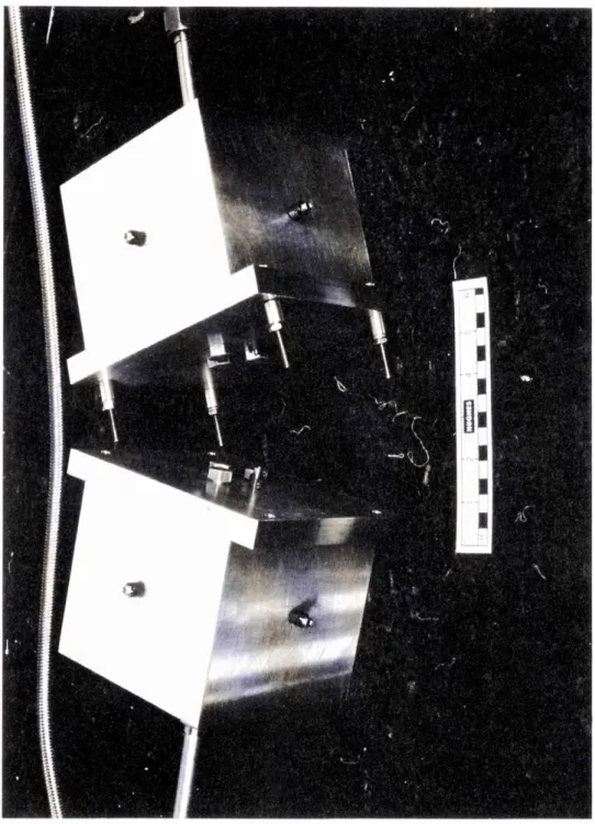
In order to verify the analytical method detailed above, several tests were conducted. In these tests two manifold systems were used. Each could be configured as a reverse flow or parallel flow system. Miniature quick disconnects were used as lateral elements. A schematic of the test setup and test fixtures used are shown in figures 3.1, .3.2, 3.3, and 3.4. Photographs of the test hardware are also provided in figures 3.5 and 3.6 and detailed drawings are

provided in Appendix A.

Pressure

Voltmeter I v Transducer

QD to be coupled with test fixture pressure tap QDs

7

Test

Coolanol Cart

Figure 3.1.

Test Setup

:ixt

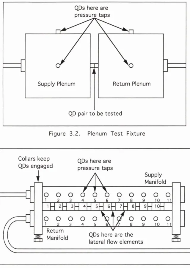
3.2.

Plenum Test Fixture

Collars keep

QDs engaged

4f

QDs here are

pressure taps

Return

Manifold

QDs here are the

lateral flow elements

Figure 3.3.

Reverse Flow Manifold Configuration Test Fixture

QDs here are

pressure taps

Supply Plenum

Return Plenum

QD pair to be tested

Figure

]

]

A

Manifold

1H

10H-0 10H-0 10H-0 10H-0 10H-0

0 0 0

Collars keep

QDs engaged

L

f

QDs here are

pressure taps

QDs here are the

lateral flow elements

Figure 3.4. Reverse Flow Manifold Configuration Test Fixture

Supply

A

Manifold

10-0 10-0 10-010-0

00

0 0

I

I 3!

I

I

I

01

I

I

I

Figure 3.6 Manifold Test Fixture. Shown Here in Reverse Flow Configuration

The lateral elements in the setup were miniature quick disconnects(QD's). These QD's consist of a male and a female half, which when mated provide a flow passage with consistent pressure drop characteristics. Lateral element locations are numbered one through ten in the Figures 3.3 and 3.4 above.

The combining and dividing flow manifold assemblies were machined from aluminum. One channel pair had a 0.25 inch square flow passage, and a second pair had a 0.375 inch square flow

passage. At each end of the flow channel assemblies, a connector or plug was installed to provide a flow inlet or outlet on the desired end. This allowed for both parallel flow and reverse flow

configurations.

Ten miniature QDs were installed in the assemblies at one inch intervals long the flow path. These QDs could then be mated to the QDs of another assembly to provide ten lateral elements. The QDs were spaced one inch apart. Because the QDs used were not locking QDs, a collar was constructed which held the manifold pairs

together. This ensured the male and female halves were coupled. QDs were also installed in the assembly on a side adjacent to the lateral QDs to provide pressure taps. These were located midway between the lateral elements. Manifold pressure tap locations are numbered one through eleven in Figures 3.3 and 3.4.

A pressure transducer was coupled with a QD which could be mated with the pressure tap QDs along the assemblies to obtain pressure readings. The transducer was wired to a voltmeter which provided the pressure values.

The total pressure drop through the lateral element was not just the pressure drop of the QD, but also the pressure drop across orifices in the side walls of the manifolds. A supply plenum and a return plenum with orifices and QD taps identical to those in the manifold side walls were constructed. The supply and return plenums each had a fluid inlet or outlet and two QD pressure taps, one on the top and one on a side of the reservoir. The two plenums could be connected so that the QDs to be tested were coupled. The pressure difference between the plenums was then the lateral

element pressure drop. The pressure transducer was used with this assembly to provide pressure values.

Coolanol, a coolant widely used in avionics, was the fluid used for the tests. The fluid flow was provided by a coolanol cart(pump). This cart could provide a range of pressures and flow rates. The cart had its own flowmeter and pressure gages.

A bypass of the test fixture was installed in the setup so that low flowrates through the test fixture could be obtained. The

amount of flow through the bypass was regulated with the valves located as shown in figure 3.1.

Flowrate through the test fixture was found using a turbine flowmeter downstream of the test fixture. The flowmeter was attached to a frequency counter. The frequency counter output was used with calibration data to determine the flowrates.

A thermocouple was located at the test fixture outlet so that fluid temperature could be determined. This data was necessary to find fluid characteristics and for flowmeter calibrations.

The first series of tests were performed using the supply and return plenums. Three separate pairs of QDs were tested in order to find the lateral element pressure drop. Flowrates at which the tests were conducted ranged from 0.097 gallons per minute to 0.322 gpm. Pressures were found using the transducer.

In order to verify the straight manifold section relationships, a single 0.25 inch manifold was tested. This manifold was not

coupled with the second of the pair. The coolanol inlet was attached to one end and the outlet to the other, so that there was a straight flow path. Pressures at each tap were measured for flowrates of 1 gpm and 2 gpm.

The manifold pairs were tested next. Each pair was tested in a parallel flow and a reverse flow configuration. All of these tests were conducted with an inlet flowrate of 2 gpm. Pressures at every pressure tap were measured and recorded. Pressures measurements midway between every lateral element, upstream of the first

lateral, and downstream of the last lateral were provided.

The final test was conducted using one 0.25 inch manifold and one 0.375 inch manifold. In this test, the manifolds were in the reverse flow configuration. The 0.25 inch manifold was

implemented as the supply manifold and the 0.375 inch manifold was the return manifold. This test was also conducted with an inlet flowrate of 2 gpm. Pressure measurements were recorded at all pressure tap locations.

4. RESULTS 4.1. PLENUM

The results of the plenum tests appear in the graph below:

PLENUM TEST DATA AND FITTED CURVE

0 041 LU Op W/ _ _ U 5i IAdd '4 0.1 0.2 0.3 FLOWRATE (GPM)

Figure 4.1. Plenum Test Data

Here the data points have been fitted to the curve AP = 31.27 Q2 + 5.32 Q.

This is the lateral flowrate relationship which is used in the manifold flow distribution equations developed previously. This relationship is not in the same form as the lateral element equation above, but it can still be used with the manifold flow distribution equations as described in the Discussion section of this paper.

" QD pair 1

o QD pair 2

* QD pair 3

P = 31.27*Q^2 + 5.32*0

4.2. STRAIGHT MANIFOLD SECTION

The tests conducted to find the frictional loses in a straight

manifold section determined that the losses were 0.33 psi and 1.2 psi for the 1 gpm and 2 gpm flowrates respectively. The 1 gpm flowrate resulted

in a Reynolds number of 1610. The calculated frictional loss for the ten inch section was 0.33 psi. The friction factor 64/Re was used in this laminar case. The calculated flowrate and Reynolds number for the 2 gpm flowrate were 3220 and 1.2 psi. In this case, the Blassius correlation was used. In both cases the actual pressure drops were higher than the calculated pressure drops. Part of this difference may be attributed to the pressure taps and lateral element taps in the manifold side walls. These irregularities probably caused additional losses, but these losses are taken into account in the regain and decrease coefficients in the tee flow element equations. Also both of the Reynolds numbers are close to the transition number for a flow channel. Reynolds numbers in this range tend to exhibit somewhat unpredictable behavior. Unfortunately, many of the Reynolds numbers which appear in the testing fell in or near this transition range. The dimensions and flowrates which yield these Reynolds numbers were selected because they are typical for existing prototype avionics systems. The discrepancies in calculated and actual frictional losses should not be a concern. A reasonable small error in the friction factor will have little effect on the results from the model.

4.3. 0.25 INCH MANIFOLD PAIRS

The results of two separate tests for the 0.25 inch manifold pair in a reverse flow configuration are plotted here along with expected values from the equation developed above. The spreadsheet used for these

calculations is included as an example in appendix B. The regain and decrease coefficients used to find expected values were Yd = 0.8 and Yc =

-0.7. Other equation constants were based on the test setup dimensions. Tap location number one is closest to the inlet and tap number eleven is farthest. 4.500 4.000

]__

p

PRESSURE TAP LOCATION

Figure 4.2. Analytical versus Experimental Data for 0.25 Inch Manifold, Reverse Flow

.1

JVLA

The pressure values in the plot are referenced to the return manifold outlet. The return manifold pressure at tap location 1 was subtracted from all other pressure values.

The flowrates through the lateral elements in the system are determined by the difference in supply manifold pressure and return manifold pressure at a specific point. For the 0.25 inch manifold pair in the reverse flow configuration this difference is significantly larger at the small pressure tap location numbers than at the larger tap numbers. This indicates that the flow elements near the inlet have higher flow rates than those farther downstream.

In the supply manifold two types of pressure changes are taking place. There are frictional pressure drops in the direction of flow, but pressure increases in the direction of flow at each lateral element

junction due to the diversion of flow. The frictional losses and pressure regains tend to negate each other so that the overall pressure gradient in the supply manifold is relatively small. In the return manifold there are two types of pressure changes which compound each other. Again there are frictional losses in the direction of flow, but at the junctions there are pressure losses rather than regain due to the combining flow.

Pressure gradients in the return manifold tend to be larger than those in the supply manifold. This can be seen in many of the graphs provided.

4 00 0 .A AA 3.500 -- .".SUPPLY EXPECTED 3.000 RETURN

o.

5EXPECTED

PRESSURE TAP LOCATION

Figure 4.3. Analytical versus Experimental Data for 0.25 Inch Manifold, Parallel Flow

The experimental and analytical data for the 0.25 inch manifold in a parallel flow configuration are plotted above. Unlike the reverse flow configuration, this configuration has larger lateral element flowrates at the locations farthest from the inlet. As can be seen in the graphs the supply manifold for both configurations have similar gradients; the

pressure increases by about 0.5 psi along the length of the manifold. The return manifolds' pressure gradients have nearly the same shape, but they are reversed. The return manifold in the reverse flow configuration has a pressure going from 0 to approximately 2 psi while the return manifold in

the parallel flow configuration has a pressure going from approximately 2 psi to 0 psi. The reverse flow configuration provides the flow

distribution than the parallel configuration because its supply and return manifold pressures are both increasing. This provides a more constant pressure difference between the manifolds, and thus a better flow

distribution. The parallel flow configuration has pressure increasing in the supply manifold at the same time it is decreasing in the return manifold. The pressure differences for each configuration are plotted below. U, C,, C', w cc 4 3.5 3 2.5 2 1 .5 1 0.5 0 * ~ 6

PRESSURE TAP LOCATION

1 11

Figure 4.4. Supply And Return Manifold Pressure Difference, 0.25 Inch Manifolds PARALLEL FLOW TEST, 1-5-93 -0--- PARALLEL FLOW TEST, 1-11-93 REVERSE FLOW TEST, 1-5-93 -0--- REVERSE FLOW TEST, 1-11-93

As can be seen in the above graph the pressure difference for the reverse flow manifolds is more constant than the parallel flow manifolds although neither would appear to provide what could be considered an even flow distribution.

The flow distributions determined in the analysis appear in the graph. Lateral element number one represents the element closest to the fluid inlet.

iU

LATERAL ELEMENT LOCATION

Figure 4.5. Analytical Flow Distributions, 0.25 Inch Manifolds

REVERSE FLOW _ _ PARALLEL

FLOW

The flowrates provided from the analysis further prove that the reverse flow configuration provides a more even flow through the lateral elements. Perfectly even flow distribution would have all lateral element flowrates 0.2 gpm. For the parallel flow configuration the lateral element flowrates ranged from 0.1534 to 0.2692 gpm. These values are 23 percent below and 35 percent above the average flowrate of 0.2 gpm. The reverse flow configuration flowrates ranged from 0.1731 to 0.2465 gpm, 13

percent below and 23 percent above the average flowrate. In most cases, an unexpected lack of coolant is the primary concern, but an excess of coolant may also cause problems for components that perform optimally in a particular temperature range.

4.4. 0.375 INCH MANIFOLD PAIRS

The 0.375 inch manifolds have much smaller pressure gradients in the supply and return manifolds than do the 0.25 inch manifolds. The pressure tap readings for the 0.375 inch manifold in the reverse flow and parallel flow configurations are plotted below along with their calculated values.

3 C,, C,, 2.5 2 1.5 1 0.5 0 A AA

1

----

. .

PRESSURE TAP LOCATION

Figure 4.6. Analytical versus Experimental Data for 0.375 Inch Manifold, Reverse Flow -- "-- - SUPPLY EXPECTED -- 0--- RETURN EXPECTED SUPPLY TEST, 1-5-93 RETURN TEST, 1-5-93 A SUPPLY TEST, 1-11-93 A RETURN TEST, 1-11-93 .-- 4-0

3

I-.

PRESSURE TAP LOCATION

Figure 4.7. Analytical versus Experimental Data for 0.375 Inch Manifold, Parallel Flow

The 0.375 inch manifold plotted pressure curves are similar to the 0.25 inch manifolds pressure curves, but the pressure gradients are much smaller in the 0.375 inch cases. Again the pressure rises in the supply

manifold farther from the inlet in both cases. Pressure decreases in the direction of flow for reverse and parallel flow in the return manifold.

As in the 0.25 inch manifold pairs the pressure differences between manifolds is more consistent in the reverse flow case. These pressure differences are graphed below.

3.000 2.000 1.500 1.000 0.500 0.000 I I 1 6 11

PRESSURE TAP LOCATION

Figure 4.8. Supply And Return Manifold Pressure Difference, 0.375 Inch Manifolds

The average pressure change along the length of the manifold for the two reverse flow tests was 0.315 psi. For the two parallel flow tests the average pressure change was 0.555 psi. The reverse flow configuration will give a more even flow distribution for these test conditions. The flow distributions for the 0.375 inch manifolds in the reverse and parallel flow configurations from the model are shown below.

PARALLEL FLOW TEST, 1-5-93 -~- PARALLEL FLOW TEST, 1-11-93 - - REVERSE FLOW TEST, 1-5-93 0- REVERSE FLOW TEST, 1-11-93

O 25 0.2 .0 .15

W

Figure 4.9. Analytical Flow Distributions, 0.375 Inch Manifolds

For the 0.375 inch manifolds, the reverse flow configuration has a just slightly better flow distribution than the parallel flow configuration. The

lateral element flowrates range from 0.1943 to 0.2097 gpm for the reverse flow and from 0.1896 to 0.2140 gpm for the parallel flow

manifolds. For the reverse flow, this range is from 3 percent below to 5 percent above the 0.2 gpm average lateral element flowrate. This is 5 percent below to 7 percent above the average flowrate. For avionics applications, a cooling system which provides at worst 5 percent less flow than is expected to a particular lateral element certainly acceptable.

-- REVERSE FLOW

-- PARALLEL

4.5. 0.25 INCH SUPPLY, 0.375 INCH RETURN

The last test was run with a 0.25 inch supply manifold and a 0.375 inch return manifold. Inlet flowrate was again 2 gpm. The pressures at the taps in each manifold are plotted below. The average pressures for the two 0.375 inch manifold reverse flow tests are also plotted here for comparison.

3

00n

1....

PRESSURE TAP LOCATION

Figure 4.10. Experimental Data for 0.25 Inch Supply/0.375 Inch Return Manifolds and 0.375 Inch Manifolds, Parallel Flow

From the graph, it becomes apparent that the system with the smaller supply manifold will have flow distribution similar to that in the system

--- _{0.25 SUPPLY} 3 0.375 RETURN -- *-- SUPPLY TEST AVERAGE 0 RETURN TEST AVERAGE

with the 0.375 inch supply manifold. The pressure differences between supply and return manifolds for the two cases are graphed here:

-~ U -U U -. 3 2.5 2 1.5 1 0.5 0

Figure 4.11. Supply And Return Manifold Pressure Difference, 0.25 Inch Supply/0.375 Inch Return Manifolds and 0.375 Inch Manifolds

The difference changes by nearly the same amount along the length of the manifolds for both cases. _{The flowrates, analytically determined using} the model, are compared in the graph below.

40 0--F5 cc, Cn wn W. 6

PRESSURE TAP LOCATION

i -- "- 0.25 SUPPLY/0.375 RETURN 3---- 0.375 SUPPLY/0.375 RETURN

I

1

0.2500 0.2000 0.1500 0.1000 0 -j U. 0.0500 n n0nn I I I 1 4 7 10

LATERAL ELEMENT LOCATION

Figure 4.12. Analytical Flow Distributions, 0.25 Inch Supply/0.375 Inch Return Manifolds and 0.375 Inch Manifolds

Here the 0.25 inch supply manifold with the 0.375 inch return manifold provides a better flow distribution through each of the laterals than the 0.375 inch supply and return manifolds. The smaller supply manifold system provides a lateral flowrate range of 0.1965 to 0.2042. These flowrates are about 2 percent below and above the average 0.2 gpm flowrate. 0.375 SUPPLY/0.375 RETURN --- _0.25 SUPPLY/0.375 RETURN

5. DISCUSSION

5.1. OPTIMIZING DISTRIBUTION OF LATERAL ELEMENT FLOW

It is evident from the manifold pressure profile graphs

presented that pressure undergoes greater changes along the return manifolds than the supply manifolds. As stated before, the supply manifold undergoes two opposing types of pressure change. The pressure drops due to frictional losses while it increases at the branch points due to the dividing of the flow. The return manifold undergoes two compounding pressure changes. The frictional losses are still present, but in this case there is a pressure decrease at the branch points due to the combining of the flow.

In the 0.25 inch manifold cases, for both configurations the pressure regain effects dominate frictional losses in the supply manifold. This is what causes the pressure to rise along the supply manifold in these cases. In the return manifold, the compounding pressure decreases across the tees and frictional losses cause a relatively large pressure drop in the direction of flow.

In the reverse flow case, because the flow directions in the two manifolds oppose each other, the pressures in both manifolds increase at the pressure taps with increasing pressure tap numbers. The parallel flow configuration has manifold flows in the same direction. This results in an increasing pressure in the supply manifold with increasing pressure tap number and a decreasing pressure in the return manifolds with increasing pressure tap number.

The configuration which provides the better flow distribution will be determined by the pressure regain effects' dominance over the

frictional losses. The pressure profiles for the supply and return manifolds are more closely matched in the reverse flow configuration used here. This provides the better flow distribution. But a case where the frictional losses dominate the regain effects, the pressure profiles for the supply and return manifolds will be more closely matched in the parallel flow configuration.

The same type of situation exists in the 0.375 inch manifolds set. In the reverse flow configuration the pressure characteristics for the supply and return are more closely matched yielding a better flow distribution. The pressure curves for the 0.375 inch manifolds in the reverse and parallel configurations are much more constant than in the 0.25 inch manifolds. The velocities of the fluid through the 0.375 inch manifold flow channels will be much smaller than the velocities present in the 0.25 inch manifold channels. The relationships for pressure regain or decrease across a tee and for frictional losses all involve a V₁2 term. The

relationships are not strictly AP a V₁2 because other terms in the equations involve V1, but the pressure changes are very sensitive to changes in fluid velocity in the manifolds. The larger manifolds are approaching plenum behavior.

This brings up the first strategy for creating an even flow distribution system. An ideal situation would have perfectly even

pressures in both the supply and return manifolds. This would provide an equal pressure differential across all lateral elements, and thus an even flow distribution. In order to approach this condition the pressure

relative to the lateral element pressure drops. A cooling system of this type guarantees an even flow distribution, but is not necessarily the best system when weight and space considerations are crucial.

This brings about another strategy for achieving nearly even flow distribution. With the 0.25 inch manifold pairs the pressure changes were larger along the lengths of both the supply and return manifolds than the pressure changes in the 0.375 inch manifolds. In all of these cases the return manifold pressure changes were much larger those in the supply manifold. In order to even out flow distribution the shapes of the

pressure profiles in both the supply and return manifolds can be made to match each other as closely as possibly. From the 0.25 and 0.375 inch manifold tests it could be seen that a 0.25 inch supply and a 0.375 inch return manifold in a reverse flow configuration would provide the closest matched pressure profiles.

The last of the tests was conducted with such a configuration. It provided a slightly better flow distribution than the 0.375 inch supply and return manifolds. The main advantages of this system are that it saves space in that the supply flow channel is smaller and with the smaller channel, less fluid will be in the system saving weight.

Similar strategies may be employed for the combining and dividing flow manifolds that are often used in airflow systems. A nearly constant

pressure may be achieved if lateral pressures are large relative to manifold pressure changes. In the case of a dividing manifold, a fairly even distribution may be obtained with a relatively small manifold area by

balancing the effects of the frictional losses and the pressure regain. Balancing the effects of the frictional losses and the pressure regain in the supply manifold can also be an effective strategy in

acheiving a uniform flow in reverse and parallel flow systems. If a large enough return plenum is used to insure nearly constant pressure in the return manifold then balancing pressure gains and losses in the supply manifold will provide an even flow distribution.

One method often used to provide an even flow distribution is a tapered manifold. A taper could be created by placing a shaped

insert into the a manifold. This will cause fluid velocities to increase as the flow channel becomes smaller. Flowrate is equalized as fluid is lost through the laterals and flow area

decreases. Tapered manifolds are not examined in this paper, but the model developed could easily be modified to take into account the taper. Because the model determines pressures and flowrate at discrete points, some approximations will have to be made. The

model should give a reasonable estimate of flow distribution for a tapered manifold.

5.2. INCORPORATING LATERAL RESISTANCE CHARACTERISTICS INTO MODEL

Often flow elements such as heat exchangers or QDs are characterized by pressure drop data that has been fit to a curve. Second order polynomial curve fits lend themselves easily to the analysis. When a polynomial is used in the manifold model the flow solution equations remain quadratics which can be easily solved. The lateral elements used in the tests here had pressure drops

into the quadratic as Kiat and 5.32 is added to the second, or B, term of the equation.

Sometimes these curve fit equations do not have exponents that are whole. AP = AQB is frequently used to characterize a flow element. The exponent B will usually vary between one and two. In the flow model these equations do not yield quadratics but rather flow equations that must be solved iteratively. If this is the case

Kiat becomes zero and another term, AQ5B, must be added to the

equation where Q5 is being solved.

5.3. PARAMETERS AFFECTING DISTRIBUTION 5.3.1. MANIFOLD SIZE

Manifold delivery and return channel cross-sectional areas are perhaps the most important considerations when designing a

manifold system. Space, weight and performance of the manifold system must be considered. This is evident from the explanations above. Large manifolds guarantee even flow distribution, but smaller manifolds may be optimal.

5.3.2. LATERAL RESISTANCE

Lateral elements used in a manifold system for avionics are usually a heat exchanger module. The element may also include a coupler such as a quick disconnect. For an even flow distribution it is sometimes advantageous to have a lateral resistance that is large

relative to the losses in the manifold headers. This may be achieved by orificing the elements, but most of the pressure should occur where the heat transfer is taking place, in heat exchanger for example, so that dissipative potential is maximized.

Cases often exist where a predetermined uneven flow

distribution is desired. This condition will be fairly easy to obtain provided lateral pressure drops are large compared to those in the manifold. When this is true, the pressure along the manifold may be considered constant and adjustment of lateral flow may be

performed by assuming a constant pressure source.

Where overall system pressure drop is crucial, a small lateral element flow resistance may be desired. This is a case where the supply and return pressure profiles should be matched for a reverse flow system. For a dividing flow manifold the pressure regain will be balanced with the frictional losses.

5.3.3. LATERAL ELEMENT SPACING

Lateral element spacing will have an effect on the frictional losses in the manifolds. Clearly greater lateral element spacing will result in greater frictional losses in the manifold. If a constant pressure is desired in a manifold, smaller lateral element spacing is advantageous. Where a balance of pressure regains and frictional losses is necessary the

lateral element spacing becomes an important consideration. It is also important where pressure profiles are being matched.

Lateral element spacing may have an effect on flow distribution in that closely spaced laterals may experience coupling effects. These can

be accounted for in the regain and decrease coefficients but empirical data for these coefficients is somewhat sparse.

5.3.4. TEMPERATURE

Temperature of the fluid in the cooling system is an important, particularly where it not constant throughout the system. The tests described herein included no heat sources. Of course this will not be true of an actual system. Temperature will affect the viscosity and density of the fluid used. In the manifold models, one set of characteristics for a certain fluid temperature may be used in the supply manifold equations while another set for another temperature may be used for the return

manifold equations. In the lateral elements where the temperature change is taking place, yet another set of fluid characteristics may have to be implemented.

It should be kept in mind that a system which performs acceptably with a certain fluid may not perform adequately for another fluid or the same fluid at another temperature.

5.3.5. INLET FLOWRATES

A system which provides a uniform flow distribution at a particular flowrate will not necessarily provide an even distribution at other

flowrates. The pressures in the system flow elements will not all change at the same rate with changes in flow rates. Also, flow through the

vice versa. If this occurs, the pressure drop characteristics of the elements will certainly change.

6. CONCLUSIONS AND RECOMMENDATIONS

The model developed and presented here seems to very closely

predict pressures and flow distributions in manifold systems. This model should be a useful tool to an engineer in designing a multi-passage cooling system that utilizes manifolds. Too often, cooling systems are designed first and then "flow balanced" later by adding orifices or by some other

method. Many systems have been designed under the assumption that the manifold will act as plenum providing a constant pressure when, in fact, this is not the case.

The model will be able to identify cases in which nearly constant manifold pressures exist. Where there are not constant pressures, the model will help to determine parameters which provide an even lateral element flow distribution, or if desired, a particular uneven distribution.

In order to guarantee an even floW distribution, relatively large manifold diameters should be used. Large diameter manifolds will have small pressure changes relative to lateral element pressure changes. Supply and return manifolds will act as plenums in this case.

Often manifold diameters are limited and manifolds are not able to provide a constant pressure. When pressure regain in a supply manifold dominates frictional losses, as is the case in the manifolds examined here, a reverse flow configuration provides a better flow distribution than a parallel flow configuration. In the reverse flow configuration, the

pressures in both manifolds increase farther from the inlet. This matches the shapes of the manifold pressure curves.

The frictional losses in a supply manifold may dominate the

lateral spacing was increased. The parallel flow configuration provides a more even flow distribution than the reverse flow configuration in this case. With the parallel flow configuration, the pressures in both

manifolds decrease farther from the inlet providing better matched manifold pressure curves.

The manifold models developed provide a flexible tool to aid in designing a manifold flow system. It should allow an engineer to

determine the optimal configuration and parameters to obtain a desired flow distribution.

7. REFERENCES

1. Acrivos, A., Babcock, B. D. , and Pigford, R. L., "Flow Distribution in Manifolds," Chemical Engineering Science, Vol. 10, No. 1/2, 1959, pp. 112-124.

2. Bajura, R. A. , "A Model for Flow Distribution in Manifolds," Journal of Engineering for Power, Transactions of the ASME, Vol. 93, 1971,

pp. 7-12.

3. Bajura, R. A. , Jones, E. H., "Flow distribution manifolds," Journal of

Fluids Engineering, Transactions of the ASME, Vol. 98, 1976, pp.

654-666.

4. Dow, W. M., "The Uniform Distribution of a Fluid Flowing Through a Perforated Pipe," Journal of Applied Mechanics, Transactions of the

ASME, Vol. 72, Dec, 1950, pp. 431-438.

5. Fox, R. W. and McDonald, A. T., Introduction to Fluid Mechanics, John Wiley & Sons, Inc., 1978.

6. Gerhart, P. M. and Gross, R. J., Fundamentals of Fluid Mechanics, Addison-Wesley Publishing Company, 1985.

7. Haerter, J. H., "Flow Distribution and Pressure Change Along Slotted or Branched Ducts," ASHRAE Journal, Vol. 5, Jan. 1963, pp. 47-59. 8. Idelchick, I. E., Handbook of Hydraulic Resistance, Hemisphere

Publishing Company, 1986.

9. McNown, J. S., "Mechanics of Manifold Flow," Transactions of the

ASCE, Vol. 119, 1954, pp. 1103-1142.

10. Ruus, E., "Head Losses in Wyes and Manifolds," Journal of the

Hydraulics Division, ASCE, Vol. 3, Mar. 1970, pp. 593-608.

11. Aero-space Applied Thermodynamics Manual, Society of Automotive Engineers, Inc., 1962.

12. Arvidson, John M. and Brennan, James A., ASRDI Oxygen Technology

Survey Volume VIII: Pressure Measurement, Scientific and

13. Miller, Richard W., Flow Measurement Engineering Handbook, McGraw-Hill Publishing Company, New York, 1989.

Appendix A

5.25 z Supply QD (p/n 966078-5C) Pressure Tap QD (p/n AE88733A) .5 - -Pressure Tap QD (p/n AE88733A) Orfmmmmm-Supply Plenum .625

Notes:

'EU M - L n.aL-J

s-X

@ 2

- ---

Mini-QD Pressure Drop Test Fixture Set

Pressure Tap QD (p/n AE88733A)

Return Plenum

Face Plate,

Bond Face Plate to assembly using devcon

adhesive or equivalent

QD

2 1/2" 2" 5 1/4"

rEDIJIL

-T

-- 7

0

I3

13

4 3/4" 5/8" 2"

0

0

r

0

0

I

5/8"

2" 5 1/4"

-h-2"

2 1/2"

num

3

0

2 1/2"

0

I

I

7

i

If

JILL

1

EL

EL

R1

0

0)

0

F

2"

0

0

I

~1

-~1

I-EL

EL

0)

Aeroquip Mini QD (p/n AE88733A) D -Dimension "D" Supply Plunum Flow Test QDs S1 S2 S3 S4 0.0625 0.125 0.250 0.250 Aeroquip Mini QD (p/n AE88743A) DI Dimension "D" Return Plunum Flow Test QDs R1 R2 R3 R4 0.0625 0.125 0.250 0.0625 Aeroquip Mini QD (p/n AE88733A) D Dimension "D" Pressure Tap QDs 0.0625 Male QD (p/n 966078-5C)

IEEE

ID

* All ther dimensions as in SK921106M3,

Collar (2 rqd)

L

7

1"

w I

SECTION VIEW TWO-PIECE MALE MANIFOLD

ASSEMBLY

MALE MANIFOLD ASSEMBLY

L~i

_L8i

FEMALE MINIATURE QD: 2 PLCS PORT DIMENSIONS PER

AEROQUIP DWG AE88733A FEMALE PLUG .3125-24UNF-3A .125 MAX THD SI I SECTION VIEW TWO-PIECE FEMALE MANIFOLD ASSEMBLY .25 x .25 F-LOW CHANNEL

f1

FEMALE

BOND TO MAIN ASSEMBLY USING DEVCON ADHESIVE

MANIFOLD ASSEMBLY

HUGHES P/N 966078-5C MALE QD(4 REQD) END FITTING PER MS 33656E8