Design of cavitating propeller blades in non-uniform flow by numerical optimization

(1)

Design of Cavitating Propeller Blades in

Non-Uniform Flow by Numerical Optimization

by

SHIGENORI MISHIMA

B.S., The University of Tokyo (1986)

M.S., The University of Tokyo (1988)

Submitted to the Department of Ocean Engineering

in partial fulfillment of the requirements for the degree of

Doctor of Philosophy

at the

MASSACHUSETTS INSTITUTE OF TECHNOLOGY

September 1996

@

Massachusetts Institute of Technology 1996. All rights reserved.

Author ...

... ...

Department of Ocean Engineering

June 30, 1996

Certified by...

Department of Civil

. . . . . . . . . .. ... .

Spyros A. Kinnas

Assistant Professor

Engineering, The University of Texas at Austin

Thesis Supervisor

Accepted by ...

...

.-. ... ! ...

A. Douglas Carmichael

Chairman, Departmental Committee on Graduate Students

:••, •,:. ,-...,i:?·['--~'::" ir'S ,'S : J .

FEB I. 0 1997

UBRARIES

(2)

Design of Cavitating Propeller Blades in Non-Uniform

Flow by Numerical Optimization

by

SHIGENORI MISHIMA

Submitted to the Department of Ocean Engineering on June 30, 1996, in partial fulfillment of the

requirements for the degree of Doctor of Philosophy

Abstract

High-speed propulsor blades often experience moderate to substantial amounts of unsteady cavitation, and up to now have been designed via design methods for non-cavitating blades combined with methods for the analysis of non-cavitating flows in a trial-and-error manner.

In this thesis a numerical non-linear optimization algorithm is developed for the

automated, systematic design of cavitating blades. The objective and constraint

func-tions in the optimization process are expressed in terms of the design variables via linear approximations of the results from an existing lifting-surface analysis method, in the first stage of the algorithm, and quadratic approximations in the final stage. In this way the number of required geometries to be analyzed and the associated computational effort are minimized. The developed methodology is implemented in a modular manner so that future improvements in the modeling of cavitating flows can be readily incorporated. The proposed algorithm is validated with several known non-linear optimization test problems.

The method is first applied to the design of efficient two-dimensional partially and supercavitating hydrofoil sections and the results are compared to those from a previously developed optimization procedure.

Then, the method is applied to the design of propeller blades in uniform flow. The blade mean camber surface is defined via a cubic B-spline polygon net in order to facilitate the handling of the geometry, and to reduce the number of the design parameters. Non-cavitating blade geometries designed by the present method are directly compared to those designed via an existing lifting-line/lifting-surface design approach.

Finally, the optimization algorithm is applied to the design of cavitating blades in

non-uniform flow. The objective of the design is to obtain maximum propeller

effi-ciency for given conditions by allowing controlled amounts of sheet cavitation. Several constraints on the unsteady cavity characteristics, such as the area of cavity planform and the amplitudes of the cavity volume velocity harmonics, are incorporated in the optimization technique. The effect of the constraints on the efficiency of the propeller

(3)

design is demonstrated with various test cases.

Thesis Supervisor: Spyros A. Kinnas Title: Assistant Professor

(4)

Acknowledgments

There are a lot of contributions from many people to this thesis work. I first would like to express my greatest possible gratitude to my thesis supervisor, Professor Spy-ros Kinnas, at the University of Texas at Austin. He has always been encouraging me and giving me invaluable advices in every situation, even on weekends. I got several pieces of email every week from him and I knew he cared about my work. This pushed me to keep working hard. His contribution is so large that I almost feel as if he were a co-author of this thesis.

I would also like to thank my "step" supervisor at MIT, Professor Jake Kerwin, for his insightful and friendly advices on both good (rarely) and bad (mostly) results. He made comments always in a humorous way. I sometimes didn't realize the funny point until Todd Taylor explained it for me.

Professor Dimitris Bertsimas of the Sloan School of Management accepted to be-come a member of my thesis committee as an expert in optimization. He attended all the committee meetings and gave many useful comments from an optimization point of view, which I would have missed without him.

Dr. Ki-Han Kim of DTMB traveled all the way from Washington D.C. sometimes via Minneapolis to MIT and provided many practical suggestions, which I believe made this thesis more valuable.

I was really lucky to get to know smart Propnut members: Dr. Dave Keenan, Dr. Charlie Mazel, Dr. Ching-Yeh Hsin, Dr. Neal Fine, Dr. Mike Hughes, Dr. Tatsuro Kudo, Ms. Beth Lurie, Mr. Todd Taylor, Mr. Scott Black, Mr. Bill Milewski, Mr. Cedric Savineau, Mr. Wes Brewer, Dr. Bill Ramsey, Mr. Rich Kimball, Mr. Gerard Mchugh, Ms. Dianne Egnor, and Ms. Barbara Smith. Weekly group meetings were very helpful to get useful hints in my own research and to know other researches that were going on.

Bill Milewski took time to review my thesis draft and gave me good suggestions on it.

(5)

lunch.

Mr. Tatsuo Mori and Mr. Hideki Shimizu deserve credit for their friendship with me.

I would like to thank my former supervisors at the University of Tokyo, Professors Koichiro Yoshida, Hiroharu Kato, and Hideyuki Suzuki for their encouragements.

Professor Toshikazu Murakami of Tokai University is the person who made me consider studying at MIT, without whom I wouldn't even have started hydrodynam-ics research.

Special thanks go to my host family, Dr. and Mrs. Seigo Matsuda, who made my stay in Boston always much easier and more enjoyable.

Finally I would like to thank my wife, Naomi, for everything. I owe too much to her.

Much of the computation was performed remotely on "cavity", a DEC Alpha 600(5/266) computer of the Ocean Engineering Group in the Department of Civil Engineering at the University of Texas at Austin.

This research was supported by an international consortium of the following com-panies and research centers: Daewoo Heavy Industries Ltd., David Taylor Model Basin, El Pardo Model Basin, Hamburg Ship Model Basin, Hyundai Heavy Indus-tries Co., Ltd., Ishikawajima-Harima Heavy IndusIndus-tries Co., Ltd., KaMeWa AB, Mer-cury Marine, Michigan Wheel Corporation, Outboard Marine Corporation, Rolla SP Propellers SA, Sulzer-Escher Wyss GmbH, Ulstein Propeller AS, Volvo-Penta of the Americas, and Widrtsili Propulsion

Financial support for my stay at MIT was provided by the Technical Research & Development Institute, Japan Defense Agency.

(6)

6.3.3 Effect of Initial Blade Geometry . . . . 6.3.4 Torque-Constrained Design . . . . 78 . . . . 78 . . . . 82 . . . . . 83 . . . . . 88 . . . . 96 99 . . . . 99 . . . . 102 . . . . 102 . . . . 102 . . . . . 109 . . . . 109 . . . . 111 . . . . . 113 . . . . . 124 7 Conclusions and Recommendations

7.1 C onclusions . . . . 52 58 59 60 66 68 71 71 72 128 128

(8)

7.2 Recommendations ... ... 130

A One-Dimensional Line Search Method 133

B Data for the Test Problem 136

C Determination of Parametric Spacing for the Blade Geometry 138

(9)

List of Figures

2-1 Convergence history of the present method for test problem No. 2-3 . 36

3-1 Wake model used in HPUF-3A ... 42 3-2 Coordinate systems and geometrical notations in HPUF-3A, adapted

from [25] . . . .. . 44 3-3 Radial distribution of skew and rake, adapted from [35] ... 45 3-4 Construction of blade section from mean camber line and thickness form 46 3-5 Cubic B-spline basis (k = 4) : N, = 7 ... 49 3-6 Cubic B-spline curve : N,= 7 ... 50 3-7 Cubic B-spline surface. 4 x 4 vertex polygon net is shown together

with the 10 x 9 grid utilized in HPUF-3A ... 51 3-8 Chordwise and radial vortex lattice spacing from half-cosine and

uni-form spacing in u and w. The spacing required by HPUF-3A with 20 x 9 panels is also shown with dashed lines. . ... 53 3-9 Chordwise and radial vortex lattice spacing from iteratively determined

u and w. Notice that the vortex lattice is placed according to HPUF-3A 's schem e .. . . . . 54 3-10 Original N4381 blade geometry and the geometries defined by 4 x 4

and 7 x 7 B-spline vertices ... 55 3-11 4 x 4 and 7 x 7 B-spline vertices and contour plots of the error

distri-bution over the blade from the original blade, N4381. . ... 56 3-12 Forces and cavity volumes for original N4381 blade and 4 x 4 and 7 x 7

(10)

4-1 Flow chart of CAVOPT-3D ... 64

4-2 Flow chart of CAVOPT-3D, continued . ... 65 4-3 Construction of B-spline polygon net for initial propeller geometry . . 66 4-4 Design variables and B-spline vertices movement . ... 69 4-5 Initial B-spline polygon vertices, design variables, and vertex

move-m ent (4 x 4 vertices) ... 70 4-6 Contour plots of f () = (x - 1)4 + (x1- 1)2 2 • (X2 - 2)2 and quadratic

approximation of f(x) , top : f () , middle: quadratic approximation of f (x) (present algorithm) , bottom: quadratic approximation of f (x) (without x removal : converges to a wrong answer !) . ... 73 4-7 Convergence history of the variables and the function f(x) = (x1

-1)4 ₊ _(X

1 - 1)2x2 (x2 - 2)2 , top : present method (xl, x2)

(1.0, 2.0), f(x) = 0.0, bottom: without x removal ( 1, 2) = (0.89, 1.40), f(x) =

0.379 . . . .. .. . 74 4-8 Convergence history of design variables and function values for test

problem No. 4-1 ... 76 4-9 Convergence history of design variables and function values for test

problem No. 4-2 . ... ... ... .. .. ... . .. . 77

5-1 A partially cavitating hydrofoil ... .. 79 5-2 A supercavitating hydrofoil. ... 80 5-3 Optimum supercavitating foil geometry and corresponding pressure

distribution : CLo = 0.303, uo = 0.2, Re = 6.3 x 106 . ... 86 5-4 Different initial foil geometry guesses lead to the same optimum solution 87 5-5 Effect of A in the finite difference scheme for the initial linear

approx-imation of the functions on the required number of analysis runs and the solution : 6 = 0.02, e = 1 x 10-3 : Partially cavitating hydrofoil . 90 5-6 Effect of A in the finite difference scheme for the initial linear

approx-imation of the functions on the required number of analysis runs and the solution : 6 = 0.02, e = 1 x 10- : Supercavitating hydrofoil . . . . 91

(11)

5-7 Effect of the maximum movement of the variables, 6, on the required number of analysis runs and the solution : A = 0.05, e = 1 x 10- 3 _:

Partially cavitating hydrofoil ... .. 92 5-8 Effect of the maximum movement of the variables, 6, on the required

number of analysis runs and the solution : A = 0.05, = 1 x 10- 3 :

Supercavitating hydrofoil ... .. 93 5-9 Effect of the tolerance for convergence, e, on the required number of

analysis runs and the solution: A = 0.05, 6 = 0.02 : Partially cavitating hydrofoil . . . . . . . .. .. 94 5-10 Effect of the tolerance for convergence, e, on the required number of

analysis runs and the solution : A = 0.05, 6 = 0.02 : Supercavitating hydrofoil . . . . . . . .. .. 95 5-11 Inviscid optimum partially cavitating foil geometry and corresponding

pressure distribution (Re = 5.6 x 106) . ... ... 97 5-12 Viscous optimum partially cavitating foil geometry and corresponding

pressure distribution (Re = 5.6 x 106) . ... 98

6-1 Circumferential mean thrust and torque of a four-bladed propeller in a non-axisymmetric inflow ... 101 6-2 Optimum circulation distribution obtained from CA VOPT-3D and PLL

: C

=

0.004 . . . .

.

105

6-3 Convergence history of forces and cavity area in CAVOPT-3D: Cf = 0.004 . . . . . .. . . . ... . 105 6-4 Optimum blade geometry by CA VOPT-3D: Cy = 0.004 ... . 106 6-5 Pressure distribution on the optimum blade designed by CAVOPT-3D

and PBD-10: Cf = 0.004 ... 107 6-6 Optimum blade geometries designed by CAVOPT-3D and PBD-10:

Cf = 0.004 ... ... 108

(12)

6-8 Cavity shapes for design No. 1, Blade angle 0 = 3180, 00, 420 from left to right : SKMAX = 0', CAMAX = oo, VVMAX = oo, FAMAX = oo 114

6-9 Convergence history of design No. 1 : SKMAX = 0', CAMAX = 0o,

VVMAX = oo, FAMAX = oo...

6-10 Cavity shapes for design No. 2 , Blade angle 0 = 3180, to right : SKMAX = 450, CAMAX = oo, VVMAX = 6-11 Convergence history of design No. 2 : SKMAX = 450,

VVMAX= oo, FAMAX= oo ...

6-12 Cavity shapes for design No. 3 , Blade angle 0 = 3180, to right : SKMAX = 450 _{, CAMAX = 0.3, VVMAX =}

6-13 Convergence history of design No. 3 : SKMAX = 450,

VVMAX= oo, FAMAX= oo ...

6-14 Cavity shapes for design No. 4 , Blade angle 0 = 318',

. . . 114 00, 420 from left 00, FAMAX = 00115 CAMAX = oo00, . . . . 115 00, 420 from left 00, FAMAX = 00116 CAMAX ₌_0.3, 00, 420 from left to right : SKMAX = 450, CAMAX = 0.3, VVMAX = 0.007, FAMAX

= 00 . . . . . . . . . . . . . . . . . . . . . . . . . . . . . . . . . . . ..

6-15 Convergence history of design No. 4: SKMAX = 450, CAMAX = 0.3,

VVMAX = 0.007, FAMAX = oo ...

6-16 Cavity shapes for design No. 5 , Blade angle 0 = 3180, 00, 420 from left to right : SKMAX = 450, CAMAX = 0.3, VVMAX = 0.007, FAMAX

=0 ... ... . ... ... ...

6-17 Iteration history of cavity shapes of design No. 4 (0 = 420) : SKMAX = 450, CAMAX = 0.3, VVMAX = 0.007, FAMAX = oo00 ...

6-18 Optimum cavitating blade geometries for designs No. 1-5 ... 6-19 Optimum blade geometries from different initial geometries : SKMAX

= 450, CAMAX = 0.3, VVMAX = 0.005, FAMAX = oo00 ...

6-20 Cavity volume history of optimum blade geometries from different ini-tial geometries : SKMAX = 450, CAMAX = 0.3, VVMAX = 0.005,

FAM AX = oo .. .... .. ... .. .. .. . ... .. .. . .. .

6-21 Convergence history of KT and KQ for different initial geometries :

SKMAX = 450, CAMAX = 0.3, VVMAX = 0.005, FAMAX = oo00 .

116 117 117 118 119 120 121 122 123

(13)

6-22 Optimum blade geometries from KT-constrained and KQ-constrained problems : SKMAX = 450, CAMAX = 0.3, VVMAX = 0.005, FAMAX

= _{00 . . . .. .} . 125 6-23 Cavity volume history for optimum blade geometries for KT-constrained

and KQ-constrained problems: SKMAX = 450, CAMAX = 0.3, VVMAX = 0.005, FAMAX = oo ... 126 6-24 Convergence history of KT and KQ for KT-constrained and KQ-constrained

problems : SKMAX = 450, CAMAX = 0.3, VVMAX = 0.005, FAMAX = 00 . . . .... . . . . 127 7-1 Negative cavity thickness near the leading edge of the blade .... . 131

A-1 Acceptable step length in Armijo's rule . ... 135

C-1 NN chordwise by MM spanwise vortex lattice ... 139 C-2 Flow chart of the iterative method for the determination of uij and wij 141 C-3 Typical convergence history of the algorithm: NN = 20 chordwise by

MM = 9 spanwise vortex lattice ... .. 142 D-1 Design variables and B-spline vertices movement : N, = 4, N, = 4 . . 146

(14)

List of Tables

2.1 Performance of the optimization program for unconstrained optimiza-tion test problem s ... .... .. .. ... .. . .. ... . . .. . 34 2.2 Constrained optimization test problems . ... 39

5.1 The optimum partially cavitating foil geometries from the present method and Mishima & Kinnas [52] . ... 84 5.2 The optimum supercavitating foil geometries from the present method

and Mishima & Kinnas [52] ... 85 5.3 Initial foil geometry guesses ... .. 85

6.1 Cavity constraints and resulting values . ... 112 6.2 KQ resulting from CA VOPT-3D for different initial blade geometries 124

B.1 Data aij for test problem No. 2-7 . ... . 136 B.2 Data bij and cj for test problem No. 2-7 . ... 137

(15)

NOMENCLATURE

c blade section chord length

c penalty parameter vector

Cf frictional drag coefficient

CD drag coefficient : = D/(0.5pUlc)

CD inviscid cavity drag coefficient

Cý viscous drag coefficient

CL lift coefficient : = L/(0.5pUlc)

C, pressure coefficient : = (p - po)/(pn2D2)

d search direction in the quasi-Newton method

d _{B-spline control point (vertex)} D propeller diameter

D sectional drag

D positive definite matrix

ei unit vector whose i-th element is 1

f(x) objective function for the minimization problem

f blade section camber

fo maximum camber

F objective function for the unconstrained minimization problem

F, Froude number : = n2D/g g accelaration of gravity

gi(x) i-th inequality constraint for the minimization problem

G nondimensional circulation : = P/(2rRV,)

G gradient vector

h cavity height

hio cavity height at 10% from the leading edge of the foil

hi(x) i-th equality constraint for the minimization problem

H Hessian matrix

I identity matrix

(16)

k order of B-splines

KT _{thrust coefficient : = T/(pn}2_D4₎ KTo required thrust coefficient

KT circumferential mean KT

KQ torque coefficient: = Q/(pn2_D5 ₎

KQ circumferential mean KQ

1 cavity length

I number of equality constraints

L sectional lift

L augmented Lagrangian penalty function m number of inequality constraints

n number of design variables

n propeller rotational speed Nz,k i-th B-spline basis of order k

N, number of chordwise B-spline vertices

N, number of spanwise B-spline vertices p pressure on the blade

Pshaft pressure at the propeller shaft far upstream

Pv vapor pressure

Poo pressure at infinity

P propeller pitch

P0.7 propeller pitch at r/R = 0.7

P point in space defined by B-splines Q propeller torque

r radial coordinate

r _{spanwise spacing required by HPUF-SA} rh propeller hub radius

R propeller radius

R,, radius of the ultimate wake

(17)

R" n-dimensional Euclidean space

s non-dimensional chordwise coordinate s chordwise spacing required by HPUF-3A

s slack variable vector for converting inequality constraints to equality constraints

t knot vector for B-splines

t blade section thickness

to maximum thickness

T propeller thrust

T B-spline knot sequence

u chordwise parameter for B-splines

u Lagrange multiplier vector corresponding to the inequality constraints

U0o inflow velocity

v Lagrange multiplier vector corresponding to the equality constraints

V cavity volume VS ship speed

w spanwise parameter for B-splines x propeller rake

x design variable vector . optimum solution vector

Z number of propeller blades

zmin minimum section modulus of the foil

a angle of attack

a step length in the quasi-Newton method

F circulation

6 maximum allowed change of design variables at each iteration e tolerance for convergence

r7 propeller efficiency: = (J/27) (KT/KQ)

0 propeller skew

(18)

tW w SK CA FA

VV

SKMAX CAMAX CAMAX VVMAX CAVOPT-3D HPUF-3A PBD-10 PLL

perturbation of each variable for the initial linear approximation of the functions

viscosity of the fluid kinematic viscosity = LI/p

fluid density

cavitation number based on inflow: = (p, - p,)/(0.5pU ) cavitation number based on propeller rotational speed : = (Pshaft - Pv)/(0.5pn2_D2₎

propeller pitch angle

pitch angle of the transition wake pitch angle of the ultimate wake

parameter for constructing initial B-spline polygon net propeller angular velocity

skew at the tip

maximum back cavity area

/

blade area maximum face cavity area

/

blade area

blade rate cavity volume velocity harmonics / nR3

allowable maximum skew at the tip

allowable maximum back cavity area

/

blade area allowable maximum face cavity area

/

blade area

allowable maximum blade rate cavity volume velocity harmonics

/

nR3

CAVitating propeller design OPTimization program

cavitating Propeller Unsteady Force analysis program (with Hub effect) by a vortex-lattice method [47]

non-cavitating Propeller Blade Design program in steady flow by a vortex-lattice method [25]

Propeller blade design program by a vortex-lattice Lifting Line method [10]

(19)

Chapter 1 Introduction

Cavitation has always been a major concern to the propeller designers and researchers mainly because of its undesirable nature. In most applications, marine propellers operate in a spatially non-uniform flow field behind the hull of an ocean vehicle. This non-uniformity causes periodic growth and collapse of cavities which result in cyclic pressure fluctuation on the hull and vibratory forces on the propeller shaft. When the cavity collapses, extremely high pressures arise either in the vicinity of the trailing edge of the blade or on other hydrodynamic devices (e.g. rudder) downstream of the blade. These pressures can often lead to pitting and serious erosion on the propeller blade. In addition, excessive fluctuating pressures on the hull may cause undesirable noise or even structural failure of the hull panels.

In the past, the propeller design philosophy has been to avoid cavitation for the widest possible range of operating conditions. However, the recent demands for higher ocean vehicle speeds and higher propeller loads have made this design philosophy practically impossible to achieve. The performance of a propeller designed to be cavitation free decreases appreciably once it starts cavitating. Most importantly, the efficiency of a non-cavitating high speed propeller is relatively low due to large frictional losses associated with the required large blade area.

The alternative is to allow for controlled amounts of sheet cavitation, which is less harmful than other types of cavitation, and design propellers with small blade area.

(20)

1.1 Objectives

The objective of this work is to develop a computationally efficient optimization method for the automated design of cavitating lifting surfaces. Analysis methods are used in a systematic way via coupling with a numerical optimization algorithm.

An important consideration in the course of development is to implement the methodology in a modular form so that upgrades in the analysis method or new design constraints can be readily incorporated.

1.2 Previous Research

1.2.1 Two Dimensional Section Design

Design of efficient two dimensional sections is required in many applications such as airplanes, hydrofoil crafts, and sailboat keels. Most of the current methods for the design of cavitating propellers are essentially based on the design of two dimensional cavitating blade sections.

The two dimensional design is usually performed by applying a two dimensional analysis method in a trial-and-error manner until the section with the "smallest" drag is found for the specified design condition, as in Kikuchi et al [36], Kamiirisa and Aoki

[30], Vorus and Mitchell [73], and Ukon et al [69].

Tulin was the first to apply linearized cavity theory for the analysis [68] and sys-tematic design [67] of supercavitating hydrofoils at zero cavitation number, by using a conformal mapping technique. He expressed the foil geometry (i.e. the pressure side of the supercavitating sections) and the foil lift and drag in terms of a Taylor series expansion. Optimum sections (i.e. sections with the highest lift to drag ratio) were determined by considering the first two or five terms in the Taylor series expansion. The two-term supercavitating sections are widely known as the Tulin sections, and the five-term sections as the Johnson [29] sections. These sections are optimum only in the limit of zero cavitation number.

(21)

are obtained from systematic model tests on cavitating hydrofoils. This approach works well for design conditions, for which the charts are available. However, the applicability of the method is limited to geometries which are close to those in the charts.

A popular way of designing hydrofoil sections is the so called inverse design

method, where a designer specifies the pressure distribution on the foil and solves

for the foil geometry. This method has been applied for example to aerofoils in tran-sonic flow by Giles and Drela[23], and to super-cavitating hydrofoils by Ukon et al[69]. However, it is difficult, especially in the case of cavitating hydrofoils, to know a priori the pressure distribution that leads to a desired global performance of the foil. As a result, this method relies highly on the designer's skill.

An alternative to the inverse design methods, is a numerical optimization technique used in combination with a flow analysis method, as described by Dulikravich[17]. The analysis method is used first to evaluate the characteristics of an initial foil geometry. Then, the optimization algorithm searches for an improved foil geometry, which meets all the specified requirements, using information provided by the analysis method. In most cases, analyzing the flow field is much more time consuming than the numerical optimization process. This is in particular true when the analysis method is based on computationally intensive Navier-Stokes equation solvers or coupled Euler and boundary layer equation solvers, like those implemented by Lee and Eyi [48], and Eyi et al [20], respectively. An efficient way of using an analysis code coupled with the op-timization algorithm, is to approximate the foil characteristics from a relatively small number of runs of the analysis code, and update them, as the optimization iterations proceed, with additional analysis code runs. This approach has been applied to the design of airfoils by Vanderplaats [72].

Black [4] used a numerical optimization technique combined with a coupled invis-cid panel method/boundary layer method for the hydrofoil design. His attention was on the cavitation-free performance, which is unique for hydrofoils. He compared his designs to those of the inverse design method of Eppler and Shen [19, 62] and Shen

(22)

Kinnas and Mishima [41] applied a numerical optimization technique to the design of partially cavitating sections. For any cavity length, the lift and drag coefficient, the cavitation number, and the cavity area are expressed in terms of quadratic expansions of the parameters that define the foil geometry, and the operating angle of attack. The coefficients of these functions are obtained, in a least squares sense, from the results of applying a non-linear cavity analysis method to a wide range of values of the involved parameters. The foil geometry and angle of attack are determined from the optimization algorithm by minimizing the drag for the specified requirements and constraints. The method was also applied to the design of supercavitating hydrofoils by Kinnas et al [43] and Mishima and Kinnas [52].

1.2.2 Propeller Blade Design

Propeller design based on experimentally obtained charts are still in common use for typical ship propellers. They are also useful in helping the designer understand the influence of various factors to the propeller performance. Among those charts is the

B-series of MARIN [71].

Current theoretical design involves two steps.

1. The optimum radial circulation distribution is determined to produce the de-sired forces.

2. For the radial circulation and a given chordwise load distribution, the actual blade geometry is designed to develop this load distribution.

Betz [3] established the linearized condition for the minimum kinematic energy loss of a propeller in uniform inflow. He analyzed the trailing vortex system far downstream of the propeller and found the Betz condition, that the induced inflow on the lifting line must have a radially constant pitch.

Goldstein [24] studied the finite number of trailing vortex sheets and obtained the

Goldstein reduction factor, which is the ratio of the circumferential mean tangential

induced velocity and the local tangential induced velocity at the lifting line. The Goldstein factor is a function of the number of blades, the pitch to diameter ratio of

(23)

the helix, and the radius r/R. Computed values for a number of their combinations were published by Tachmindji and Milan [66].

Kramer [44] used the Goldstein factor to compute systematically the thrust co-efficient for different number of blades, advance coco-efficient, and ideal efficiency and made a concise chart, known as the Kramer diagram.

Eckhart and Morgan [18] published a design method which utilized the Kramer diagram.

Lerbs [49], from similar considerations to Betz's, derived the Lerbs criteria for the optimum propeller in the case of radially varying axisymmetric inflow. In this case, the pitch of the induced inflow on the lifting line is required to be proportional to the square root of the inflow velocity.

Sparenberg [65] and Slijper and Sparenberg [63] determined the optimum circu-lation on a propeller with a shroud of finite length, as a function of the tip clearance and the hub diameter.

More recently, de Jong developed a circulation optimization/blade design tech-nique for propellers with end plates [13].

Yim [75] included frictional drag and cavity drag in his analysis of optimum radial load distribution. He formulated the Euler differential equation for the variational problem and applied Munk's displacement theorem [33] to it.

Coney [10, 9] developed a vortex lattice lifting line method for the determination of the optimum radial circulation distribution. This method is applicable to multi-component propulsors, such as ducted propellers and a propeller-stator combination. Kinnas and Coney [38] developed a generalized image model to include the hub and duct effects.

For high aspect ratio propellers, as often seen in aircraft applications, Prandtl's lifting line concept has been a great success. It states that a three dimensional prob-lem may be regarded as, locally at each radius, a two dimensional probprob-lem with the inflow altered by the induced velocity.

Van Dyke [70] developed a rigorous lifting line theory based on matched asymp-totic expansions.

(24)

When the aspect ratio is not high, the variation of the induced velocity over the chord (from the leading edge to the trailing edge) is not negligible and results in a virtual change in camber and angle of attack. This motivated the work for the lifting surface corrections to camber and angle of attack, for example by Morgan et al [53].

Several lifting surface procedures appeared [57, 32) in early 1960's as the comput-ers became commonly available. A very recent review of the mathematical aspects of the propeller design was published by Sparenberg [64]. Almost in parallel to the development of the computer capability both in speed and memory, substantial mod-ifications have been made to the numerical lifting surface methods, including wake

alignment [25].

Greeley and Kerwin [25] used the vortex lattice method to solve the lifting surface problem. Continuous singularities on the lifting surface are represented by a set of vortex/source lattices. A part of the geometry is given, that is the radial distribution of chord length, rake, skew, and thickness. From the cavitation consideration, the chord length distribution (blade area) is usually determined empirically, for example by Burrill's diagram [7]. For the same reason, circulation distribution may need to be modified from the optimum distribution. Starting from an initial trial surface, the method adjusts the surface to satisfy the kinematic boundary condition. Thickness effect is included by the linear theory and superimposed on the vortex system. The method assumes that the given inflow is the effective wake, which includes the in-teraction of the generally vortical ship wake in the absence of the propeller and the propeller induced irrotational velocity field.

Huang and Groves [27] developed a method to estimate the axisymmetric effective wake using a simplified Euler equation.

Kerwin et al [31] recently coupled the axisymmetric RANS (Reynolds Averaged Navier-Stokes) calculation and the vortex lattice design method. The effective wake necessary for the vortex lattice design method is provided by the RANS computation. The propeller force is then transmitted as the body force to the RANS domain. Most methods design propellers in uniform inflow or axisymmetric inflow.

(25)

performance of the propeller. It can decrease the unsteady forces and/or retard the cavitation inception substantially. A common way of including skew is to first use a steady lifting surface method and then analyze the designed propeller using an unsteady lifting surface analysis method [35] in a given wake field to find a skew dis-tribution. This skew becomes a new input to the steady lifting surface design method. SKEWOPT by Parsons and Greenblatt [54] is a skew design program which utilizes a numerical optimization technique combined with an unsteady lifting line analysis program.

Kuiper and Jessup [46] developed an unsteady propeller design method, which in-tended to optimize the cavitation inception speed. They focused on the blade section design based on the method of Eppler and Shen [19, 62] and Shen [61]

Dai et al [12] used an artificial intelligence for the preliminary propeller design. They discussed numerical optimization, knowledge based systems, and genetic algo-rithms.

1.2.3 Present Design Method

The present design method couples a numerical nonlinear optimization method and a vortex/source lattice cavitating flow analysis method. Typical design methods based on numerical optimization and analysis require the computation of the gradient of the objective function in order to determine the search direction for the next iteration. This is done by differentiating the function either analytically, if possible, or numerically using a finite difference scheme.

For the present application (three-dimensional propeller problem), the evaluation of the gradient of the objective function (e.g. propeller torque) is computationally prohibitively expensive. Therefore, in the present method, the objective function and also the constraint functions are approximated by polynomial expansions. This requires only 1 function evaluation, which corresponds to 1 analysis program run, compared to 1+ n if the one-sided finite difference scheme were used for the numerical derivatives.

(26)

from literature. It is then applied to the design of two-dimensional cavitating hydrofoil sections and the results are compared with another design. Finally, the method is applied to the design of cavitating propeller blades in non-uniform flow.

(27)

Chapter 2 Numerical Optimization Method

The general nonlinear constrained optimization problem is defined as follows.

Problem P : minimize subject to f(x)

gj(x) < 0

hi(x) = 0

= 1,2,...,m i= 1,2,...,)I _(2.1)

where f(x) is the objective function defined on R". x is the solution vector of n components. gl(x) < 0,... ,gm(x) < 0 are inequality constraints defined on Rn

and hi(x) = 0,..., hi(x) = 0 are equality constraints also defined on R'. A vector x = [xl, x2,. -.- ]T satisfying all the constraints is called a feasible solution or a

feasible point to the problem. Thus, the problem is to find a feasible point t such

(28)

2.1 The Method of Multipliers

The method of multipliers is used to solve the constrained minimization problem [2]. For convenience, the inequality constraints are converted into equality constraints by

introducing a new variable vector s = [s1,..., sm]T.

gi(x) < 0

Sg~(x) _{+ s?2=0}

Let us define the augmented Lagrangian penalty function

m C(X,s;u,v,c,c) - f(U)

f(

+- i=1 m

+E

-f(x)

+±

i=1 i=1 I

uj[gi(x) + s2] + ~vhi(x)

L +g ] +

+

_i=1

h'(x)

(c

2a*9i(x) + s2 2 + (cih(x) 2 _Si=2

1

2m 21 vihi(S) + 2cih (x) i=1

where u = [ui,...,Um]T _{and v} ₌ _[vl,...,vl]T _{are the Lagrange multiplier} vec-tors corresponding to the equality and inequality constraints, respectively and c = [cl,. .. , c]T _{and a = [ci,..., cmi]}T

are the penalty parameter vectors corresponding to

the equality and inequality constraints, respectively.

The constrained minimization problem thus reduces to an unconstrained mini-mization problem for the function £(x, s; u, v, c, a). This new minimini-mization problem is solved over [x, s]T with [u, v, c, a]T fixed, and then [u, v, c, ]T are updated in an appropriate manner, as will be discussed in the next section.

Let the resulting minimized function be O(u, v, c, a)

(2.4)

(2.3)

i= 1,2, ... , m

i= 1,2,...,m

(2.2)

(29)

In computing O(u, v, c, c), the minimization of L(x, s; u, v, c,

a)

over [x, s]T can be done first by minimizing [gi(x)+ s + +]2 over si in terms of x for each i = 1, 2,..., m, and then by minimizing the resulting expression over x.

The function [gj(x) + s_i+ .]2 takes its minimum value when:

S2 = [gi(x) + ] _{if this is non}_-_negative

S= 0 otherwise (2.5) Thus, O(u, v, c, c) = min F(x; u, v, c, E) (2.6) where F(x; u, v, c, )

f(x)

+ i m2_{ax gi(x)} _, m 2 1 1

-

E -

+ vihi(() +

cihh

()

(2.7)

i=1 2 i=1 i=1

Note that each constraint has its own penalty parameter ci or ýi so that constraint violations can be monitored individually.

2.2 Lagrange Multiplier and Penalty Parameter

Update Scheme

After the minimization of the function F(x; u, v, c, c) over x is done, the Lagrange multiplier vectors u and v and the penalty parameter vectors c and c are updated. When Xk minimizes the augmented Lagrangian penalty function at k-th iteration, the following condition holds:

(30)

Sf(Xk)+

ai

max

[gi()

+ Ui

i=1 Ci

o]

Vg

(Xk)

+ ± iVhi(Xk)

+

Cihi(Xk)Vhi(lk)

i=1 i=1

m

= Vf(xk) +

h[i

+

max{Egi(i),

-i2}]V(k)

1 1

+ Oi~hi(Xk) +

C

hi(xk)Vhi(Xk) =

0

i=1 i=1

(2.8)

where = [=fl1,..., m], = [; I,..., ]T 1T = [ 1,] , ]T..., 1 and c = [cl,..., c]T are the

current values of the Lagrange multiplier vectors and the penalty parameter vectors, respectively. On the other hand, for Xk, Anew and 0new to be an optimum solution to the original problem P, the following necessary conditions must hold 1 [2]:

V f(Xk) + ZQ new)iV9i(Xk) j new)iihk) = 0 i=1 i=1 -T

Uewg

(k)

=

0

Unew > 0 (2.9) (2.10) (2.11) Comparing equations (2.8) and (2.9) suggests the following Lagrange multiplier up-date scheme

(2.12)

(vnew)i = 'i + cihi(xk) i = 1, 2, ... , I

(unew)i = i + max{afgi(xk), -· } i = 1, 2, (2.13)

In order to impose larger penalties to terms whose constraint violations are larger,

'These are known as Karush-Kuhn-Tucker (KKT) necessary conditions and

r

(31)

the following update formulas for the penalty parameters are used. The first task is to determine the term whose constraint violation is largest by computing

max[max{gi(xk), O}, Ihi(xk) I]

Then, for the term corresponding to the largest constraint violation,

(Cnew)i or (anew)i = 4ci or 4 ij For other terms,

(cnew)i or (ýnw)i = 2ci or 2 6i (2.14)

2.3 Quasi-Newton Method for the Unconstrained

Minimization Problem

As mentioned in the previous section, the minimization of the function F(x; u, v, c, c) must be accomplished over x. This minimization problem is solved iteratively. We start with an initial solution vector xo, updated at the (k + 1)-th iteration:

Xk+1 = Xk + cOkdk

(2.15)

where dk is a search direction vector and ak is a step length.

In the Broyden-Fletcher-Goldfarb-Shanno (BFGS) method [2] , which falls under the general quasi-Newton procedures, dk is determined in the following way:

= -DkVF(k)

= _{Xk+1 -} _Xk

(32)

PkpT Dkqkq'Dk Dk+ _Dk+= _{= Dk + pkTqk}Dk Dkq k T (2.16) + T7kVkVk k q Dkqk 1 Vk = Pk - Dkqk Tk q Dkqk Tk k Tk Pk qk where

Do : arbitrary positive definite matrix ( e.g. Do = I)

The step length ak is determined by using some one-dimensional line search algo-rithm, as described in Appendix A.

minF(xk + oakdk), k > 0 (2.17) It can be shown that by using the described update scheme, Dk preserves the positive definiteness, thus, dk is in a direction of descent. Dk is an approximation of the inverse of the Hessian matrix H- l(k), where the Hessian matrix is the matrix of second partial derivatives of F(x), Hij(x) = . For quadratic functions, Dk

becomes the exact Hessian matrix within n steps.

Application of this algorithm requires calculations of Vf, Vg, and Vh. In the event

Vf, Vg, and Vh are given in terms of known functions, then Vf, Vg, and Vh may

be determined analytically. However, if Vf, Vg, and Vh are not explicitly known in terms of the variables, one approach is to approximate them in terms of polynomial expansions.

2.4 Scaling and Stopping Criterion

From the numerical point of view, it is important for all terms of the objective function to be of the same order of magnitude. Otherwise, a small error relative to other terms could be missed. Therefore, all the constraint functions are normalized with respect to their typical values.

An equally important issue is the stopping criterion of the iterative algorithm. Let E be a prescribed tolerance. The stopping criterion in the iterative process to

(33)

minimize F(x) via the quasi-Newton method, is provided by Dennis and Schnabel

[14]:

Xk+1 - XkI and

IVF(Xk)l _ e (2.18)

The stopping criterion in the iteration for the penalty parameters is defined as:

m

1 1 1

max{ gi(x), 011

}

Ih

(x)

I

l

(2.19)

This simply means that all the imposed constraints are satisfied within a tolerance.

2.5 Validation

The numerical optimization algorithm described in the previous sections has been im-plemented to a computer program. The program is tested for several known functions taken from Hock and Schittkowski [26] and Shittkowski [60].

2.5.1 Unconstrained Optimization Problem

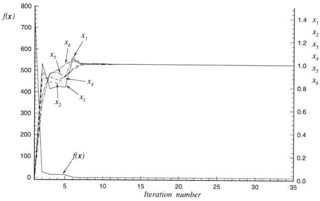
Unconstrained minimization problems are tested first. The number of iterations re-quired for the converged solutions is summarized in Table 2.1. Convergence history of the test problem No. 2-3 is shown in Figure 2-1.

(34)

Problem number Number of variables,n Number of iterations

2-1 2 20

2-2 2 20

2-3 6 35

2-4 10 201

Table 2.1: Performance of the optimization program for unconstrained optimization test problems

Test Problem No. 2-1

Objective function f(x) = 4(zl - 5)2 + (z2 - 6)2

Equality constraints none Inequality constraints none Starting point Xo - (8, 9)T

f(xo)

= 45 Solution from [60] = (5, ₆)T f(b) = 0 Present method x = (5.000, 6.0 00)T f(t) = 0.000

(35)

Test Problem No. 2-2 Objective function u2 + u2 + u2

ui = ci - x1

(1

- xi)

cl = 1.5, c2 = 2.25, c3 = 2.625

X = (x1,x2)T Equality constraints none Inequality constraints none

Starting point xo = (2, 0.2)T

f(xo) = 0.5298

Solution from [60] 5 = (3, 0.5)T

Present method t = (3.000, 0.5 00 0)T

f(t) = 0.000

Objective function f(x) = 10 E =1(16 - i)(xi - 1)2

x = (X1, 2, X 3, X4, X5, X6)T

Equality constraints none

Inequality constraints none

Starting point Xo = (0, 0, 0, 0, 0, O)T

f(xo) = 750

Solution from [60] t = (1, 1, 1, 1, 1, )T

f () = 0

Present method t = (1.000, 1.000, 1.000, 1.000, 1.000, 1.000)T f(.) = 0.000

(36)

f(x) 800 700 600 500 400 300 200 100 0 5 10 15 20 25 30 35 Iteration number

Figure 2-1: Convergence history of the present method for test problem No. 2-3

Objective function f(x) = [1 i3(x,- 1)2]1/3

X - (Xl7, x2 ,X3 4 5,X Z, X6 7 8X9, 10)T Equality constraints none

Starting point

Xo

= (0, 0, 0, 0, 0, 0, 0, 0, O, )T f(xo) = 14.4624 Solution from [60] = (1, 1, 1, 1,1, 1, 1, 1, )T f(t) = 0 Present method _{z = (1.000, 1.000, 1.000, 1.000, 1.000,} 1.000,1.000, 1.000, 1.000, 1.000)T =f(t) = 0.000 1.4 _x, x2 1.2 _x 3 x₄ 1.0 _X x₆ 0.8 0.6 0.4 0.2 0.0

(37)

2.5.2 Constrained Optimization Problem

Several constrained optimization test problems are used to test the performance of the program in this section. Table 2.2 summarizes the test problems used.

Objective function f(x) = 9 - 8x1 - 6x2 - 4x3 + 2x2 + 2x2 + x1 +2xlx 2 + 2x1x3

x = (x1, X2, 3)T

Equality constraints none

Inequality constraints g1 (x) = x1 + x2 + 2x3 - 3 < 0

g

2

(x) = -XZ

<

0 g

3

(x) = -x

2

< 0

g

4

(x)

=

-ZX

3

0

Starting point so = (0.5, 0.5, 0.5)T f (xo) = 2.25 Solution from [26] : = (1.3333, 0.7778, 0.4 4 4 4)T f(t) = 0.1111 Present method t = (1.3333, 0.7778, 0.4 4 4 4)T

f(t)

= 0.1111

(38)

Test Problem No. 2-6

Objective function f(x) = (xI - 1)2 + (x2 - 2)2 + (x3 - 3)2 (x4 - 4)2

x=

(1,

, •,x

)T

Equality constraints hi(x) = x, - 2 = 0

h2

=

x

2

+

X2

- 2 =

0

Starting point Xo = (1, 1,1, 1)T f(xo) = 14 Solution from [26] a = (2, 2, 0.8485, 1.1314)T

f(t)

=

13.8579

Present method x = (2.0000, 2.0000, 0.8485, 1.13 1 4)T f(;) = 13.8579

Objective function f(x) = _, =1 l aij(x? + xi + 1)(x + xj + 1)

S=

(

1

,

X

2

, ..

16 )T

Equality constraints hi(x) = E16 bijz - c = 0

i = 1,...,8

aij, bij, and ci are given in Appendix B Inequality constraints gi(X) = -xi < 0

gi+

16

(x)

= xi

-

5 < 0

i= 1,...,16 Starting point

Xo

= (10, 10, 10, 10, 10, 10, 10, 10, 10, 10, 10, 10, 10, 10, 10, 10)T f(xo) = 566766 Solution from [26] : = (0.03985, 0.7920, 0.2029, 0.8444, 1.1270, 0.9347, 1.6820, 0.1553, 1.5679,0, 0, 0,0.6602, 0,0.6743, 0)T f (t) = 244.8997 Present method : = (0.03985, 0.7920, 0.2029, 0.8444, 1.2699, 0.9347, 1.6820, 0.1553, 1.5679, 0, 0, 0, 0.6602, 0, 0.6742, 0)T f (f:) = 244.8997

(39)

Table 2.2: Constrained optimization test problems

Problem no. No. of variables No. of equality constraints No. of inequality constraints

n 1 m

2-5 3 0 4

2-6 4 2 0

(40)

Chapter 3 Analysis of Cavitating Propellers

by Vortex Lattice Method

The analysis of the flow around a cavitating propeller subject to non-uniform inflow is required at each design optimization iteration. Since this analysis is made a number of times in the course of optimization, it MUST be computationally efficient. For this reason, a vortex lattice method was chosen. A vortex lattice analysis method for cavitating propellers in nonuniform flow developed at MIT is HPUF-3A. A brief description of HPUF-3A is given in this chapter.

3.1 Vortex Lattice Method

The presence of a propeller is represented by the distribution of singularities (vortices and sources) on the blade mean camber surface and its assumed wake surface. The unknown strength of the singularities is determined by applying the kinematic and dynamic boundary conditions at some appropriate control points.

The basic assumptions are :

(41)

* The wake consists of the transition wake, where the roll up and and contraction occur, and the ultimate wake, where the trailing vortices become a concentrated tip vortex. This is illustrated in Figure 3-1.

* There is no roll up in the transition wake.

* Given inflow is an effective wake, which is the difference between the total velocity in the presence of the propeller and the propeller induced velocity. * Sources representing the blade thickness are independent of time and

deter-mined by a spanwise application of thin wing theory.

* The formation and decay of the cavity occurs instantaneously depending only on whether the pressure exceeds the vapor pressure.

* Cavity starts at the leading edge of the blade and vanishes at the cavity trailing edge.

* Cavity thickness is constant across each strip in the spanwise direction and varies linearly along each cavity panel in the chordwise direction.

* There are no spanwise effects in the cavity closure condition.

* Viscous force is computed based on the frictional drag coefficient, Cf, which is applied uniformly on the wetted surface of the blade.

HPUF-3A has been continuously modified since its first version by Lee [47] in

1979. The major modifications include:

1. Nonlinear leading edge correction to the cavity solution [37]. 2. Inclusion of the hub effect via images [38].

3. Supercavitating sections, which have finite trailing edge thickness [45]. 4. Blade geometry representation by B-splines [51].

5. Wake alignment [58]. This is the version that has been used in the present optimization program.

(42)

transition

-E Z

timate wake

= 0.83

x

Figure 3-1: Wake model used in HPUF-SA

transiti

wake

(43)

3.2 Blade Geometry

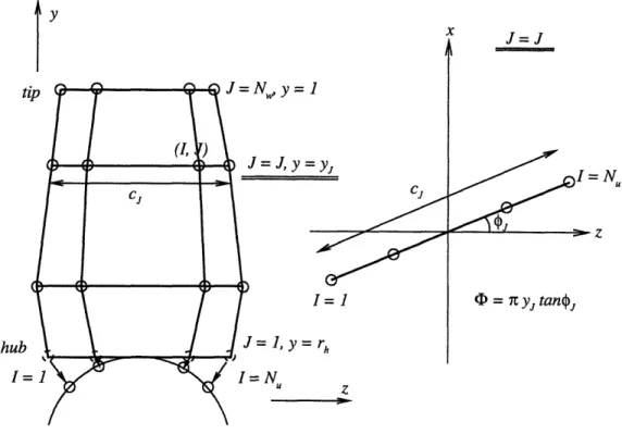
The coordinate systems and the propeller geometrical notation are shown in Figure 3-2. A propeller-fixed cartesian coordinate system is first defined with the x axis positive downstream. The y axis is normal to x axis at any angular orientation relative to the key blade. The z axis completes the right hand system. A cylindrical coordinate system is defined in the usual way.

X • X

r=

y+

2 _(3.1)

0 =

tan-The radial distributions of skew, 0m(r), and rake, xm(r), define the mid-chord line of the blade as illustrated in Figure 3-3. The leading and trailing edges of the blade are constructed by passing a helix of pitch angle O(r) through the mid-chord line.

xI,t(r) = xm(r):F sin O(r) 2

c(r)

01,t(r) = Om(r) : 2 cosO (r) (3.2)

yi,t(r) = r cos 6,t(r)

zi,t(r) = rsine ,t(r)

where c(r) is the chord length at the radius r , and the subscripts 1 and t denote the leading and trailing edges, respectively.

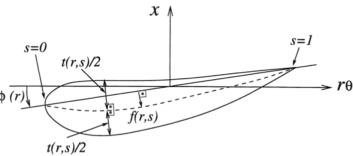
The camber f(r, s) is measured on the cylindrical surface of radius r normal to the nose-tail helix, where s is a non-dimensional chordwise coordinate, which is 0 at the leading edge and 1 at the trailing edge.

Finally, the thickness t(r, s) is added symmetrically to the camber line on the cylinder in the normal direction to the mean camber surface. This is shown in Figure

(44)

z

Figure 3-2: Coordinate systems and geometrical notations in HPUF-3A, adapted from [25]

(45)

z

:ylin

is

r

nean

X

Figure 3-3: Radial distribution of skew and rake, adapted from [35]

(46)

X

s-O

t(r,

N-1A

4 t(r,

s)/2

Figure 3-4: Construction of blade section from mean camber line and thickness form

3-4. =

m(r)

+

c(r)

(

-= _{Om(r) + c(r)} s8-=

r cos O(r, s)

= r sin , (r, s) 1)

21

2 sin

q(r)

-

f(r, s) cos

q(r)

cos (r)+

r

sin O(r)

f(r, S)

_T

The maximum values of f(r, s) and t(r, s) at radius r are denoted as the maximum camber,

fo(r),

and the maximum thickness, to(r), respectively.

3.3 B-spline Representation of the Blade

The B-spline representation of the blade is attractive in several ways and has been included in HPUF-3A.

In the traditional geometry definition described in section 3.2, tabular data for

s=1

7-ro

xC(r, S) 6,(r, S) yc(r, S)

(3.3)

(47)

radial distributions of pitch, rake, and skew, and chordwise distributions of camber and thickness are usually given. Inaccuracy arises due to the interpolation process necessary to determine the actual blade surface. By using B-splines, all points on the surface are defined uniquely. Another advantage of B-splines is that the blade may be defined with a relatively few number of parameters. This is particularly convenient for designing blades by numerical optimization. The number of parameters, also of the design variables, reflects the computational effort of the optimization method.

3.3.1 Cubic B-spline Curves and Surfaces

In HPUF-3A, cubic B-splines, which is a subset of Non- Uniform Rational B-Splines

(NURBS), are used. To see some properties of B-splines, B-spline curves are reviewed

first following Patrikalakis [55].

Non-uniform B-spline curves are defined as :

N,-1

P(u) = [Z(u), y(u), z(u)]= E diNi,k(u) (3.4)

i=O

N

> k

where,

di : B-spline control points

Ni,k (u) : B-spline basis of order k (piecewise polynomial of degree k - 1)

u : parameter in the interval to < u < tNu+k-1

T =

It,,

= tj =

...

= tk- <

k <_

tk+<

<

tNu_1 < tNu =-..= tNu+k-11

k equal values Nu-k internal knots k equal values

knot vector, which has total N, + k knots

B-spline basis Ni,k (u) is determined from the following required properties. 1. Partition of unity

Nu-1

E

Ni,k (u) = 1 (3.5)

(48)

2. Positivity

Ni,k(u) > 0

3. Local support (change of one vertex, di affects curve locally)

Ni,k(u) = 0

if u ý [ti, ti+k]

4. Ck- 2 continuity

Ni,k (U) is (k - 2) times continuously differentiable at simple knots. If a knot has a multiplicity equal to p (< k),

tj = tj+1 =... - tj+p-1

and Ni,k (u) is (k - p - 1) times continuously differentiable.

Ni,k (u) may be obtained recursively as, for example, in Yamaguchi [74].

Ni,i(u) =

0 u - ti Ni,k(u) = i -N ti+k-1 - ti U E [ti, ti+l) ti+k - u ,k-1) + tk - U Ni+,k-1 (u) ti+k - ti+1l

If a "0/0" situation occurs, that term is set equal to 0 in equation (3.9).

Since in most propeller applications, continuity in curvature but not in higher order derivatives is desirable, k = 4 (cubic B-splines) is chosen. Figure 3-5 shows the cubic

B-spline basis (k = 4) for N, = 7.

Figure 3-6 illustrates control points and the corresponding cubic B-spline curve.

Cubic B-spline surfaces are defined similarly as follows. Nu-1

P(u, w) = [x(u, w), y(u, w), z(u, w)] =

i=O N,- 1

E

dijNi,4(u)Nj,4j(w) j=0 (3.10) where

dij : B-spline control points

(3.6)

(3.7)

(3.8)

Design of cavitating propeller blades in non-uniform flow by numerical optimization