HAL Id: hal-00534653
https://hal.archives-ouvertes.fr/hal-00534653
Submitted on 10 Nov 2010HAL is a multi-disciplinary open access archive for the deposit and dissemination of sci-entific research documents, whether they are pub-lished or not. The documents may come from teaching and research institutions in France or abroad, or from public or private research centers.
L’archive ouverte pluridisciplinaire HAL, est destinée au dépôt et à la diffusion de documents scientifiques de niveau recherche, publiés ou non, émanant des établissements d’enseignement et de recherche français ou étrangers, des laboratoires publics ou privés.
Multi-emitter and multi-receiver probe for long cortical
bone assessment
Jean-Gabriel Minonzio, Maryline Talmant, Pascal Laugier
To cite this version:
Jean-Gabriel Minonzio, Maryline Talmant, Pascal Laugier. Multi-emitter and multi-receiver probe for long cortical bone assessment. 10ème Congrès Français d’Acoustique, Apr 2010, Lyon, France. �hal-00534653�
10ème Congrès Français d'Acoustique
Lyon, 12-16 Avril 2010
Multi-emitter and multi-receiver probe for long cortical bone assessment
Jean-Gabriel Minonzio, Maryline Talmant, Pascal Laugier Laboratoire d'Imagerie Paramétrique, 15 Rue De L'école De Médecine 75006 Paris
UPMC Univ Paris 06, CNRS UMR 7623 [email protected]
Different quantitative ultrasound techniques are currently developed for clinical assessment of human bone status. This paper is dedicated to axial transmission: emitters and receivers are linearly arranged on the same side of the skeletal site, preferentially the forearm, a referenced site to predict fracture risk in case of osteoporosis. In several clinical studies, the signal velocity of the earliest temporal event has been shown to discriminate osteoporotic patients from healthy subjects. However, a multi parameter approach might be relevant to improve bone diagnosis and this be could achieved by accurate measurement of guided waves phase velocities. Clinical requirements and bone/soft tissue heterogeneities constrain the length probe to about 10 mm. Thus efficiency of conventional spatial-temporal Fourier transform is reduced. Efficiency of time-frequency techniques was shown to be moderate in other studies. Signal processing to obtain reliable guided wave velocities is a key point. A technique, taking benefit of using both multiple emitters and multiple receivers, is proposed. The guided mode phase velocities are obtained using a projection in the singular vectors basis. Those are determined by the singular values decomposition of the response matrix between the two arrays at fixed frequencies. This method was first validated on metallic plates, enabling us to recover accurately guided waves phase velocities for moderately large array.
1 Introduction
Elastic waves are widely used in material characterization. For example, guided waves, such as Lamb waves, are used to characterize plate or tube [1]. Structural and material properties can be characterized by fitting measured to theoretical guided waves phase velocities. The two dimensional spatial–temporal Fourier transform is one of the usual methods used to determine the guided mode phase velocities [2]. Nevertheless this approach requires a large distance probed by the receivers. Practical constraints, as in clinical inspection of cortical bones, reduce the inspected spatial length and therefore the efficiency of this technique. That is why an original approach is presented in this paper to enhance the two-dimensional Fourier transform approach, using the Singular Values Decomposition (or SVD) applied to the configuration of a multi-emitter and multi-receiver array in contact with the object to be characterized. SVD is a widely used filtering tool [3]. The aim of this paper is to introduce an original method of measurement of the guided mode phase velocities in the context of ultrasonic cortical bone testing in the axial transmission geometry [4].
2 Theory
2.1 Response matrix
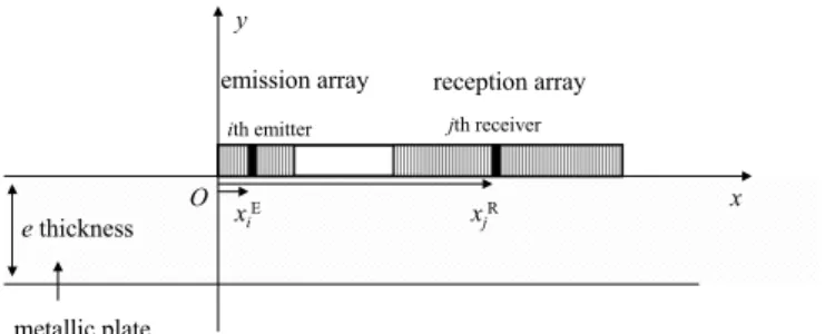
Two arrays are used in contact with a metallic plate, using coupling gel (Fig. 1). Superscripts E and R refer respectively to the emission and reception arrays. Thus the emission array contains NE emitters of position x
iE, with 1≤
i ≤ NE. Likewise, the reception array contains NR receivers
of position xjR, with 1≤ j ≤ NR. Define the NR×1 vector R
containing the NR Fourier transforms R
j(f) of rj(t), with f the
temporal frequency. Likewise, the NE×1 vector E contains
the NE Fourier transforms E
i(f). The relation between the
two vectors R and E writes, at a given frequency
R = H. E , (1)
with H the NR×NE matrix containing the elements H
ji(f)
equal to the Fourier transform of the impulse responses
hji(t). The R matrix, called afterward “response matrix”, is
characteristic of the “emission – scattering medium – reception” system.
x
ith emitter jth receiver
metallic plate e thickness
y
xiE xjR
emission array reception array
O
Figure 1: Geometry of the problem: the emission and reception arrays are in contact with the metallic plate.
2.2 Singular vectors basis
The Singular Value Decomposition (SVD) of the response matrix R writes
E * 1 N t n n n n σ = =
∑
R U V , (2)where the notations t and * denote the transpose and
conjugation operations. The number of experimental singular values σn is equal to minimum size of the arrays,
i.e. the minimum between NE and NR, equal in the following
to NE. The notation V
n refers to an emission singular vector,
of dimension NE×1, and U
n to a reception singular vector, of
dimension NR×1. These two vectors are associated with the
singular value σn.
The singular vectors Un (resp. Vn) are normalized and
define an orthogonal basis of the received (resp. emitted) signals. In particular any spatial plane wave can be expressed in the reception basis. Consider a spatial plane wave epw(k) with k = 2πf/c and c the phase velocity c,
defined on the jth receiver as
( )
R R 1 exp i pw j j e kx N = , (3)The previous vector is defined normalized. The expression on the basis defined by the reception singular vectors Un is E 1 N pw pw n n n= =
∑
e e U U , (4)with the notation < epw | U
n > corresponding to the
Hermitian scalar product, equal to t[epw]* .U
n .
2.3 Noise and signal separation
One of the advantages of the SVD approach is its ability to separate noise and signal subspaces [9]. Indeed, using an intermediate order m corresponding to the limit between the two subspaces, equation (4) can be rewritten with a truncated sum, with n ≤ m. The order m is defined at each frequency using a threshold t1 applied to the singular
values σn. In the following, the signal singular vectors are
retained (for σn ≥ t1) whereas the noise singular vectors (for
σn < t1) are eliminated. Thus the norm of the spatial plane
wave on the basis of the signal subspace becomes
{ } 2 1 n m m pw pw n n ≤ =
∑
= U e e U , (5)with the notation | | used for the modulus of complex
numbers. The value of the threshold t1 is heuristically
chosen, based on an estimation of the signal to noise ratio and on a trade-off between the estimated number of guided modes and the noise level. That threshold may also vary with frequency. Examples are shown in Sec. 3 and Fig. 2.
2.4 Evaluation of the guided mode phase velocities
The norm of the spatial plane wave expressed on the signal (or retained) singular vectors in (5) is used to form an image in the (k, f) plane. To enhance the contrast between the low and high values, the square of the norm is used in the following. As m, the dimension of the signal subspace, is less than the number of receivers NR, i.e. the dimension of
the vector epw, the basis defined by the signal reception
singular vectors Un≤m is incomplete. It implies that the norm
defined by (5) is less than 1. Consequently, each pixel (k, f) of the image ranges from 0 to 1.
The value of the pixel reflects how the spatial plane wave is represented in the basis of the signal subspace. On the one hand, if the value is small compared to 1, the spatial plane wave is absent of the received signals. On the other hand, if the value is close to 1, the spatial plane wave corresponds to a guided wave, present in the received
signals. A second threshold t2 is then applied to the image in
order to reduce the range from t2 to 1. Thus a function Norm
is defined in the (k, f) plane as
(
)
{ } { }(
)
{ } 2 2 2 2 2 , , 0 n m n m n m pw pw pw Norm k f if t Norm k f if t ≤ ≤ ≤ ⎧ = ≥ ⎪ ⎨ ⎪ = < ⎩ U U U e e e , (6)The maxima of the function Norm(k, f) provide the phase velocities of the guided mode present in the signal subspace. In the examples shown in Sec. 3, the value of that second threshold t2 is heuristically chosen equal to 0.4 as
shown in Fig. 4.
3 Experimental results and discussion
3.1 Experimental set up
The probe developed at the LIP (Laboratoire d’Imagerie Paramétrique), for the bone characterization, consists of NE
of emitters is equal to 5 and the number of receivers NR is
equal to 32. Thus the number of emitters, which is less than the number of receivers, corresponds to the number of experimental singular values. A coupling gel is used in order to improve the acoustical impedance matching. Emitted signals are pulses with bandwidth about 0.5−2 MHz. The reception array pitch is equal to 0.80 mm. The experimental scattering medium is a 2 mm thickness copper plate. The free plate guided modes are given by the Rayleigh-Lamb dispersion equation [1]. No attenuation is considered in this model. The modes are labelled considering their symmetry or anti-symmetry and their cut-off frequencies, i.e. Sn and An [1].
3.2 Resolution and evaluation domain of the system
The resolution can be estimated considering the size of the main lobe of the sinc function, given by the scalar
product between a reception singular vector Un
corresponding to a guided mode kn and a spatial plane wave
epw(k) [Eq. (3)]. With LR the size of the reception array, the
resolution condition writes R 2 k L π Δ ≥ . (7)
Furthermore, the Shannon criterion is verified when k is less than π/p, with p the array pitch. Thus the range 2π/LR ≤
k ≤ π/p corresponds to the evaluation domain, where the
guided mode phase velocities k can be evaluated.
3.3 Experimental results, comparison with the 2D Fourier transform
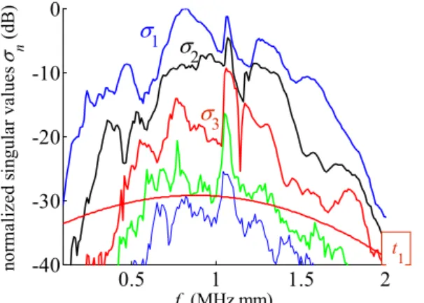
Figure 2 shows the experimental singular values σn as
function of the frequency f. The number of experimental singular values, i.e. 5, corresponds to the number of emitters. At low frequency, only the two first singular values are significant, whereas for f > 1 MHz, the number of significant singular values ranges from 3 to 5. It corresponds to the number m of significant singular vectors used in (6). It depends on the signal to noise threshold t1,
shown with a curved line, heuristically fixed around −30dB. The different peaks correspond to thickness resonance of
guided modes. For example, the thin peak for f = 1.1 MHz corresponds to the ZGV resonance [2].
0.5 1 1.5 2 -40 -30 -20 -10 0 f (MHz.mm) no rm alized s in gu lar v alu es σ (dB) n σ3 σ2 σ1 t1
Figure 2: Singular values versus frequency (MHz) for a 2 mm thick copper plate. The signal to noise threshold t1 is
shown with a curved dashed line.
Figure 3(a) shows the image Norm(k, f) defined by Eq. (6) using the signal singular vectors, i.e. the singular vectors associated with singular values bigger than the threshold t1 shown in Fig. 2. As expected, the value of the
pixels ranges from 10-8 to 0.96. The guided mode phase
velocities are shown as trajectories in the (k, f) plane. The width of each trajectory corresponds to the resolution given by Eq. (7). Figure 3(b) shows the two-dimensional spatial-temporal Fourier transform for comparison. Each line (or frequency) is normalized by its maximum.
k (rad.mm-1) f (M H z) Norm(k, f) -1 0 1 2 3 0.5 1 1.5 2 0 0.2 0.4 0.6 0.8 1 A1 A0 S0 t2 S1 S2 (a) k (rad.mm-1) f (M H z) 2D Fourier transform -1 0 1 2 3 0.5 1 1.5 2 0 0.2 0.4 0.6 0.8 1 (b) Figure 3: Norm(k, f) (a) and 2D Fourier Transform (b) for a 2 mm thick copper plate. The maxima of the Norm function are more clearly defined.
The results given by the two methods are globally similar. However, the Norm function allow a better ability to evaluate phase velocities as illustrated in Fig. 4 for a fixed frequency shown as dashed line in Fig. 3(a). The maxima of the Norm function ranging from 0.4 to 0.9 are clearly defined, contrary to the maxima of the two dimensional Fourier transform. It shows that this original technique can be applied to noisy medium such as cortical bone. -1 0 1 2 3 4 0 0.1 0.2 0.3 0.4 0.5 0.6 0.7 0.8 0.9 1 f = 1.13 MHz k (rad.mm-1) No rm ( k, f ) 2DFT Norm(k, f ) S2 S 2 S0 A0 A1 t2
Figure 4: Comparison of the two methods: Norm(k, f) and 2D Fourier transform, for f = 1.13 MHz. This frequency shown as a dashed line in figure 3(a). The ability to extract phase velocity is improved using the Norm function. The second threshold t2 is shown with a horizontal dashed line.
Conclusion
An original method for evaluating the guided mode phase velocities using arrays in contact (an emission array and a reception array) is exposed in this paper. The ability to estimate the guided mode phase velocities is improved compared to the results obtained with the spatial-temporal Fourier transform. Further applications will concern in particular the evaluation of elastic properties of cortical bone with a reduced inspected spatial length due to practical constraints. These results open a perspective towards a good evaluation of the thickness and/or the transverse and longitudinal bulk waves velocities. Attenuation and non-isotropic medium will be taken into account.
Acknowlegment
This work has been funded by the ANR TecSan under EVA project.
References
[1] D. Royer, and E. Dieulesaint, “Elastics waves in
solids 1 : Free and guided propagation,” Springer, Berlin, p. 317 (1999).
[2] C. Prada, D. Clorennec, and D. Royer, “Local
vibration of an elastic plate and zero-group velocity
Lamb modes,” J. Acoust. Soc. Am. 124, 203−212
(2008).
[3] T. G. Kolda and B. W. Bader, “Tensor
Decompositions and Applications,” SIAM Review
51, 455−500 (2009).
[4] E. Bossy, M. Talmant, M. Defontaine, F. Patat, and
P. Laugier, “Bidirectional axial transmission can improve accuracy and precision of ultrasonic velocity measurement in cortical bone: a validation on test materials,” IEEE Trans. Ultrason. Ferroelectr. Freq. Control. 51, 71−79 (2004).
[5] P. Moilanen, P. H. F. Nicholson, V. Kilappa, S.
Cheng, and J. Timonen, “Measuring guided waves in long bones: Modeling and experiments in free and immersed plates,” Ultrasound in Medecine and Biology 32, 709−719 (2006).
[6] V. C. Protopappas, I. C. Kourtis, L. C. Kourtis, K. N.
Malizos, C. V. Massalas, and D. I. Fotiadis, “Three-dimensional finite element modeling of guided ultrasound wave propagation in intact and healing
long bones,” J. Acoust. Soc. Am. 121, 3907−3921
(2007).
[7] D. Ta, W. Wang, Y. Wang, L. H. Le, and Y. Zhou,
“Measurement of the dispersion and attenuation of cylindrical ultrasonic guided waves in long bone,” Ultrasound in Medecine and Biology 35, 641−652 (2009).
[8] M. Sasso, M. Talmant, G. Haiat, S. Naili, and P.
Laugier, “Analysis of the most energetic late arrival in axially transmitted signals in cortical bone,” IEEE Trans. Ultrason. Ferroelectr. Freq. Control, 56, 363−2470 (2009).
[9] M. Davy, J. G. Minonzio, J. de Rosny, C. Prada, and
M. Fink, “Influence of noise on subwavelength imaging of two close scatterers using time reversal method: Theory and Experiments,” Progress in Electromagnetic Research 98, 333−358 (2009).