HAL Id: tel-01362134
https://tel.archives-ouvertes.fr/tel-01362134
Submitted on 8 Sep 2016HAL is a multi-disciplinary open access archive for the deposit and dissemination of sci-entific research documents, whether they are pub-lished or not. The documents may come from teaching and research institutions in France or abroad, or from public or private research centers.
L’archive ouverte pluridisciplinaire HAL, est destinée au dépôt et à la diffusion de documents scientifiques de niveau recherche, publiés ou non, émanant des établissements d’enseignement et de recherche français ou étrangers, des laboratoires publics ou privés.
Information Theory Oriented Image Restoration
Cesario Vincenzo Angelino
To cite this version:
Cesario Vincenzo Angelino. Information Theory Oriented Image Restoration. Signal and Image processing. Université Nice Sophia Antipolis, 2011. English. �tel-01362134�
´E
COLE
D
OCTORALE
STIC
Science et Technologies de l’Information et de la Communication
TH `ESE
pour obtenir le titre de
Docteur en Sciences
de l’Universit´e de Nice - Sophia AntipolisMention : Automatique, Traitement du Signal et des Images pr´esent´e et soutenue par
Cesario Vincenzo A
NGELINOLaboratoire I3S (Informatique, Signaux et Syst`emes de Sophia Antipolis)
I
NFORMATION
T
HEORY
O
RIENTED
I
MAGE
R
ESTORATION
Th`ese dirig´ee par Michel BARLAUD et Eric DEBREUVE Soutenue publiquement le 9 septembre 2011 devant le jury compos´e de
Luigi PAURA Professeur des Universit´es (Federico II Naples) Rapporteur
Philippe SALEMBIER Professeur des Universit´es (Barcelona) Rapporteur
Michel BARLAUD Professeur des Universit´es (Nice-Sophia Antipolis) Directeur de th`ese
Eric DEBREUVE Charg´e de recherche CNRS Directeur de th`ese
UNIVERSITA DEGLI` STUDI DI NAPOLI“FEDERICO II”
DIPARTIMENTO DI INGEGNERIAELETTRONICA
E DELLE TELECOMUNICAZIONI
DOTTORATO DI RICERCA IN
INGEGNERIAELETTRONICA E DELLE TELECOMUNICAZIONI
I
NFORMATION
T
HEORY ORIENTED
I
MAGE
R
ESTORATION
C
ESARIOV
INCENZOA
NGELINOIl Coordinatore del Corso di Dottorato I Tutori
Ch.mo Prof. Niccol´o RINALDI Ch.mo Prof. Michel BARLAUD
travers de la minimisation d’une ´energie. Ces ´energies appartiennent `a la classe non param´etrique au sens o`u elles ne font aucune hypoth`ese param´etrique sur la distribution des donn´ees. Les ´energies sont exprim´ees directement en fonction des donn´ees consid´er´ees comme des variables al´eatoires. Toutefois, l’estimation non param´etrique classique repose sur des noyaux de taille fixe moins fiables lorsqu’il s’agit de donn´ees de grande dimension. En particulier, des m´ethodes r´ecentes dans le traitement de l’image d´ependent des donn´ees de type ”patch” correspondant `a des vecteurs de description de mod`eles locaux des images naturelles, par exemple, les voisinages de pixels. Le cadre des k-plus proches voisins r´esout ces difficult´es en s’adaptant localement `a la distribution des donn´ees dans ces espaces de grande dimension. Sur la base de ces pr´emisses, nous d´eveloppons de nouveaux algorithmes qui s’attaquent principalement `a deux probl`emes du traitement de l’image : la d´econvolution et le d´ebruitage. Le probl`eme de la restauration est d´evelopp´e dans les hypoth`eses d’un bruit blanc gaussien additif puis successivement adapt´es `a domaines tels que la photographie num´erique et le d´ebruitage d’image radar (SAR). Le sch´ema du d´ebruitage est ´egalement modifi´e pour d´efinir un algorithme d’inpainting.
Mots clefs : restauration d’image, th´eorie de l’information, estimation non param´etrique, entropie, mean-shift, d´econvolution, patch, d´ebruitage non local, SAR, despeckling, inpainting d’image.
Abstract: This thesis addresses informational formulation of image processing problems. This formulation expresses the solution through a minimization of an information-based energy. These energies belong to the nonparametric class in that they do not make any parametric assumption on the underlying data distribution. Energies are expressed directly as a function of the data considered as random variables. However, classical nonparametric estimation relies on fixed-size kernels which becomes less reliable when dealing with high dimensional data. Actually, recent trends in image processing rely on patch-based approaches which deal with vectors describing local patterns of natural images, e. g., local pixel neighbor-hoods. The k-Nearest Neighbors framework solves these difficulties by locally adapting the data distribution in such high dimensional spaces. Based on these premises, we develop new algorithms tackling mainly two problems of image processing: deconvolution and denoising. The problem of denoising is developed in the additive white Gaussian noise (AWGN) hypothesis and successively adapted to no AWGN realm such as digital photography and SAR despeckling. The denoising scheme is also modified to propose an inpainting algorithm.
Keywords: image restoration, information theory, nonparametric estimation, en-tropy, mean-shift, deconvolution, patch, nonlocal denoising, SAR, despeckling, im-age inpainting.
Contents
Acknowledgments vi List of Figures xi List of Tables xv 1 Introduction 1 1.1 Context . . . 11.2 Contributions of the thesis . . . 2
2 ESTIMATION OF SOME STATISTICAL MEASURES 5 2.1 Introduction . . . 5
2.2 Kernel density estimation (KDE) . . . 6
2.2.1 Multivariate KDE. . . 6
2.2.2 Bandwidth selection . . . 7
2.3 Nonparametric entropy estimation . . . 10
2.3.1 Plug-in estimates . . . 10
2.3.2 The kNN framework . . . 10
2.4 Entropy derivative and Mean Shift . . . 11
2.5 Mean-Shift approximation . . . 13
2.5.1 Based on fixed kernel size . . . 13
2.5.2 Based on variable kernel size. . . 13
2.6 Conclusion . . . 14
I Deconvolution 19 3 ENTROPY-BASED DECONVOLUTION 21 3.1 Introduction . . . 21
3.2 State of the art . . . 22
3.2.1 Deterministic approach . . . 22
3.2.2 Statistical methods . . . 23
3.2.3 Why using entropy? . . . 24
3.3 Proposed method: MRED. . . 24 vii
3.3.1 Minimizing the residual entropy . . . 24
3.3.2 Energy lower bound . . . 25
3.3.3 Energy derivative . . . 26
3.4 Experimental Results . . . 27
3.5 Discussion and perspectives . . . 29
II Denoising 37 4 PATCH-BASED DENOISING 39 4.1 Introduction . . . 39
4.2 Neighborhood Denoising: state of the art. . . 40
4.2.1 The UINTA algorithm . . . 40
4.2.2 Non-Local Means. . . 40
4.2.3 Block Matching 3D (BM3D) . . . 41
4.3 Proposed method: PCkNN . . . 43
4.3.1 Entropy-based formulation . . . 43
4.3.2 Energy lower bound . . . 43
4.3.3 Energy derivative . . . 45
4.3.4 Full patch denoising . . . 47
4.3.5 Confidence-based patch combination . . . 48
4.3.6 Summary of the algorithm . . . 49
4.4 Experiments . . . 49
4.5 Improving PCkNN with robust patch similarity . . . 55
4.5.1 Robustness to noise. . . 59
4.5.2 Transformation invariance . . . 59
4.5.3 Effect of the transformations: A toy example . . . 59
4.6 Conclusion and perspectives . . . 60
III Specific applications 63 5 DIGITAL PHOTOGRAPHY 65 5.1 Introduction . . . 65
5.2 Noise and sensor . . . 65
5.2.1 Sensor and image acquisition. . . 65
5.2.2 Noise model . . . 67
5.2.3 Parameters estimation . . . 69
5.2.4 Demosaicing . . . 70
5.3 Adapting PCkNN to CFA images . . . 70
5.3.1 Intra-channel denoising. . . 71
CONTENTS ix
6 SAR despeckling 81
6.1 Introduction . . . 81
6.2 State of the art . . . 81
6.2.1 Spatial domain techniques . . . 81
6.2.2 Wavelet based techniques . . . 82
6.2.3 Non-local techniques . . . 83
6.3 The BM3D algorithm and its SAR-oriented version . . . 84
6.4 Proposed SAR-oriented modifications in detail . . . 85
6.4.1 Block similarity measure . . . 85
6.4.2 Group shrinkage . . . 87
6.4.3 Aggregation. . . 89
6.5 Experimental results . . . 90
6.5.1 Gold standards and parameter setting . . . 90
6.5.2 Results with simulated speckle . . . 91
6.5.3 Results with actual SAR images . . . 94
6.6 Conclusion and future work. . . 97
7 Digital Image Inpainting 103 7.1 Introduction . . . 103
7.2 State of the art . . . 106
7.2.1 PDE based algorithms . . . 107
7.2.2 Exemplar-based texture synthesis . . . 108
7.3 Proposed algorithm and results . . . 109
7.4 Conclusion and perspectives . . . 110
Conclusion 115 IV Appendix 117 A Derivative of the residual entropy E 119 A.1 Definitions and notations . . . 119
A.2 Derivative of p . . . 120
A.3 Derivative of E . . . 121
B Computation of the second order term χ(w) of the entropy derivation125 B.1 Gaussian Residual PDF . . . 125 B.1.1 Gaussian Kernel . . . 125 B.1.2 Epanechnikov Kernel . . . 126 B.2 Histogram Residual pdf . . . 126 B.2.1 Gaussian Kernel . . . 127 B.2.2 Epanechnikov Kernel . . . 128
List of Figures
2.1 Kernel density estimation performance on a 1-D Gaussian mix-tures for different bandwidth. Actual distribution is in black, ker-nel density estimate is in blue and kerker-nels are in red. h is the plugin estimate using rule of thumb, from left to right, top to bottom: ac-tual PDF, PDF estimated with 0.2h, PDF estimated with h, PDF estimated with 5h.. . . 8
2.2 Multivariate kernel density estimation performance on a 2-D Gasian mixtures for different bandwidth. h is the plugin estimate us-ing rule of thumb, from left to right, top to bottom: actual PDF, PDF estimated with 0.2h, PDF estimated with h, PDF estimated with 5h. . . 9
2.3 Entropy estimation of different PDF with relative errors. Circles represent Parzen, i.e. fixed bandwidth, estimation. Squares repre-sent kNN estimator (k = 10) and triangles reprerepre-sent the estimator presented in [NK07]. . . 16
2.4 3D data uniformely distributed on embedded 2D manifolds. In lexicographic order: Plane, Spherical surface, Circle (intersection between the Plane and a sphere), Ring torus and Swiss roll. Esti-mated entropies are given in Table 2.6. . . 17
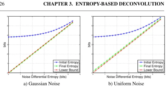
3.1 Residual Entropy as function of noise entropy.Initial residual en-tropy (blue), Final residual enen-tropy (green), Theoretical lower bound (red). . . 26
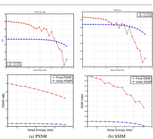
3.2 Algorithm performances for gaussian noise (top) and uniform noise (bottom) as function of noise entropy. (a) Initial (blue) and Final (red) PSNR; (b) Initial (blue) and Final (red) SSIM. . . 29
3.3 Left: Degraded image with a gaussian filter (σ2 = 3), and zero
mean Uniform noise of entropy 2 bits. Right: Residual entropy as function of iterations. . . 31
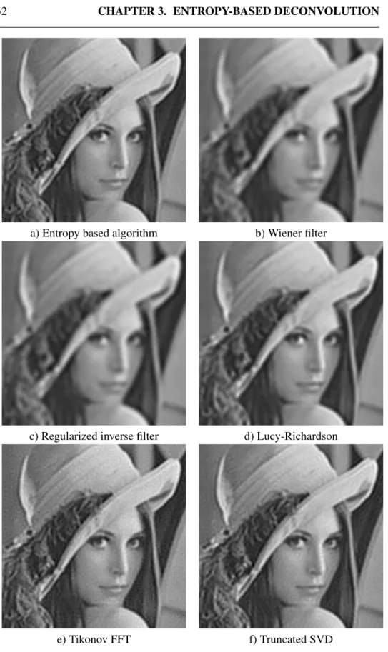
3.4 Deconvoluted images comparison, Uniform noise, entropy 2 bit. . 32
3.5 Deconvoluted images comparison, Gaussian mixture noise, en-tropy 1.85 bits . . . 33
3.6 Mixture noise. Left: Gaussian mixture pdf (entropy 1.85 bits). Right: Gaussian/Uniform mixture pdf (entropy 0.7 bits). . . 34
3.7 Deconvoluted images comparison, Gaussian + Uniform mixture
noise, entropy 0.7 bits. . . 35
4.1 Flowchart of BM3D algorithm [DFKE07b]. . . 42
4.2 Image patch illustration. . . 44
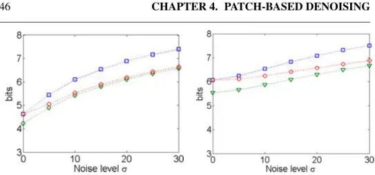
4.3 Behavior of the conditional entropy before and after denoising. Squares represent the conditional entropy, h( ˜X| ˜Y ), of the noisy image. Diamonds represent the conditional entropy, h( ˆX| ˜Y ), after denoising with proposed method. Circles denote the lower bound h(X| ˜Y ). Left: Lena. Right: Mandrill. . . 46
4.4 Patch overlapping illustration. . . 48
4.5 Patch combination step illustration.. . . 50
4.6 Block diagram for PCkNN algorithm. . . 50
4.7 Pseudo code for the proposed PCkNN algorithm. . . 51
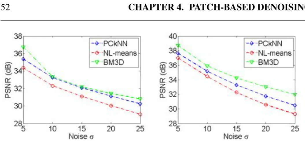
4.8 PSNR for the image Elaine (left) and Lena (right).. . . 52
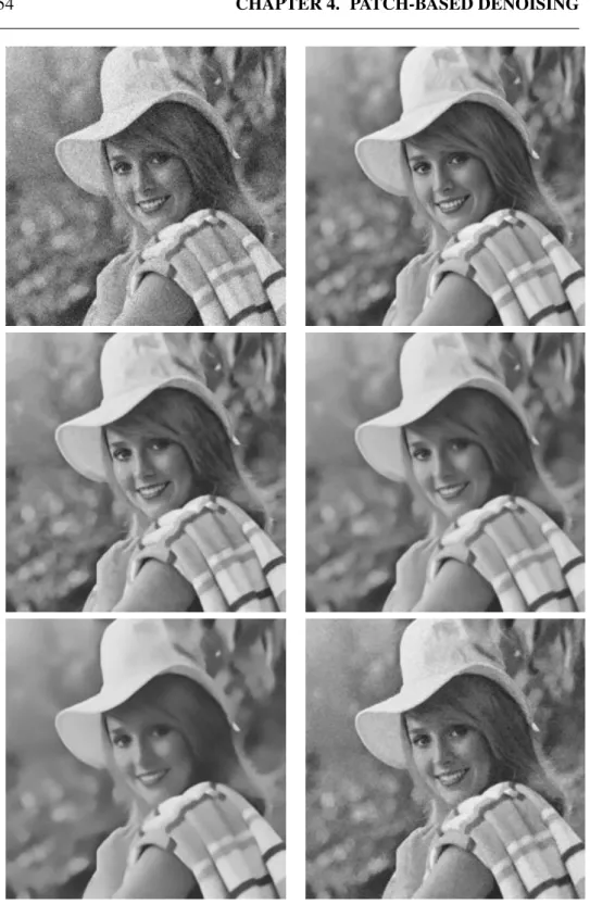
4.9 In lexicographic order: Noisy, Original, BM3D, PCkNN, NL-means, and UINTA.The image Elaine was corrupted with an ad-ditive white Gaussian noise with standard deviation of σ = 25. . . 54
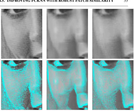
4.10 A close-up on the image Elaine. From left to right: Original, BM3D, and PCkNN. First row: image alone; second row: isolevel lines superimposed on the image.. . . 55
4.11 A close-up on the image Lena. From left to right: Original, BM3D, and PCkNN. First row: image alone; second row: isolevel lines superimposed on the image. . . 56
4.12 A close-up on the image Barbara. From left to right: Original, BM3D, and PCkNN. First row: image alone; second row: isolevel lines superimposed on the image.. . . 57
4.13 Normalized Total Variation. Left: Elaine. Right: Lena. . . 57
4.14 FT Amplitude of the error between the blurred original and the de-noised image. Left BM3D, right PCkNN. First row: Elaine, second row: Lena. . . 58
4.15 Enery Spectrum Density (ESD) (dB) of the reconstruction error. Left: Elaine. Right: Lena.. . . 58
4.16 Effect of the transformations: A toy example. In lexicographic or-der: Original, Noisy, Denoised with no transformations, Denoised with transformations. . . 60
4.17 PSNR plot for the image Elaine. . . 61
4.18 A close-up on the image Elaine of Figure 4.9. From left to right: Original, BM3D, PCkNN and PDC-RS. Top: image alone; bottom: isolevel lines superimposed on the image. . . 61
5.1 Physical properties of Silicon. The images above come from [Nak05]. . . 66
LIST OF FIGURES xiii
5.2 �Foveon. Two different image sensor. Left Conventional CFAc sensor.Right The layered Foveon X3�R sensor. . . . . 67
5.3 Optical system. . . 67
5.4 Properties of noise components. The pictures above are taken from [HK94]. . . 69
5.5 Linear noise model. . . 70
5.6 PSD of the green channel (left) and a red/blue channel (right) from the demosaiced white noise patch using bilinear demosaic-ing [AGPP09]. . . 71
5.7 Intra-channel denoising scheme. Each color channel of the RAW image is denoised separately. The two Green of the Bayer grid are tread separately as well. . . 72
5.8 Professional benchmark image (Courtesy of DxO Labs) used for test. 73
5.9 Professional benchmark image (Courtesy of DxO Labs). RAW im-age (left) and denoised imim-age (right).. . . 74
5.10 Professional benchmark image (Courtesy of DxO Labs). RAW im-age (left) and denoised imim-age (right).. . . 74
5.11 Professional benchmark image (Courtesy of DxO Labs). RAW im-age (left) and denoised imim-age (right).. . . 75
5.12 Professional benchmark image (Courtesy of DxO Labs). RAW im-age (left) and denoised imim-age (right).. . . 75
5.13 Comparison between RAW demosaiced imgages with no denoising (left) and with denoising (right). Particular of the image in Fig. 5.8. (Courtesy of DxO Labs). . . 76
5.14 Inter-channel denoising. The block matching step is modified in order to catch only coherent patches within the search window. . . 77
5.15 Comparison between intra-channel (left) and coherent (right) block matching. . . 77
5.16 Comparison between intra-channel block-matching (left) and co-herent block-matching (right). Particular of the eyes. (Courtesy of DxO Labs). . . 78
6.1 Original images used in the experiments.. . . 92
6.2 Zoom of filtered images with the various techniques for Lena cor-rupted by one-look speckle.. . . 93
6.3 Zoom of filtered images with the various techniques for Napoli corrupted by one-look speckle. . . 94
6.4 Filtered images with the various techniques for target. . . 96
6.5 False alarms (FA) images with the various techniques for target. . 97
6.6 Test SAR-X images ( c�Infoterra GmbH) with selected areas for ENL computation (white rectangle). . . 98
6.7 Filtered images with the various techniques for Rosen3. . . 99
6.8 A zoom of enhanced ratio between the noisy and denoised images for the various techniques. . . 100
7.1 The Last Supper (Italian: Il Cenacolo or L’Ultima Cena), Leonardo Da Vinci, 15th century. . . 103
7.2 An early example of inpainting. From “The commissar vanishes”, D. King, 1997. . . 104
7.3 Application of inpainting to restoration of an old photography. . . 105
7.4 An example of text removing. From Bertalmio [BSCB00]. . . 105
7.5 Application to cinema post production. . . 106
7.6 Pseudocode for the proposed inpainting algorithm. . . 110
7.7 Photo of Abraham Lincoln taken by Alexander Gardner on Febru-ary 5. 1865. Original image (left) and inpainted image (right). . . 111
7.8 Results on inpainting 2 . . . 112
7.9 Application to object removal. . . 113
B.1 χ(w) for a Gaussian and Epanechnikov Kernel, both with σ = std(R)128
D.1 Image dataset used for algorithm comparison . . . 132
List of Tables
2.1 Estimation of Differential Entropy from 3D data embedded on 2D manifolds. Data are uniformely distributed on manifolds. There-fore entropy is log2S, where S is the manifold surface. Nsample=
5000, Nc = 10and k = 1. . . 15
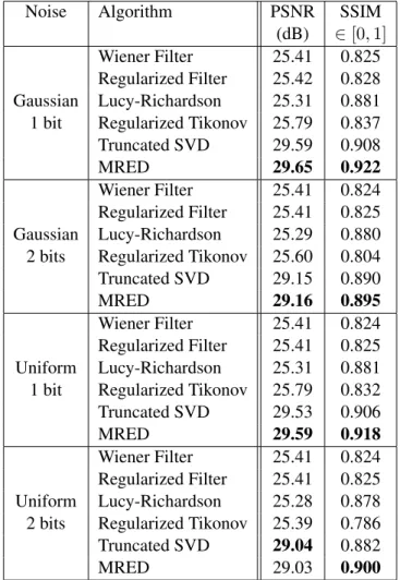
3.1 Image quality measures with different algorithm and different noise statistics . . . 30
3.2 Comparison of different algorithms with different noise mixtures. 34 6.1 PSNR results for Lena and Boat. . . 91
6.2 PSNR results for Napoli. . . 92
6.3 PSNR and detection results in terms of number of identified fea-tures for Target. . . 95
6.4 ENL for real SAR images. . . 99
D.1 Parameters setting for the PCkNN algorithm . . . 131
D.2 PSNR (dB) results for the test images. . . 133
D.3 Tab. D.2 (continued). PSNR (dB) results for the test images. . . . 134
D.4 SSIM (∈ [0, 1]) results for the test images. . . 135
D.5 Tab. D.4 (continued). SSIM (∈ [0, 1]) results for the test images. . 136
Chapter 1
Introduction
The general context of this thesis is the Image Restoration. Part of the work pre-sented here has been developed at the Napoli University. Indeed, my Ph.D. pro-gram has been developed between the University of Napoli “Federico II” (Italy) and the University of Nice-Sophia Antipolis (France), in the framework of a co-tutelle doctoral project. The topic I spent most of the time on, has been AWGN image denoising, at the University of Nice, while my time at University of Napoli was focused on application to SAR image denoising.
1.1 Context
Algorithms of image processing and computer vision can be classified in three main categories: low-level, mid-level and high-level algorithms. Low-level algo-rithms process basic operations on image pixels, e.g., some pixels are moving in the image plane. Mid-level vision includes higher level processing like pixel group-ing. High-level vision is the final stage which gives a semantic meaning to the scene. This document deals with low-level image processing tasks that may rep-resent building bricks for content analysis or understanding. Mainly two problems will be studied: deconvolution and denoising. Image inpainting, will be briefly mentioned.
A central notion in this kind of problems is the notion of similarity. Many image and video processing problems can be solved by optimizing some cost func-tions. The notion of similarity is often behind these funcfunc-tions. It can be a self-similarity when a coherence is searched for within an object, or a cross-self-similarity between two objects, images, or videos. Image restoration and segmentation typi-cally call upon self-similarity and content-based indexing and retrieval depend on the definition of a cross-similarity. Intermediately, tasks performed on video such as restoration, segmentation, tracking, and optical flow computation rely upon a similarity of an objet or a scene view with itself as observed on another frame.
1.2 Contributions of the thesis
The main contribution of this thesis is a new statistical framework inspired from Information Theory to address the problem of image restoration. Many problems of image and video processing can be expressed as the minimization of a data con-sistency residual and a term of mismatch with respect to a priori constraints. Tra-ditionally, these functionals are based on penalization functions such as the ones defined for robust estimation, sometimes referred to as φ-functions. From a statis-tical point of view, recurring to these functions is equivalent to implicitly making assumptions on the probability density functions (PDFs) of the residual and the model mismatch, e.g., Gaussian, Laplacian, or other parametric laws for the square function, the absolute value, or other φ-functions, respectively. Alternatively, it is interesting to adapt to (an estimation of) the true PDF. This nonparametric ap-proach implies to define functionals which take PDFs as input. Entropy has been proposed in this context since, as a measure of dispersion of a PDF, its minimiza-tion leads the residual or model mismatch values to concentrate around narrow modes, the highest one normally corresponding to the annihilation of the residual or mismatch, the others corresponding to inevitable outliers.
Based on this considerations, a novel method for image deconvolution based on the minimization of the residual entropy has been proposed in the first part of this thesis. The use of entropy turns out to be robust with respect to different noise distributions applied to the observations. Indeed, the only hypothesis on the noise is the spatial independency, i.e., noise samples in different spatial location are statistical independent.
In the same spirit of this Information Theory-driven approach the denoising problem has been tackled in the second part of the thesis. Here, we rely on the notion of patch, i.e., a portion (usually a small square) of the image. Then the patch conditional entropy, which carries the residual information of the central pixel knowing its neighborhood, is considered. The denoising is performed in or-der to reduce this conditional entropy which has been leveled up by the presence of the noise. Developing this model leads to an information based interpretation of state of the art patch based denoising algorithms. Indeed, the derivation of the entropy criterion leads to a (weighted) average (or equivalently a filtering) of sim-ilar patches. This step is the core of state-of-the-art algorithms such as NLmeans and BM3D. Although the minimization of the conditional entropy has been intro-duced in UINTA, we proposed a different minimization scheme in the space of the patches coupled with the aggregation (or reprojection) step from the BM3D strategy.
The third part of this thesis deals with specific application of the denoising technique. In particular, in Chapter 5 we apply the denoising procedure developed in Chapter 4 to professional real world camera image. In this kind of images the noise can be considered still Gaussian, but signal dependent. Indeed the variance of the noise can be modeled as an affine function of the signal intensity. Furthermore, modern camera sensors produce RAW images which are mosaiced. This means
1.2. CONTRIBUTIONS OF THE THESIS 3 that in each spatial position (or pixel), only one color information is available. To have a complete RGB image a further step, called demosaicing, is required. This step combines the outputs of neighbors pixel in order to reconstruct the R,G, and B components in each spatial position. Denoising can be performed before or after the demosaicing step. However, demosaicing introduces correlation among neighborhood pixels and hence correlates the noise. The result is a “structured noise” which is not Gaussian and not independent anymore. Removing this noise is a harder task since algorithms usually rely on a hypothesis of independence. Therefore, denoising is performed before demosaicing. The algorithm has been then adapted in order to deal with the variable variance of the noise ant the complex geometry of CFA matrix.
Chapter 6 presents a denoising scheme for Synthetic Aperture Radar (SAR) images which adapts the BM3D algorithm to SAR images peculiarities such as the multiplicative noise. This part of the work has been developed at the University of Naples. Although not stated in the variational framework, this scheme belongs to the general patch-based denoising context. The image self-similarity is exploited in order to filter the noise while preserving textures and edges.
Finally, Chapter 7 deals with the problem of digital image inpainting, which represents a growing area of image processing and computer vision research. Briefly, we adapted the denoising AWGN method in order to fill the dam-aged/missing regions in the image.
Chapter 2
ESTIMATION OF SOME
STATISTICAL MEASURES
2.1 Introduction
The solution to image and video processing problems can often be formulated as follows
ˆ
x = arg min
x φd(y− Hx) + λφr(∇x) (2.1)
where φd (usually the Lp-norm operator) and φr correspond to data fidelity and
regularization, respectively, and λ is the regularization parameter. Under some hy-pothesis one can note that (2.1) corresponds to the Maximum A Posteriori solution if the noise follows a generalized Gaussian law of shape parameter p and the a pri-ori on the solution is given by a Gibbs PDF. These laws being defined by a small number of parameters, (2.1) can only adapt to the data to a limited extent. More-over, such parametric assumptions may not be flexible enough to efficiently deal with outliers.
Even if one can pick functions proposed in robust estimation in order to reduce the bias introduced by outliers, these functions are still sensitive to the values of the outliers nonetheless. Moreover, they still represent an implicit assumption on the underlying distribution of the data.
On the contrary entropy and other related statistical measures are less sensitive to outliers because they deal with them in terms of frequency of occurrence as opposed to value. In addition, if the PDF(s) is/are estimated nonparametrically, then the measure makes no assumptions on the data or, otherwise stated, adapts to them.
In this chapter we resume the basics of nonparametric estimation of some sta-tistical measures focusing on the k-Nearest Neighbors (kNN) framework which presents a lot of advantages in dealing with high dimensional spaces.
2.2 Kernel density estimation (KDE)
Kernel-based methods make no assumption about the actual PDF. Consequently, the estimated PDF cannot be described in terms of a small set of parameters, as opposed to, e.g., a Gaussian PDF defined by its mean and variance. Such method are then qualified as non-parametric. KDE is an important class of estimators since virtually all nonparametric algorithms are asymptotically kernel methods [TS92].
Let {s1, s2, . . . , sn} be a set of n independent observations of a random
vari-able X with p(·) as PDF. The basic KDE may be written compactly as ˆ p(s) = 1 nh n � i=1 K � s− si h � = 1 n n � i=1 Kh(s− si), (2.2)
where Kh(t) = K(t/h)/h. Thus a kernel estimator is an equal mixture of n
kernels, centered at the n data points.
Choosing a good value for the bandwidth, h, is the most difficult task. The choice of this parameter will be further discussed in Section2.2.2
2.2.1 Multivariate KDE
The extension of the kernel estimator to the multivariate case where the samples are vector-valued data, s ∈ Rd, is straightforward, The KDE ˆp uses the multivariate
d-dimensional kernels KH(·), where the bandwidth H is a d×d covariance matrix.
Therefore Eq.(2.2) writes ˆ p(s) = 1 n n � i=1 KH(s− si), (2.3)
where, in the most general case, KH(s) = |H|−1/2K(H−1/2s), with H being
a d × d symmetric and positive definite bandwidth matrix, whose meaning will be clarified later, and K(·) being a d-variate kernel function, bounded and with compact support, satisfying the following set of conditions [WJ95]:
� Rd K(s)ds = 1, lim ||s||→∞||s|| dK(s) = 0, � Rd sK(s)ds = 0, � Rd ssTK(s)ds = cKI, (2.4)
where cK is a constant and I is the identity matrix. It is convenient to separate
the size of H from the orientation of H. To that end, write H = h2A, where
det A = 1. Thus, the size of H is det h2A = h2d. Commonly data are rotated
by the transformation A−1/2, then a normal kernel or, more generally, a product
kernel, possibly with different smoothing parameter, hk, in the k-direction:
ˆ p(s) = 1 n n � i=1 � d � k=1 Khk(s (k) − s(k)i ) � . (2.5)
2.2. KERNEL DENSITY ESTIMATION (KDE) 7
2.2.2 Bandwidth selection
As mentioned before, the critical parameter of KDE is the bandwidth h. In practice as long as in theory, this parameter should tend to zero when the number of samples tends to infinity. Larger bandwidth will capture overall structure while smaller bandwidth will get finer structure.
The problem of an automatic, data-driven choice of the bandwidth has actually more importance for the multivariate than for the univariate case. In one or two dimensions one can choose an appropriate bandwidth interactively just by look-ing at the plot of density estimates for different bandwidths. However, this task becomes very hard, if not impossible, in dimensions higher than 3. Two of the most frequently used methods of bandwidth selection are the plug-in method and the method of cross-validation, which can make the selection of this parameter automatic. Among the plug-in rules we recall here:
• a Parzen bandwidth selection is the Silverman’ rule-of -thumb [Sil86] ˆ
h≈ 1.06ˆσn−1/5, (2.6)
where ˆσ is an estimation of the unknown density standard deviation. ˆ σ = � � � � 1 n− 1 n � i=1 (si− ¯s)2. (2.7)
• In the multivariate case, it is not possible to derive the rule-of-thumb for general H and Σ. However, if we consider H and Σ to be diagonal matrices,
ˆ hj = � 4 d + 2 �1/(d+4) n−1/(d+4)σj. (2.8)
Note that this formula coincides with Silverman’s rule of thumb in the case d = 1, see (2.6) and [Sil86]. Replacing the σjs with estimates and noting
that the first factor is always between 0.924 and 1.059, we arrive at Scott’s rule [Sco92]:
ˆ
hj = ˆσjn−1/d+4. (2.9)
Equation (2.8) shows that it might be a good idea to choose the bandwidth matrix H proportional to Σ−1/2, where Σ is the covariance matrix of the
data. In this case we get as a generalization of Scott’s rule ˆ
H = n−1/(d+4)Σˆ−1/2. (2.10) Using such a bandwidth corresponds to a transformation of the data, so that they have an identity covariance matrix. As a consequence we can use band-width matrices to adjust for correlation between the components of X . Another method for automatic bandwidth selection is the double kernel esti-mates, which estimates the density with two different kernels (e. g., Gaussian and Epanechnikov) and tries to find the bandwidth which minimizes the distance be-tween these two estimation.
Figure 2.1: Kernel density estimation performance on a 1-D Gaussian mixtures for different bandwidth. Actual distribution is in black, kernel density estimate is in blue and kernels are in red. h is the plugin estimate using rule of thumb, from left to right, top to bottom: actual PDF, PDF estimated with 0.2h, PDF estimated with h, PDF estimated with 5h.
2.2. KERNEL DENSITY ESTIMATION (KDE) 9
Figure 2.2: Multivariate kernel density estimation performance on a 2-D Gaussian mixtures for different bandwidth. h is the plugin estimate using rule of thumb, from left to right, top to bottom: actual PDF, PDF estimated with 0.2h, PDF estimated with h, PDF estimated with 5h.
2.3 Nonparametric entropy estimation
Entropy is a functional of the PDF and represents a measure of dispersion of a random variable. The differential entropy H(pX), or equivalently H(X), of a
continuous random variable X of Rdwith PDF p, writes
H(X) =− �
Rd
p(α) log p(α)dα. (2.11)
2.3.1 Plug-in estimates
The plug-in estimates of entropy are based on a consistent density estimate pnof p
such that pndepends on X1, . . . , Xn.
Integral estimate
The integral estimator is of the form Hn=−
�
An
pn(t) log pn(t)dt, (2.12)
where, with the set Anone typically excludes the small or tail values of pn. This
estimator was first proposed by Dimitriev and Tarasenko [DT74], who proved the strong consistency of Hnfor d = 1. The evaluation of the integral in (2.12)
how-ever requires numerical integration and is not easy if pn is a KDE. Joe [Joe89]
considers estimating H(p) by (2.12) when p is a multivariate PDF, but he points out that the calculation of (2.12) when pnis a KDE gets more difficult for d ≥ 2.
The resubstitution estimate
Ahmad and Lin [AL76] proposed estimating H(p) by Hn=− 1 n n � i=1 log pn(Xi), (2.13)
where pnis a kernel density estimate. They showed the mean square consistency
of (2.13) for d = 1. Joe [Joe89] considered the estimation of H(f) for multivariate PDF’s by an entropy estimate of the resubstitution type2.13, also based on a KDE. His analysis and simulations suggest that the sample size needed for good estimates increases rapidly with the dimension d of the multivariate density.
2.3.2 The kNN framework
A consistent and unbiased entropy estimator was proposed for k = 1 [KL87]. This work was extended to k ≥ 1 with a proof of consistency under weak conditions on
2.4. ENTROPY DERIVATIVE AND MEAN SHIFT 11 the underlying PDF [GLMI05]
HkN N(U ) = log(vd(|U| − 1)) − ψ(k) + d |U| � s∈U log ρk(U, s), (2.14)
where vdis the volume of the unit ball in Rd, |U| is the cardinality of the sample set
U, ψ is the digamma function Γ�/Γ, and ρk(U, s)is the distance to the k-th nearest
neighbor of s in U excluding the sample located at s if any. Informally the main term in estimate (2.14) is equal to the mean of the log-distances to the k-t nearest neighbor of each sample. Note that (2.14) does not depend on the PDF pU.
While the kNN PDF estimator is competitive in high dimensions only, the en-tropy estimator is accurate even in the univariate case [GLMI05] as shown in Fi-gure2.3.2for several noise distribution. This might be explained by the smoothing effect of the log-distance averaging in (2.14). Moreover, the kNN entropy esti-mator also seems reasonably stable with respect to k until fairly high dimensions. Therefore, the choice of k does not appear to be really crucial, as opposed to the choice of h in the Parzen method. Actually, k must tend toward infinity when |U| tends toward infinity, and such that k/|U| tends toward zero when |U| tends toward infinity. An admissible choice is k =�|U|.
2.4 Entropy derivative and Mean Shift
As mentioned in Section2.1, a lot of image processing problems can be formulated as variational: a cost functional, often called energy, is minimized with respect to the unknowns of the problem in order to find a best solution. The minimization procedure often involves the calculus of the energy derivative. When the energy is entropy-based, the gradient of a PDF over the PDF (sometimes called normalized density gradient)
∇p
p =∇log p (2.15)
will be needed. PDFs have either a finite support or they tend toward zero at in-finities, hence the question of stability or even existence of (2.15). Fortunately, this term can be approximated by the Mean Shift vector.
Mean Shift was first introduced in 1975 by Fukunaga and Hoestler [FH75] as a technique for the estimation of probability density gradients, but recently [CM02,
Che95,KF99,LK06] the advantages of such approach both in density estimation and clustering have been newly recognized.
As for the non-parametric density estimation techniques, the main idea on which this approach is based lies on the fact that samples in an arbitrary feature space can be seen as an empirical probability density function, that is, local max-ima of the probability should be observed in areas that have a dense concentration of data points.
The basic approach in the Parzen Window technique lies on the observation that, given a d-dimensional feature space and a set of n data points (s1, . . . , sn),
the probability density function p(s) can be estimated as ˆ pH,K(s) = 1 n n � i=1 KH(s− si), (2.16)
In [CM02], the authors pointed out that a family of kernel functions satisfying the conditions2.4and showing the sufficient property of radial symmetry can be obtained in the following way:
K(s) = ck,dk(�s�2), (2.17)
with ck,d normalizing constant, that is to say defining a univariate kernel profile
k(x)for x ≥ 0 and rotating it in the space Rd. It is further observed in [WJ95]
that, in order to limit complexity in the density estimation procedure, a common practical choice is to set the bandwidth matrix H as proportional to the identity matrix, that is H = h2I, so that only one parameter should be provided in advance.
Under this assumption, the formula of the estimator given in (2.16) becomes ˆ ph,K(s) = ck,d nhd n � i=1 k ��� � � s− si h � � � � 2� (2.18) Applying the gradient operator to both sides of (2.18) yields to the form of the density gradient estimator. Using g(x) = −k�(x), we obtain
ˆ ∇ph,K(s) = 2ck,d nhd+2 n � i=1 (si− s)g ��� � � s− si h � � � � 2� (2.19) = 2ck,d nhd+2 � n � i=1 g ��� � � s− si h � � � � 2�� �n i=1sig ���s−si h � �2� �n i=1g ���s−si h � �2� − s . Observe that the density estimate ˆp(s) evaluated using the function G(s) = cg,dg(�s�2)as a kernel (also called the shadow of kernel K(s)) is given by
ˆ ph,G(s) = cg,d nhd n � i=1 g ��� � �s− sh i � � � � 2� , (2.20)
Therefore it is possible to rewrite Eq. (2.19) as ˆ ∇ph,K(s) = 2ck,d h2c g,d ˆ ph,G(s)mh,G(s), (2.21)
with the term
mh,G(s) = �n i=1sig ���s−si h � �2� �n i=1g ���s−si h � �2� − s , (2.22)
2.5. MEAN-SHIFT APPROXIMATION 13 being called the mean shift (MS) vector. Combining (2.21) and (2.22) we obtain an estimation of the normalized PDF gradient
∇p(s) p(s) ∝ �n i=1sig ���s−si h � �2� �n i=1g ���s−si h � �2� − s . (2.23)
2.5 Mean-Shift approximation
2.5.1 Based on fixed kernel size
As shown in eq. (2.22), the MS vector in the point s involves a weighted average of samples si in the neighborhood of s. The size of the neighborhood depends
on the bandwidth parameter h while the weights are given by the shadow g(·). In the Parzen Window approach (i.e., fixed bandwidth) it can be expressed, using an Epanechnikov [Epa69] kernel k (and hence its shadow g(·) = rect(·)), as
∇p(s) p(s) = d + 2 h2 1 k(s, h) � sj∈Sh(s) (sj− s), (2.24)
where d is the dimension of the feature space S, Sh(s)is the support of the Parzen
kernel centered at point s and of constant size h, k(s, h) being the number of observation falling into Sh(s). The choice of the kernel window size h is
criti-cal [Sco92]. If h is too large, the estimate will suffer from too little resolution, otherwise if h is too small, the estimate will suffer from too much statistical vari-ability. As the dimension of the data space increases, the space sampling gets sparser (problem known as the curse of dimensionality). Therefore, less samples fall into the Parzen window centered on each sample, making the PDF estimation less reliable. Dilating the Parzen window does not solve this problem since it leads to over-smoothing the PDF. In a way, the limitations of the Parzen Method come from the fixed window size: the method cannot adapt to the local sample density. The k-th nearest neighbor (kNN) framework provides an advantageous alternative.
2.5.2 Based on variable kernel size
k-th Nearest Neighbors
Taking the kernel K(·) to be a uniform density on the unit sphere with H(s) = ρk(s)Idwhere ρk(s)is the distance from s to the k-th nearest data point, one has
the k-nearest neighbor estimator [LQ65] (kNN). In the Parzen-window approach, the PDF at sample s is related to the number of samples falling into a window of fixed size centered on the sample. The kNN method is the dual approach: the density is related to the size of the window necessary to include the k nearest neighbors of the sample. Thus, this estimator tries to incorporate larger bandwidths in the tails of the distributions, where data are scarce.
In kNN framework, the MS vector is given by [FH75] ∇p(s) p(s) = d + 2 ρ2 k 1 k � sj∈Sρk sj − s , (2.25)
where ρkis the distance of s to the k-th nearest neighbor.
The kNN estimator is not guaranteed to one (hence, the kernel is not a density) and the discontinuous nature of the bandwidth function manifests directly into dis-continuities in the resulting estimate. Furthermore, the estimator has severe bias problems, particularly in the tails [Hal83,MR79] although it seems to perform well in higher dimension [TS92].
Adaptive Weighted kNN Approach
The kNN method provides several advantages with respect to the Parzen Window method. For example, the number of samples falling in the window is fixed and known. Thus even if the sampling space gets sparser, we cannot have empty re-gions, i.e., no samples inside. Moreover, the window size is locally adaptive. How-ever, as near the distribution modes there is an high density of samples, the window size associate to the k-th nearest neighbor could be too small. In this case the esti-mate will be sensible to statistical variations in the distribution.
To avoid this problem we would increase the number of nearest neighbors, to have an appropriate window size near the modes. However this choice would produce a window too large in the tails of the distribution. Thus very far samples would contribute to the estimation, producing severe bias problems.
We propose an alternative solution that keeps advantages from both Parzen and kNN approaches. The samples contribution is weighted by formally making the following substitution 1 k � sj∈Sρk sj → 1 �k j=1wj k � j=1 sj∈Sρk wjsj. (2.26)
Intuitively, the weights wjmust be a function of distance between the actual sample
and the jth nearest neighbor, i.e., samples with smaller distance are weighted more heavily than ones with larger distance.
2.6 Conclusion
In this chapter we resumed the basics of non parametric estimation. In particular we pointed out that the normalized gradient of a PDF, which often needs to be calculated in entropy-based variational problems, can be locally approximated by means of a weighted average of samples falling in a local neighborhood. In addi-tion we pointed out that the kNN framework easily adapts the neighborhood size
2.6. CONCLUSION 15 Manifold Theoretical Hmanif old HkN N
Plane 2.0 2.0 -3.9
Circle 1.0 1.0 -5.0
Swiss roll 10.6 10.6 8.9
Ring torus 9.6 9.6 7.4
Sphere 5.7 5.2 1.0
Table 2.1: Estimation of Differential Entropy from 3D data embedded on 2D manifolds. Data are uniformely distributed on manifolds. Therefore entropy is log2S, where S is the manifold surface. Nsample = 5000,
Nc = 10and k = 1.
to the local data density and provides more reliable results than a Parzen window approach for high dimensional feature spaces.
Finally, we want to point out that even if standard non parametric estimation tools provide very good estimates for ordinary distributions, they can fail if data are complexly structured. This is the case of high dimensional data embedded on lower dimensional manifolds. A novel technique for this kind of data has been proposed in [NK07]. An illustrative example is given in Figure2.6, where 3D data are uniformly distributed on 2D manifold. The theoretical entropy of such a data is, in bits, log2(S), where S is the surface of the manifold. Table2.6shows estimated
Figure 2.3: Entropy estimation of different PDF with relative errors. Cir-cles represent Parzen, i.e. fixed bandwidth, estimation. Squares represent kNN estimator (k = 10) and triangles represent the estimator presented in [NK07].
2.6. CONCLUSION 17
Figure 2.4: 3D data uniformely distributed on embedded 2D manifolds. In lexicographic order: Plane, Spherical surface, Circle (intersection between the Plane and a sphere), Ring torus and Swiss roll. Estimated entropies are given in Table2.6.
Part I
Deconvolution
Chapter 3
ENTROPY-BASED
DECONVOLUTION
3.1 Introduction
Image restoration attempts to reconstruct or recover an image that has been de-graded by using a priori knowledge of the degradation phenomenon. The problem consists in the reconstruction of an original image x from an observed image y. The simplest model connecting x to y is the linear degradation model
y = Hx + n, (3.1)
where H is a linear operator and n is the observation noise. When the operator H is space-invariant the model becomes
y = m∗ x + n, (3.2)
where degradations are modeled as being the result of convolution together with an additive noise term, so the expression image deconvolution (or deblurring) is used frequently to signify linear image restoration [GW02]. Here m represents a known space-invariant blur kernel (point spread function, PSF), x is an ideal version of the observed image y and n is (usually Gaussian) noise.
The objective of restoration is to obtain an estimate ˆx as close as possible to the original image, by means of a certain criterion. We focus on variational methods, that have an important role in modern image research. Classically, the solution minimizes a certain functional, often called energy, which typically is the norm of the residual with some regularization term,
ˆ x = arg min x ||y − Hx|| 2 Σ � �� � Data-fidelity + Jχ(x) � �� � Regularization , (3.3)
where Σ and χ represent two suitable functional spaces. 21
The data-fidelity term measures a sort of distance between the observed and the reconstructed image, while the regularization term describes some properties (or constraints) of the image we are looking for. In stochastic based approaches, x, yand n are considered as realizations of random fields.
In this chapter, we develop a new deconvolution algorithm which minimizes the residual differential entropy.
3.2 State of the art
3.2.1 Deterministic approach
We consider a space-invariant imaging system, such that the model of image for-mation is given by1
y(u) = �
m(u− v)x0(v)dv + n(u). (3.4)
Inverse filter
Suppose for simplicity that the signal-to-noise ratio (SNR) is sufficiently large such that we can reasonably neglect at first sight the noise term in eq.(3.4). If we use the Fourier transform (FT), eq.(3.4) becomes rather trivial since we get
Y (f ) = M (f )X0(f ). (3.5)
It is clear from equation(3.5) that the support of M(f) plays an important role in the solution of the problem. Indeed, the uniqueness of the solution is closely related to the null space of the convolution operator, i.e. the solution of the equation
M (f )X(f ) = 0. (3.6)
If the support of M(f) is the whole frequency space, then X(f) = 0. In this case the solution of the restoration problem is unique and is given by
X(f ) = Y (f )
M (f ). (3.7)
However if we are in the presence of noise we get X(f ) = X0(f ) +
N (f )
M (f ). (3.8)
The second term in equation(3.8) comes from the inversion of the noise contribu-tion and it may be responsible for the non-existence of the solucontribu-tion. Indeed since the noise is a process independent of the image formation, there may be division
3.2. STATE OF THE ART 23 by zero and X(f) has singularities at the zeros of M(f). Moreover, even if M(f) is not zero for some values of f, it tends to be zero when |f| → ∞. Since the be-havior of N(f) is not related to M(f), the ratio N(f)/M(f) may not tend to zero. Hence, the solution may not exist or be not stable due to the noise amplification.
On the other hand, if the support of M(f) is a bounded subset of the frequency space, the solution of the image deconvolution problem is not unique. In this case we take as solution the least-squares (LS) solution.
Wiener filter
The inverse filter divides in the frequency domain by numbers that are very small, which amplifies any observation noise in the image. A better approach is based on the Wiener filter [Wie49]. The goal is to find a filter which gives an estimate ˆ
x = g∗ y such that it minimizes the mean square error. In the Fourier domain, the Wiener filter is given by
G(f ) = M∗(f )Sx(f ) |M(f)|2S
x(f ) + Sn(f )
, (3.9)
where Sx(·) and Sn(·) are the mean power spectral density of the input signal x(·)
and the noise n(·) respectively.
The operation of the Wiener filter becomes apparent when the filter equation above is rewritten: G(f ) = 1 M (f ) � |M(f)|2 |M(f)|2+ SN R−1(f ) � , (3.10)
where SNR(f) = Sx(f )/Sn(f )is the signal-to-noise ratio. When there is zero
noise (i.e. infinite signal-to-noise), the term inside the square brackets equals 1, which means that the Wiener filter is simply the inverse of the system, as we might expect. However, as the noise at certain frequencies increases, the signal-to-noise ratio drops, so the term inside the square brackets also drops. This means that the Wiener filter attenuates frequencies dependent on their signal-to-noise ratio. The Wiener filter equation above requires us to know the spectral content of a typical image, and also that of the noise. Often, we do not have access to these exact quantities, but we may be in a situation where good estimates can be made. For instance, in the case of photographic images, the signal (the original image) typically has strong low frequencies and weak high frequencies, and in many cases the noise content will be relatively flat with frequency.
3.2.2 Statistical methods
As opposed to deterministic approaches which do not take into account the random nature of noise, in stochastic approaches y, x, and n are considered as realization of random fields. If some statistical property of the noise, such as the expecta-tion value or the correlaexpecta-tion funcexpecta-tion or the probability distribuexpecta-tion, is known,
then one can develop methods where this information is used for image decon-volution. In classical statistics, Maximum Likelihood (ML) is the most commonly used method for parameter estimation. Its application to image restoration is based on the knowledge of the random properties of noise so that the probability den-sity pn(y|x) is known. Then the ML estimator looks for the image x which is
most likely to produce the detected image y, i. e. the image which maximize the probability of observing y
max
x p(y|x) (3.11)
with p(y|x) = p(y = Mx + n|x) = p(n = y − Mx). If the noise is white and gaussian, pN(t) = 2πσ1 exp−||t|| 2 2σ2 and max x p(y|x) = maxx 1 2πσexp− ||y − Mx||2 2σ2 ⇔ minx ||y − Mx|| 2. (3.12)
Thus, in the case of additive Gaussian noise, the ML-method is equivalent to the LS method.
3.2.3 Why using entropy?
As it is well known, LS estimation is sensitive to outliers, or deviations, from the assumed statistical model. In the literature other more robust estimators have been proposed, like M-estimators [BA93], involving quadratic and possibly non-convex energy functions. However, these methods rely on parametric assumptions on the noise statistics, which may be inappropriate in some applications due to the contribution of multiple error source, such as radiometric noise (Poisson), readout noise (Gaussian), quantization noise (Uniform) and ”geometric” noise, the latter due to the non-exact knowledge of the PSF. Therefore density estimation using a nonparametric approach is a promising technique.
We propose to minimize a functional of the residual distribution, in particu-lar the differential entropy of the residual. We use entropy because it provides a measure of the dispersion of the residual, in particular low entropy implies that the random variable is confined to a small effective volume and high entropy indicates that the random variable is widely dispersed [CT91]. Moreover, entropy criterion is robust to the presence of outliers in the samples. Experimental results with non gaussian distributions show the interest of such a nonparametric approach.
3.3 Proposed method: MRED
3.3.1 Minimizing the residual entropy
Image deblurring is an inverse problem, that can be formulated as a functional minimization problem. Let Ω denote a rectangular domain in R2, on which the
3.3. PROPOSED METHOD: MRED 25 Ideally, the recovered image ˆx satisfies
ˆ x = arg min x � Ω ϕ(y− m ∗ x) du, (3.13)
where ϕ(·) is a metric representing data-fidelity. In the case of Gaussian noise, a quadratic function is used. However, parametric assumptions on the underly-ing noise density function are not always suitable, due to the multiple source of noise. We define as energy to be minimized a continuous version of the Ahmad-Lin [AL76] entropy estimator (HA−L(r)), defined as:
E(x) = |Ω| HA−L(r)
= −
�
Ω
log(px(r(u)))du . (3.14)
In order to solve the optimization problem a steepest descent method is used. The energy derivative has been analytically calculated and it is shown in section3.3.3.
3.3.2 Energy lower bound
In this section we provide a lower bound (LB) to the energy in eq.(3.14), in order to check how our algorithm works on minimizing residual entropy (see Fig.3.1). The residual can be viewed as the sum of two random variables, namely, R = N + ˜X. The first one is the noise, and the second one is the projection of the error by means of the operator m(·), i.e., ˜x = m ∗ (x0− x).
Proposition 3.1. The residual entropy h(R) is lower bounded by the noise entropy h(N ).
Proof. Let us consider the mutual information between R and ˜X, I(R; ˜X) = h(R)− h(R| ˜X)
= h(R)− h(N| ˜X) .
Since the noise N is independent from ˜X, h(N| ˜X) = h(N ), and by the non negativity property of mutual information we obtain
h(R)≥ h(N) . (3.15)
As it is well known, mutual information is a measure of the amount of infor-mation that one random variable contains about another random variable [CT91]. The closer x is to the original image x0, the less information on ˜Xis carried by the
residual. Therefore entropy minimization can be interpreted as the process which uses the information carried by the residual to recover x0, until there is no more
0 1 2 3 4 5 6 0 1 2 3 4 5 6
Noise Differential Entropy (bits)
bits Initial Entropy Final Entropy Lower Bound 0 1 2 3 4 5 6 0 1 2 3 4 5 6
Noise Differential Entropy (bits)
bits
Initial Entropy Final Entropy Lower Bound
a) Gaussian Noise b) Uniform Noise
Figure 3.1: Residual Entropy as function of noise entropy.Initial residual entropy (blue), Final residual entropy (green), Theoretical lower bound (red).
3.3.3 Energy derivative
The residual pdf is estimate by using a nonparametric continuous version Parzen estimator, with symmetric kernel K(·),
px(s) = 1 |Ω| � Ω K(s− r(u)) du . (3.16)
Note that px(s) is the residual pdf associated to the current estimate image x.
Therefore changes in x provides changes in px(s), hence changes in the residual
entropy (energy). By taking the Gˆateaux derivative of eq.(3.14) it can be shown (see the AppendixAfor the demonstration.) that the gradient of E(x) at v ∈ Ω is equal to ∇E(x)(v) = � Ω m(v− w) k(w) dw, (3.17) with k(w) = ∇px(r(w)) px(r(w)) + χ(w) (3.18) and χ(w) =− 1 |Ω| � Ω ∇K(r(u) − r(w)) px(r(u)) du . (3.19)
The first term in (3.18) is the normalized gradient of the residual pdf and it is pro-portional to the local Mean-Shift (MS) [FH75]. In the following the MS estimation is addressed as well as the computation of Eq.3.19.
3.4. EXPERIMENTAL RESULTS 27 Mean-Shift approximation
The first term in (3.18) is the normalized gradient of the residual pdf and it is proportional to the local mean-shift [FH75]:
∇px(X)
px(X)
= d + 2
h2 Mh(X), (3.20)
where Mh(X)is the local MS vector. MS estimation can be dealt with either a
Parzen window or a k-th nearest neighbor (kNN) approach. Since the residual is scalar, the Parzen approach is more suitable. Therefore the MS is
Mh(X) = 1 k � Xi∈Sh(X) (Xi− X) (3.21)
i.e., the sample mean shift of the observations in the small region Sh(X)centered
at X (Sh(X) ={Y : �Y − X�2 ≤ h2}).
Second order term χ
The integral in (3.19) is difficult to calculate in the general case and its computation is developed in AppendixB. However, under some hypotheses, the residual pdf is approximatively
px(α)≈ N (α)
|D| , (3.22)
where N(α) is the number of samples such that r(w) = α. Note that, this approx-imation does not make any assumption on the underlying residual pdf. χ(w) is the sample mean of a function of the random variable R, i.e.,
1 |D| � D ∇Kσ(r(u)− r(w)) px(r(u)) du ≈ � suppR∇Kσ (α− r(w)) dα. (3.23) This is function of r(w), if r(w) = 0 and the support of R is symmetric, the value of χ(w) is 0 as long as it is an integral of an even function. By means of this considerations, we could expect a negligible value of χ(w) if r(w) is small, and higher values near the boundary of the support of R.
3.4 Experimental Results
In this section, some results from MRED (Minimum residual Entropy Deconvolu-tion) algorithm are shown and compared to some state-of-the-art techniques: the Wiener filter [Wie49], the Lucy-Richardson [Ric72,Luc74] algorithm, the regular-ized inverse filter, the regularregular-ized Tikonoff filter and the Truncated SVD [HNO06] In order to measure the performance of our algorithm we blurred the Lena image (512x512 pixel) by convolving it with a 13x13 Gaussian PSF with stan-dard deviation√3, and adding noise with different distributions, such as Gaussian,
Uniform, Gaussian mixture, Gaussian-Uniform mixture and with different entropy magnitudes. Residual entropy minimization is carried out via the gradient descent algorithm described in section3.3.3. At each iteration the mean-shift kernel size h is proportional to the standard deviation of the residual, since this choice generally assures a good compromise between robustness and accuracy [Com03].
Figure3.1shows in blue the initial residual entropy in green the value attained when the algorithm converges and in red the theoretical LB. We considered Gaus-sian noise in Figure3.1a and Uniform noise in Figure3.1b. In the gaussian case the proposed algorithm achieves the lower bound of entropy. However, in the uniform case as well the final entropy is quite close to the LB with a maximum relative difference of 0.02%.
The performance is quantified by the Peak Signal-to-Noise Ratio, PSNR = 10 log10|x|
2 max
MSE (3.24)
where |x|max is the maximum value admitted by the data format and the
mean-square error
MSE =�[x(n) − ˆx(n)]2� (3.25) is computed as a spatial average �·�, with x and ˆx being the original and restored images, respectively. We also use a recent novel quality assessment measure: the Structure Similarity (SSIM) index [WBSS04], which proved to be more consistent with the human eye perception. The SSIM measure is calculated between small windows (usually 8 × 8) of an image, namely x and y, as follows,
SSIM(x, y) = � (2µxµy+ c1) (2σxy+ c2) µ2
x+ µ2y+ c1�(σx2+ σ2y+ c2)
, (3.26)
where µ·and σ·represent respectively the image average and the variance in the
window and c1, c2two constants to stabilize the division with weak denominator.
Figure3.2shows the PSNR and SSIM measures between the original image x0
and the degraded image y (blue) and the restored image ˆx (red) in function of the noise entropy for Gaussian and Uniform distribution.
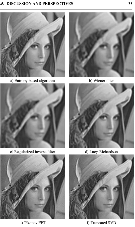
Figure (3.4) shows the restored images from different algorithms as Lucy-Richardson [Ric72,Luc74] and Truncated SVD [HNO06], with uniform noise (en-tropy 2 bits). The truncation parameter of TSVD is found with a generalized cross validation [HNO06]. MRED has roughly the same PSNR of the TSVD restored image, however the latter has a more pronounced grain effect. This is well catched by the SSIM measure, for which our method is considered of higher quality. SSIM indicates better results also in the experiment of Figure3.7, where a gaussian mix-ture noise has been used (see Fig. 3.6), even if the PSNR is lower than the one provided by the TSVD restoration.
A full set of comparisons is shown in Tabb. 3.1 and 3.2 for different noise distributions and entropy values. In particular, Tab.3.2reports results for the two non canonical noise distributions shown in Figure3.6. For the sake of clarity,
3.5. DISCUSSION AND PERSPECTIVES 29 0 1 2 3 4 5 6 18 20 22 24 26 28 30 32 PSNR Gain (dB)
Noise Entropy (bits)
(dB) Final PSNR Initial PSNR 0 1 2 3 4 5 6 0.4 0.5 0.6 0.7 0.8 0.9 1 SSIM Gain
Noise Entropy (bits)
Final SSIM Initial SSIM 0 0.5 1 1.5 2 2.5 3 3.5 25 26 27 28 29 30 31
Noise Entropy (bits)
PSNR (dB) Final PSNR Initial PSNR 0 0.5 1 1.5 2 2.5 3 3.5 0.83 0.84 0.85 0.86 0.87 0.88 0.89 0.9 0.91 0.92 0.93
Noise Entropy (bits)
SSIM Index
Final SSIM Initial SSIM
(a) PSNR (b) SSIM
Figure 3.2: Algorithm performances for gaussian noise (top) and uniform noise (bottom) as function of noise entropy. (a) Initial (blue) and Final (red) PSNR; (b) Initial (blue) and Final (red) SSIM.
the best PSNR and SSIM value is put in boldface. The MRED algorithm always outperforms the other techniques except that in the two aforementioned cases for the PSNR value.
3.5 Discussion and perspectives
In this chapter we presented a deconvolution method in the variational framework based on the residual entropy minimization. We gave a theoretical meaning of the minimization procedure in terms of mutual information between random variables. The simulations indicated robust performance for different non-standard noise dis-tribution probabilities. The robustness comes from the non parametric estimation which makes no assumptions on the noise PDF. Experiments show in many cases slightly better results w.r.t. some popular deblurring techniques. Results are even more promising considering that, contrarily to what happens in other techniques
Noise Algorithm PSNR SSIM (dB) ∈ [0, 1] Wiener Filter 25.41 0.825 Regularized Filter 25.42 0.828 Gaussian Lucy-Richardson 25.31 0.881 1 bit Regularized Tikonov 25.79 0.837 Truncated SVD 29.59 0.908
MRED 29.65 0.922
Wiener Filter 25.41 0.824 Regularized Filter 25.41 0.825 Gaussian Lucy-Richardson 25.29 0.880 2 bits Regularized Tikonov 25.60 0.804 Truncated SVD 29.15 0.890
MRED 29.16 0.895
Wiener Filter 25.41 0.824 Regularized Filter 25.41 0.825 Uniform Lucy-Richardson 25.31 0.881 1 bit Regularized Tikonov 25.79 0.832 Truncated SVD 29.53 0.906
MRED 29.59 0.918
Wiener Filter 25.41 0.824 Regularized Filter 25.41 0.825 Uniform Lucy-Richardson 25.28 0.878 2 bits Regularized Tikonov 25.39 0.786 Truncated SVD 29.04 0.882
MRED 29.03 0.900
Table 3.1: Image quality measures with different algorithm and different noise statistics
3.5. DISCUSSION AND PERSPECTIVES 31 0 20 40 60 80 100 120 140 160 2 2.5 3 3.5 4 4.5 iteration
Residual Entropy (bits)
Figure 3.3: Left: Degraded image with a gaussian filter (σ2 = 3), and
zero mean Uniform noise of entropy 2 bits. Right: Residual entropy as function of iterations.
like Truncated SVD, MRED algorithm makes no use of regularization parameters. In most cases, iterative methods, converging to the ML-solutions, are used in such a way that regularization can be obtained by early stopping of the iterations. In-deed, these methods have the so-called semi-convergence property: the iterates first approach the ”correct” solution and then go away. As future work, a possible regularization method is being taken into account that makes use of the Kullback-Leibler divergence between the residual distribution and the noise model, under the hypothesis that some a priori knowledge is available on the noise. A further remarkable property of MRED is its possible extension to the case of multispectral images.
a) Entropy based algorithm b) Wiener filter
c) Regularized inverse filter d) Lucy-Richardson
e) Tikonov FFT f) Truncated SVD
3.5. DISCUSSION AND PERSPECTIVES 33
a) Entropy based algorithm b) Wiener filter
c) Regularized inverse filter d) Lucy-Richardson
e) Tikonov FFT f) Truncated SVD
Figure 3.5: Deconvoluted images comparison, Gaussian mixture noise, entropy 1.85 bits
Noise Algorithm PSNR SSIM (dB) ∈ [0, 1] Wiener Filter 25.43 0.824 Mixture Regularized Filter 25.41 0.824 Gaussian Lucy-Richardson 25.31 0.879 1.85 bits Regularized Tikonov 25.40 0.785 Truncated SVD 28.93 0.876
MRED 25.94 0.899
Wiener Filter 25.41 0.824 Mixture Regularized Filter 25.41 0.824 Gaussian Lucy-Richardson 25.32 0.881 Uniform Regularized Tikonov 25.63 0.837 0.7 bits Truncated SVD 29.66 0.913
MRED 29.80 0.926
Table 3.2: Comparison of different algorithms with different noise mixtures.
−1 0 1 2 3 4 5 0 500 1000 1500 2000 2500 3000 −2.5 −2 −1.5 −1 −0.5 0 0.5 1 1.5 2 2.5 0 1 2 3 4 5 6 7 8x 10 −3
Figure 3.6: Mixture noise. Left: Gaussian mixture pdf (entropy 1.85 bits). Right: Gaussian/Uniform mixture pdf (entropy 0.7 bits).
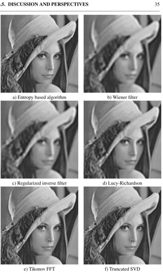
3.5. DISCUSSION AND PERSPECTIVES 35
a) Entropy based algorithm b) Wiener filter
c) Regularized inverse filter d) Lucy-Richardson
e) Tikonov FFT f) Truncated SVD
Figure 3.7: Deconvoluted images comparison, Gaussian + Uniform mix-ture noise, entropy 0.7 bits
Part II
Denoising
Chapter 4
PATCH-BASED DENOISING
4.1 Introduction
The ineffectiveness of many denoising techniques lies in the inadequacy of the model assumed for the image. In fact, the strategy adopted by various algorithms, is based on the assumption that the noise has a flat spectrum and the original image has significant spectral components only at low frequencies. Following this reason-ing, the noise can be suppressed by attenuating the high frequencies while leaving the lower ones. The result produced is unsatisfactory, for several reasons. First, the high frequency signal components are suppressed together with noise, since it is no possible to distinguish them. It follows that the strong discontinuities or edges of objects, being concentrated at high frequencies, are not correctly reconstructed. In addition, the recovered image still contains a residual lowpass filtered noise.
Progress in denoising methods underwent a significant leap forward with non-local, patch-based methods, even compared with wavelet-based denoising and variational approaches calling upon sophisticated regularization. Based on dis-tinct points of view, the methods UINTA [AW06] (Unsupervised, Information-Theoretic, Adaptive Image Filtering) and NL-means [BCM05] (Non Local means) pioneered this field in which BM3D [DFKE07a] (3D transform-domain collabora-tive filtering) represents the latest, “still to be overcome” improvement, at least in terms of the classical performance measure PSNR1(Peak Signal-to-Noise Ratio).
The central idea of this technique is the notion of self-similarity: given a small region of an image, a so-called patch, it is highly probable that other patches in the image are very similar. All these similar patches are degraded by noise. Never-theless, if the noise is independent and identically distributed, then the correlations between them can be used to get rid of the noise.
In this chapter we develop a patch-based denoising algorithm following the stochastic variational approach. The chosen energy is information theory oriented, involving entropy measures on image patches.
1Although this measure is widely used, it is known that it does not always reflect accurately the
visual quality of the denoised (or, more generally, restored) image.