RESEARCH OUTPUTS / RÉSULTATS DE RECHERCHE
Author(s) - Auteur(s) :
Publication date - Date de publication :
Permanent link - Permalien :
Rights / License - Licence de droit d’auteur :
Bibliothèque Universitaire Moretus Plantin
Institutional Repository - Research Portal
Dépôt Institutionnel - Portail de la Recherche
researchportal.unamur.be
University of Namur
The 3D secular dynamics of radial-velocity-detected planetary systems
Volpi, Mara; Roisin, Arnaud; Libert, Anne-Sophie
Published in:
Astronomy and Astrophysics
DOI:
10.1051/0004-6361/201834896 Publication date:
2019
Document Version
Publisher's PDF, also known as Version of record Link to publication
Citation for pulished version (HARVARD):
Volpi, M, Roisin, A & Libert, A-S 2019, 'The 3D secular dynamics of radial-velocity-detected planetary systems',
Astronomy and Astrophysics, vol. 626, no. id.A74, A74. https://doi.org/10.1051/0004-6361/201834896
General rights
Copyright and moral rights for the publications made accessible in the public portal are retained by the authors and/or other copyright owners and it is a condition of accessing publications that users recognise and abide by the legal requirements associated with these rights. • Users may download and print one copy of any publication from the public portal for the purpose of private study or research. • You may not further distribute the material or use it for any profit-making activity or commercial gain
• You may freely distribute the URL identifying the publication in the public portal ?
Take down policy
If you believe that this document breaches copyright please contact us providing details, and we will remove access to the work immediately and investigate your claim.
A&A 626, A74 (2019) https://doi.org/10.1051/0004-6361/201834896 c ESO 2019
Astronomy
&
Astrophysics
The 3D secular dynamics of radial-velocity-detected planetary
systems
Mara Volpi, Arnaud Roisin, and Anne-Sophie Libert
NaXys, Department of Mathematics, University of Namur, Rempart de la Vierge 8, 5000 Namur, Belgium e-mail: [email protected]
Received 17 December 2018/ Accepted 26 April 2019
ABSTRACT
Aims. To date, more than 600 multi-planetary systems have been discovered. Due to the limitations of the detection methods, our
knowledge of the systems is usually far from complete. In particular, for planetary systems discovered with the radial velocity (RV) technique, the inclinations of the orbital planes, and thus the mutual inclinations and planetary masses, are unknown. Our work aims to constrain the spatial configuration of several RV-detected extrasolar systems that are not in a mean-motion resonance.
Methods. Through an analytical study based on a first-order secular Hamiltonian expansion and numerical explorations performed with a chaos detector, we identified ranges of values for the orbital inclinations and the mutual inclinations, which ensure the long-term stability of the system. Our results were validated by comparison with n-body simulations, showing the accuracy of our analytical
approach up to high mutual inclinations (∼70◦
−80◦
).
Results. We find that, given the current estimations for the parameters of the selected systems, long-term regular evolution of the
spatial configurations is observed, for all the systems, (i) at low mutual inclinations (typically less than 35◦
) and (ii) at higher mutual inclinations, preferentially if the system is in a Lidov-Kozai resonance. Indeed, a rapid destabilisation of highly mutually inclined orbits is commonly observed, due to the significant chaos that develops around the stability islands of the Lidov-Kozai resonance. The extent of the Lidov-Kozai resonant region is discussed for ten planetary systems (HD 11506, HD 12661, HD 134987, HD 142, HD 154857, HD 164922, HD 169830, HD 207832, HD 4732, and HD 74156).
Key words. celestial mechanics – planets and satellites: dynamical evolution and stability – methods: analytical – planetary systems
1. Introduction
The number of detected multi-planetary systems continually increases. Despite the rising number of discoveries, our knowl-edge of the physical and orbital parameters of the systems is still partial due to the limitations of the observational techniques. Nevertheless, it is important to acquire a deeper knowledge of the detected extrasolar systems, in particular a more accurate understanding of the architecture of the systems. Regarding the two-planet systems detected via the radial velocity (RV) method, we have fairly precise data about the planetary mass ratio, the semi-major axes, and the eccentricities. However, we have no information either on the orbital inclinations i (i.e. the angles the planetary orbits form with the plane of the sky) – which means that only minimal planetary masses can be inferred – or on the mutual inclination between the planetary orbital planes imut. This
raises questions about possible three-dimensional (3D) config-urations of the detected planetary systems. Let us note that a relevant clue to the possible existence of 3D systems has been provided for υ Andromedae c and d, whose mutual inclination between the orbital planes is estimated to be 30◦(Deitrick et al.
2015).
A few studies on the dynamics of extrasolar systems have been devoted to the 3D problem. Analytical works byMichtchenko et al.(2006),Libert & Henrard (2007), andLibert & Henrard (2008) investigated the secular evolution of 3D exosystems that are not in a mean-motion resonance. They showed that mutu-ally inclined planetary systems can be long-term stable. In par-ticular, these works focused on the analysis of the equilibria
of the 3D planetary three-body problem, showing the genera-tion of stable Lidov-Kozai (LK) equilibria (Lidov 1962;Kozai 1962) through bifurcation from a central equilibrium, which itself becomes unstable at high mutual inclination. Thus, around the sta-bility islands of the LK resonance, which offers a secular phase-protection mechanism and ensures the stability of the system, chaotic motion of the planets occurs, limiting the possible 3D con-figurations of planetary systems.
Using n-body simulations,Libert & Tsiganis(2009) inves-tigated the possibility that five extrasolar two-planet systems, namely υ Andromedae, HD 12661, HD 169830, HD 74156, and HD 155358, are actually in a LK-resonant state for mutual incli-nations in the range [40◦, 60◦]. They showed that the physical and orbital parameters of four of the systems are consistent with a LK-type orbital motion, at some specific values of the mutual inclination, while around 30%−50% of the simulations generally lead to chaotic motion. The work also suggests that the extent of the LK-resonant region varies significantly for each planetary system considered.
Extensive long-term n-body integrations of five hierarchi-cal multi-planetary systems (HD 11964, HD 38529, HD 108874, HD 168443, and HD 190360) were performed byVeras & Ford (2010). They showed a wide variety of dynamical behaviour when assuming different inclinations of the orbital plane with respect to the line of sight and mutual inclinations between the orbital planes. They often reported LK oscillations for stable highly inclined systems.
InDawson & Chiang(2014), the authors presented evidence that several eccentric warm Jupiters discovered with eccentric Article published by EDP Sciences A74, page 1 of10
giant companions are highly mutually inclined (i.e. with a mutual inclination in the range [35◦, 65◦]). For instance, this is
the case of the HD 169830 and HD 74156 systems, which will also be discussed in the present work.
Recently,Volpi et al. (2018) used a reverse KAM method (Kolmogorov 1954;Arnol’d 1963;Moser 1962) to estimate the mutual inclinations of several low-eccentric RV-detected extra-solar systems (HD 141399, HD 143761, and HD 40307). This analytical work addressed the long-term stability of planetary systems in a KAM sense, requiring that the algorithm construct-ing KAM invariant tori is convergent. This demandconstruct-ing condition leads to upper values of the mutual inclinations of the systems close to ∼15◦.
In the spirit of Libert & Tsiganis (2009), the aim of the present work is to determine the possible 3D architectures of RV-detected systems by identifying ranges of values for the mutual inclinations that ensure the long-term stability of the systems. Particular attention will be given to the possibility of the detected extrasolar systems being in a LK-resonant state, since it offers a secular phase-protection mechanism for mutu-ally inclined systems, even though the two orbits may suffer large variations both in eccentricity and inclination. Indeed, the variations occur in a coherent way, such that close approaches do not occur and the system remains stable.
To reduce the number of unknown parameters to take into account, we use an analytical approach, expanding the Hamiltonian of the three-body problem in power series of the eccentricities and inclinations. Being interested in the long-term stability of the system, we consider its secular evolution, averag-ing the Hamiltonian over the fast angles. Thanks to the adoption of the Laplace plane, we can further reduce the expansion to two degrees of freedom. It was shown in previous works (see for exampleLibert & Henrard 2007;Libert & Sansottera 2013) that if the planetary system is far from a mean-motion resonance, the secular approximation at the first order in the masses is accurate enough to describe the evolution of the system. Such an analyt-ical approach is of interest for the present purpose, since, being faster than pure n-body simulations which also consider small-period effects, it allows us to perform an extensive parametric exploration at a reasonable computational cost. Moreover, in the present work we will show that the analytical expansion is highly reliable, fulfilling its task up to high values of the mutual incli-nation.
The goal of the present work is twofold. On the one hand, we study the 3D secular dynamics of ten RV-detected extrasolar sys-tems, identifying for each one the values in the parameter space (imut, i) that induce a LK-resonant behaviour of the system. On
the other hand, through numerical explorations performed with a chaos detector, we identify the ranges of values for which a long-term stability of the orbits is observed, unveiling for each system the extent of the chaotic region around the LK stability islands.
The paper is organised as follows. In Sect. 2, we describe the analytical secular approximation and discuss its accuracy to study the 3D dynamics of planetary systems in Sect. 3, as well as the methodology of our parametric study. The question of possible 3D configurations of RV-detected planetary systems is addressed in Sect. 4. Our results are finally summarised in Sect.5.
2. Analytical secular approximation
We focus on the three-body problem of two exoplanets revolv-ing around a central star. The indexes 0, 1, and 2 refer to the
star, the inner planet, and the outer planet, respectively. Since the total angular momentum vector C is an integral of motion of the problem, we adopt as a reference plane the constant plane orthogonal to C, the so-called Laplace plane. In this plane, the Hamiltonian formulation of the problem no longer depends on the two anglesΩ1andΩ2, but only on their constant difference
Ω1 −Ω2 = π. Thus, thanks to the reduction of the nodes, the
problem is reduced to four degrees of freedom. We adopt the Poincaré variables, Λi= βi√µiai, ξi= p 2Λi r 1 − q 1 − e2i cos ωi, λi= Mi+ ωi, ηi= − p 2Λi r 1 − q 1 − e2i sin ωi, (1)
where a, e, ω, and M refer to the semi-major axis, eccentricity, argument of the pericenter, and mean anomaly, respectively, and with
µi= G(m0+ mi), βi=
m0mi
m0+ mi
, (2)
for i= 1, 2 . Moreover, we consider the parameter D2(as defined
inRobutel 1995) D2=
(Λ1+ Λ2)2− C2
Λ1Λ2
, (3)
which measures the difference between the actual norm of the total angular momentum vector C and the one the system would have if the orbits were circular and coplanar (by definition, D2is
quadratic in eccentricities and inclinations).
We introduce the translation Lj = Λj−Λ∗j, whereΛ∗jis the
value ofΛjfor the observed semi-major axis aj, for j= 1, 2. We
then expand the Hamiltonian in power series of the variables L, ξ, η, and the parameter D2and in Fourier series of λ, as inVolpi
et al.(2018), H(D2, L, λ, ξ, η) = ∞ X j1=1 h(Kep)j 1,0 (L) + ∞ X s=0 ∞ X j1=0 ∞ X j2=0 D2shs; j1, j2(L, λ, ξ, η) , (4) where – h(Kep)j
1,0 is a homogeneous polynomial function of degree j1in L;
– hs; j1, j2is a homogeneous polynomial function of degree j1in L, degree j2in ξ and η, and with coefficients that are
trigono-metric polynomials in λ.
As we are interested in the secular evolution of the system, the Hamiltonian can be averaged over the fast angles,
H(D2, ξ, η) = ORDECC/2 X j=0 Cj,m,nD2j ORDECC− j X m+n=0 ξmηn, (5)
where ORDECC indicates the maximal order in eccentrici-ties considered, here fixed to 12. When the system is far from a mean-motion resonance, such an analytical approach at first order in the masses is accurate enough to describe the secular evolution of extrasolar systems (see for example Libert & Sansottera 2013). The Hamiltonian formulation Eq. (5) has only two degrees of freedom, with the semi-major axes being constant in the secular approach.
M. Volpi et al.: 3D secular dynamics of RV-detected planetary systems
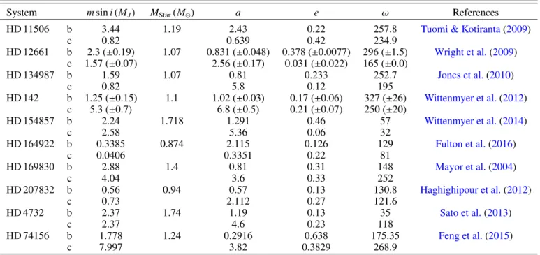
Table 1. Orbital parameters of the selected systems.
System msin i (MJ) MStar(M ) a e ω References
HD 11506 b 3.44 1.19 2.43 0.22 257.8 Tuomi & Kotiranta(2009)
c 0.82 0.639 0.42 234.9 HD 12661 b 2.3 (±0.19) 1.07 0.831 (±0.048) 0.378 (±0.0077) 296 (±1.5) Wright et al.(2009) c 1.57 (±0.07) 2.56 (±0.17) 0.031 (±0.022) 165 (±0.0) HD 134987 b 1.59 1.07 0.81 0.233 252.7 Jones et al.(2010) c 0.82 5.8 0.12 195 HD 142 b 1.25 (±0.15) 1.1 1.02 (±0.03) 0.17 (±0.06) 327 (±26) Wittenmyer et al.(2012) c 5.3 (±0.7) 6.8 (±0.5) 0.21 (±0.07) 250 (±20) HD 154857 b 2.24 1.718 1.291 0.46 57 Wittenmyer et al.(2014) c 2.58 5.36 0.06 32 HD 164922 b 0.3385 0.874 2.115 0.126 129 Fulton et al.(2016) c 0.0406 0.3351 0.22 81 HD 169830 b 2.88 1.4 0.81 0.31 148 Mayor et al.(2004) c 4.04 3.6 0.33 252 HD 207832 b 0.56 0.94 0.57 0.13 130.8 Haghighipour et al.(2012) c 0.73 2.112 0.27 121.6 HD 4732 b 2.37 1.74 1.19 0.13 35 Sato et al.(2013) c 2.37 4.6 0.23 118 HD 74156 b 1.778 1.24 0.2916 0.638 175.35 Feng et al.(2015) c 7.997 3.82 0.3829 268.9 3. Parametric study
In the following, we describe the parametric study carried out in the present work. The selection of the systems considered here is described in Sect.3.1, and the accuracy of the analytical expan-sion for the secular evolution of the selected systems is discussed in Sect.3.2.
3.1. Methodology
The present work aims to identify the possible 3D architectures of RV-detected extrasolar systems. From the online database exoplanets.eu, we selected all the two-planet systems that fulfil the following criteria: (a) the period of the inner planet is longer than 45 days (no tidal effects induced by the star); (b) the semi-major axis of the outer planet is smaller than 10 AU (systems with significant planet–planet interactions); (c) the sys-tem is not close to a mean-motion resonance; (d) the planetary eccentricities are lower than 0.65; (e) the masses of the planets are smaller than 10 MJ. The orbital parameters of the ten selected
systems are listed in Table1, as well as the reference from which they have been derived.
In this work, the secular evolutions of the systems are con-sidered when varying the mutual inclination imut and the orbital
plane inclination i with respect to the plane of the sky. It is impor-tant to note that, although the inclinations i1 and i2 of the two
orbital planes may differ, we decided here to set the same value i for both planes. Thus both masses are varied using the same scaling factor sin i.
In the general reference frame, the following relation holds: cos imut= cos i1cos i2+ sin i1sin i2cos∆Ω, (6)
being∆Ω = Ω1−Ω2. It should be noted that Eq. (6) can be solved
if imut ≤ 2i, thus for a given value of i it determines boundaries
for the compatible values of imut. Since i1 = i2 = i, having fixed
the values of imut, we can determine the value of the longitudes
of the nodes by setting Ω1 = ∆Ω and Ω2 = 0, thus obtaining
the complete set of initial conditions. A consequent change of
coordinates to the Laplace plane is finally performed by using the following relations valid in the Laplace plane:
Λ1 q 1 − e2 1cos iL1+ Λ2 q 1 − e2 2cos iL2= C, Λ1 q 1 − e2 1sin iL1+ Λ2 q 1 − e2 2sin iL2= 0, (7)
where iL1and iL2 denote the orbital inclinations in the
Laplace-plane reference frame.
For our parametric study, we varied the value of the mutual inclination imut from 0◦ to 80◦ with an increasing step of 0.5◦,
while the common orbital plane inclination i runs from 5◦to 90◦ with an increasing step of 5◦. As the coefficients C
j,m,nin Eq. (5)
depend on L, and therefore on the masses of the planets, we recomputed them for each value of i. Regarding the integration of the secular approach, we fixed the integration time to 106yr with an integration step of 1 yr, and the energy preservation was monitored along the integration.
3.2. Accuracy of the analytical approach
Before discussing the results of our parametric study, we need to ensure that the Hamiltonian formulation, Eq. (5), provides an accurate description of the planetary dynamics for all sets of parameters considered in the study, in particular for high val-ues of the mutual inclination imut. As already shown in previous
papers (e.g. Libert & Henrard 2005for the coplanar problem, Libert & Henrard 2007 for the 3D problem), the series of the secular terms converge better than the full perturbation. How-ever, the higher the value of D2, the weaker the convergence,
as expected. In the following, we discuss the numerical conver-gence of the expansion for the selected extrasolar systems, also called convergence au sens des astronomes, as opposed to the mathematical convergence (Poincaré 1893).
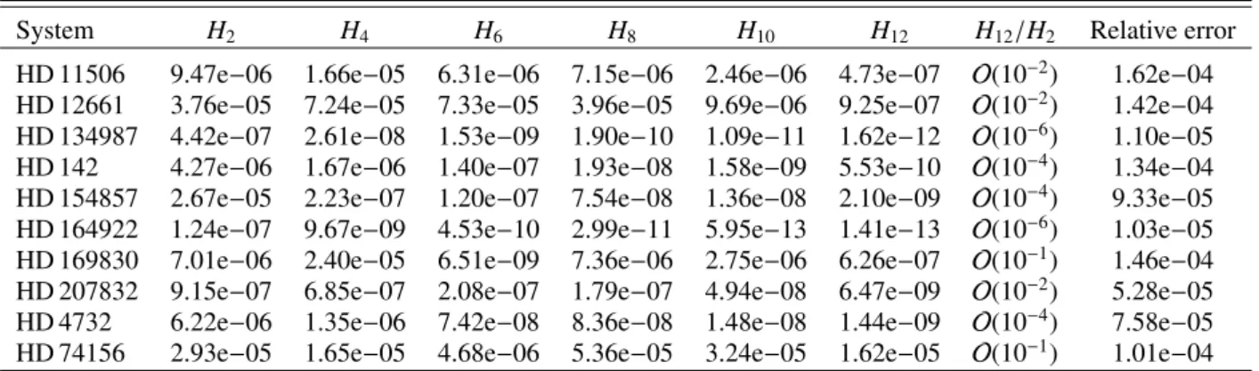
Table 2 lists, for the ten systems, the contributions to the Hamiltonian value of the terms from order 2 to order 12 in eccen-tricities and inclinations (i.e. j+ m + n in Eq. (5)). The entries are
Table 2. Convergence au sens des astronomes for the ten systems.
System H2 H4 H6 H8 H10 H12 H12/H2 Relative error
HD 11506 9.47e−06 1.66e−05 6.31e−06 7.15e−06 2.46e−06 4.73e−07 O(10−2) 1.62e−04 HD 12661 3.76e−05 7.24e−05 7.33e−05 3.96e−05 9.69e−06 9.25e−07 O(10−2) 1.42e−04
HD 134987 4.42e−07 2.61e−08 1.53e−09 1.90e−10 1.09e−11 1.62e−12 O(10−6) 1.10e−05 HD 142 4.27e−06 1.67e−06 1.40e−07 1.93e−08 1.58e−09 5.53e−10 O(10−4) 1.34e−04
HD 154857 2.67e−05 2.23e−07 1.20e−07 7.54e−08 1.36e−08 2.10e−09 O(10−4) 9.33e−05
HD 164922 1.24e−07 9.67e−09 4.53e−10 2.99e−11 5.95e−13 1.41e−13 O(10−6) 1.03e−05 HD 169830 7.01e−06 2.40e−05 6.51e−09 7.36e−06 2.75e−06 6.26e−07 O(10−1) 1.46e−04
HD 207832 9.15e−07 6.85e−07 2.08e−07 1.79e−07 4.94e−08 6.47e−09 O(10−2) 5.28e−05 HD 4732 6.22e−06 1.35e−06 7.42e−08 8.36e−08 1.48e−08 1.44e−09 O(10−4) 7.58e−05
HD 74156 2.93e−05 1.65e−05 4.68e−06 5.36e−05 3.24e−05 1.62e−05 O(10−1) 1.01e−04
Notes. The value Hjcorresponds to the sum of all the terms of the Hamiltonian given by Eq. (5) of order j in eccentricities and inclinations. The
last column gives the relative error between the secular Hamiltonian computed by numerical quadrature and the expansion of Eq. (5). The values
are computed for the initial condition (imut, i) = (50◦, 50◦).
the sums of the terms appearing at a given order, computed at the orbital parameters given in Table1and at i= 50◦and i
mut = 50◦,
in order to evaluate the convergence au sens des astronomes at high mutual inclination. The numerical convergence of the expan-sion at high mutual inclination is obvious for most of the systems. However, when the decrease of the terms is less marked, we should keep in mind that results at higher mutual inclinations should be analysed with caution. Moreover, the last column of Table1 gives an estimation of the remainder of the truncated expansion. It shows the relative error between the secular Hamiltonian com-puted by numerical quadrature and our polynomial formulation Eq. (5), confirming the previous observations.
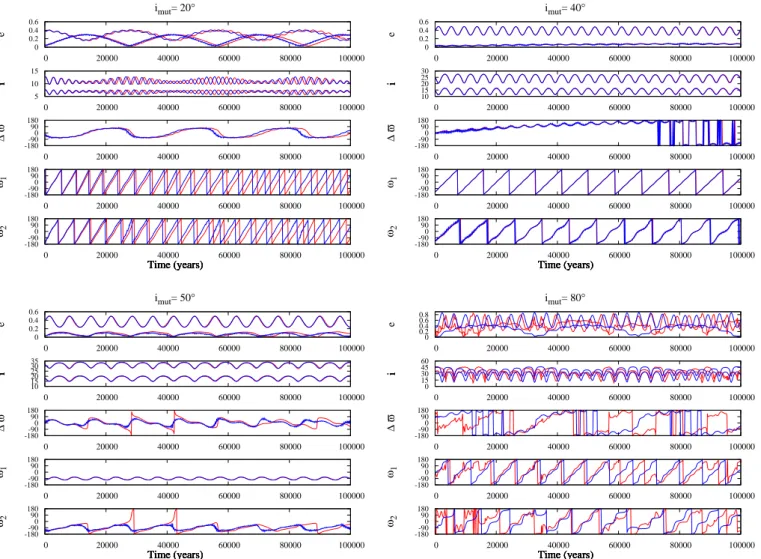
To further illustrate the accuracy of our analytical approach, we show in Fig.1the evolutions of HD 12661 given by the ana-lytical expansion Eq. (5) (red curves) for the mutual inclinations imut = 20◦, 40◦, 50◦, and 80◦ (i is fixed to 50◦), and compare
them to the evolutions obtained by the numerical integration of the three-body problem with the SWIFT package (Levison & Duncan 1994, blue curves). Although the numerical conver-gence observed in Table 2 is not excellent for HD 12661, the agreement of the analytical approach with the numerical integra-tion of the full problem is very good. The dynamical evoluintegra-tions are well reproduced up to high values of the mutual inclina-tion (imut = 20◦, 40◦, 50◦). Only small differences in the
peri-ods are observed and can be attributed to the short-period terms not considered in our secular formulation. For very high values (imut = 80◦), the dynamical evolutions given by the two methods
no longer coincide, but follow the same trend. As will be shown in Sect.4.3, the orbits are generally chaotic at such high mutual inclinations.
4. Results
The question of the 3D secular dynamics of RV-detected plane-tary systems is addressed here in two directions. Firstly, we focus on identifying the inclination values for which a LK-resonant regime is observed in our parametric study. Secondly, the long-term stability of the mutually inclined systems is unveiled by means of a chaos detector.
4.1. Extent of the Lidov-Kozai regions
Regarding the possible 3D configurations of extrasolar sys-tems, we are particularly interested in the LK resonance. This protective mechanism ensures that the system remains stable,
despite large eccentricity and inclination variations. It is char-acterised, in the Laplace-plane reference frame, by the coupled variation of the eccentricity and the inclination of the inner planet, and the libration of the argument of the pericenter of the same planet around ±90◦(Lidov 1962;Kozai 1962).
As a first example, we investigate the dynamics of the HD 12661 extrasolar system. In the left panel of Fig.2, we show, for varying (imut, i) values, the maximal eccentricity of the inner
planet reached during the dynamical evolution of the system, max e1= max
t e1(t), (8)
being e1(t) the eccentricity of the inner planet at time t. Let us
note that this quantity is often used to determine the regularity of planetary orbits, since for low (e < 0.2) and high (e > 0.8) eccentricity values it is generally found to be in good agreement with chaos indicators (see for instanceFunk et al. 2011). On the right panel, we report, for all the considered (imut, i) values, the
libration amplitude of the angle ω1, defined as
libr_ampl (ω1)= max
t ω1(t) − mint ω1(t). (9)
This value will serve as a guide for the detection of the LK-resonant behaviour characterised by the libration of ω1, and thus
by a small value of libr_ampl (ω1).
When following an horizontal line in Fig.2, the mutual incli-nation imut varies while the orbital inclination i, and thus the
planetary masses, are kept fixed. On the other hand, the inclina-tion of the common orbital plane decreases when moving down along a vertical line, while the planetary masses increase accord-ingly. As previously stated, this implies the recomputation of the coefficients Cj,m,nof Eq. (5). Let us recall that all (imut, i) pairs
cannot be considered here since, for fixed i1 = i2 = i values,
Eq. (6) cannot be solved for all the mutual inclinations.
We see that the eccentricity variations of 3D configurations of HD 12661 are small1for low mutual inclinations (blue in the left panel of Fig. 2) and become large for high mutual incli-nations (red). Additionally, the argument of the pericenter ω1
circulates for low imut values (light blue in the right panel of
Fig.2) and librates for high imut values (dark blue). Thus, for
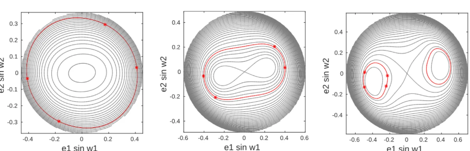
high mutual inclinations, the system is in a LK-resonant state. To visualise the different dynamics, we draw, for a given D2
value, the level curves of the Hamiltonian Eq. (5) in the repre-sentative plane (e1sin ω1, e2sin ω2) where both pericenter
argu-ments are fixed to ±90◦ (seeLibert & Henrard 2007for more
M. Volpi et al.: 3D secular dynamics of RV-detected planetary systems imut= 20° 0 0.2 0.4 0.6 0 20000 40000 60000 80000 100000 e Time (years) 5 10 15 0 20000 40000 60000 80000 100000 Time (years) i -180-90 0 90 180 0 20000 40000 60000 80000 100000 ∆ ϖ Time (years) i -180-90 0 90 180 0 20000 40000 60000 80000 100000 ω1 Time (years) i -180-90 0 90 180 0 20000 40000 60000 80000 100000 ω2 Time (years) i imut= 40° 0 0.2 0.4 0.6 0 20000 40000 60000 80000 100000 e Time (years) 10 15 20 25 30 0 20000 40000 60000 80000 100000 Time (years) i -180-90 0 90 180 0 20000 40000 60000 80000 100000 ∆ ϖ Time (years) i -180-90 0 90 180 0 20000 40000 60000 80000 100000 ω1 Time (years) i -180-90 0 90 180 0 20000 40000 60000 80000 100000 ω2 Time (years) i imut= 50° 0 0.2 0.4 0.6 0 20000 40000 60000 80000 100000 e Time (years) 10 15 20 25 30 35 0 20000 40000 60000 80000 100000 Time (years) i -180-90 0 90 180 0 20000 40000 60000 80000 100000 ∆ ϖ Time (years) i -180-90 0 90 180 0 20000 40000 60000 80000 100000 ω1 Time (years) i -180-90 0 90 180 0 20000 40000 60000 80000 100000 ω2 Time (years) i imut= 80° 0 0.2 0.4 0.6 0.8 0 20000 40000 60000 80000 100000 e Time (years) 0 15 30 45 60 0 20000 40000 60000 80000 100000 Time (years) i -180-90 0 90 180 0 20000 40000 60000 80000 100000 ∆ ϖ Time (years) i -180-90 0 90 180 0 20000 40000 60000 80000 100000 ω1 Time (years) i -180-90 0 90 180 0 20000 40000 60000 80000 100000 ω2 Time (years) i
Fig. 1.Dynamical evolutions of HD 12661 system given by the analytical expansion (in red) and by n-body simulations (in blue), for imut= 20◦
(top left), 40◦
(top right), 50◦
(bottom left), and 80◦
(bottom right). The inclination of the orbital plane is fixed to i= 50◦
.
HD12661: Max e
10
10 20 30 40 50 60 70 80
i
mut(deg)
0
15
30
45
60
75
90
i (deg)
0
0.2
0.4
0.6
0.8
1
HD12661:
ω
1libration amplitude
0
10 20 30 40 50 60 70 80
i
mut(deg)
0
15
30
45
60
75
90
i (deg)
0
50
100
150
200
250
300
350
Fig. 2. Long-term evolution of HD 12661 system when varying the mutual inclination imut (x-axis) and the inclination of the orbital plane i
(y-axis), both expressed in degrees. Left panel: maximal eccentricity of the inner planet, as defined by Eq. (8). Right panel: libration amplitude of
the argument of the pericenter ω1(in degrees), as defined by Eq. (9). The three highlighted points are related to the representative planes shown in
Fig.3.
details on the representative plane). This plane is neither a phase portrait nor a surface of section, since the problem is four dimen-sional. However, nearly all the orbits will cross the representa-tive plane at several points of intersection on the same energy curve. Figure3shows the representative planes of HD 12661 for
imut = 20◦ (i.e. D2 = 0.35, left panel), 40◦ (i.e. D2 = 0.67,
middle panel), and 50◦(i.e. D2 = 0.90, right panel), the
inclina-tion of the orbital plane being fixed to 50◦. These three system
configurations are also indicated with white crosses in Fig.2and their dynamical evolutions are those presented in Fig.1.
e1 sin w1 -0.4 -0.2 0 0.2 0.4 e2 sin w2 -0.3 -0.2 -0.1 0 0.1 0.2 0.3 e1 sin w1 -0.6 -0.4 -0.2 0 0.2 0.4 0.6 e2 sin w2 -0.4 -0.2 0 0.2 0.4 e1 sin w1 -0.6 -0.4 -0.2 0 0.2 0.4 0.6 e2 sin w2 -0.4 -0.2 0 0.2 0.4
Fig. 3.Representative plane for HD 12661 system, having fixed the inclination of the orbital plane to i= 50◦
, for imut= 20◦(left panel), imut= 40◦
(middle panel), and imut = 50◦(right panel). The level curve of Hamiltonian relative to the orbital parameters of HD 12661 is highlighted in red.
The crosses indicate the intersections of the orbit with the representative plane.
HD11506: Max e
10
10 20 30 40 50 60 70 80
i
mut(deg)
0
15
30
45
60
75
90
i (deg)
0
0.2
0.4
0.6
0.8
1
HD11506:
ω
1libration amplitude
0
10 20 30 40 50 60 70 80
i
mut(deg)
0
15
30
45
60
75
90
i (deg)
0
50
100
150
200
250
300
350
Fig. 4.Same as Fig.2for HD 11506 system.
For low values of imut, circular orbits (e1 = e2 = 0)
con-stitute a point of stable equilibrium (left panel of Fig. 3). As we increase the mutual inclination (central and right panels of Fig.3), the central equilibrium becomes unstable and bifurcates into the two stable LK equilibria. The red crosses represent the intersections of the evolution of the mutually inclined HD 12661 system with the representative plane. For low mutual inclina-tions, the crosses are located on both sides of the representa-tive plane, so the argument of the inner pericenter circulates. For imut = 50◦(right panel of Fig.3), the crosses are inside the LK
island in the left side of the representative plane, associated with the libration of ω1around 270◦(as can also be observed in the
bottom left dynamical evolution shown in Fig.1). We see that the corresponding white cross on the right side of Fig.2is likewise located inside the dark blue region of the LK resonance.
The critical value of the mutual inclination, which corre-sponds to the change of stability of the central equilibrium, depends on the mass and semi-major axis ratios (see e.g. Libert & Henrard 2007) and is typically around 40◦−45◦ for
mass ratios between 0.5 and 2. For increasing mutual inclina-tions, the stable LK equilibria reach higher inner eccentricity values and the orbit of the considered system possibly crosses the representative plane inside a LK island. Therefore, the dark blue LK region in Fig.2starts around 40◦−55◦, the exact value
for the change of dynamics depending on the inclination of the orbital plane since the expansion (Eq.5) depends on the inclina-tion i via the planetary mass.
Let us note that, even if the numerical convergence of the analytical expansion of the HD 12661 system is not excellent (see Table2), the LK-resonant region perfectly matches the one obtained with n-body simulations additionally performed for validation, except at very high mutual inclinations (imut ≥ 70◦).
Indeed, for the HD 12661 and HD 74156 systems, a destabilisa-tion of the orbits is observed at very high mutual inclinadestabilisa-tions and slightly reduces the stable LK region.
A second example is shown in Fig.4for the HD 11506 sys-tem. The LK region is now located at smaller mutual inclina-tions, making visible the right border of the LK region. For each i value, the interval of mutual inclinations associated with the libration of the angle ω1 begins at ∼40◦, whereas its amplitude
depends on i. No spatial configuration of HD 11506 can be found in a LK-resonant state for a mutual inclination higher than 65◦.
Let us note that some additional dark blue points can be observed for low values of the inclinations of the orbital plane i. These systems are close to the separatrix of the LK resonance and will be destabilised on a longer timescale, as will be shown in the next section.
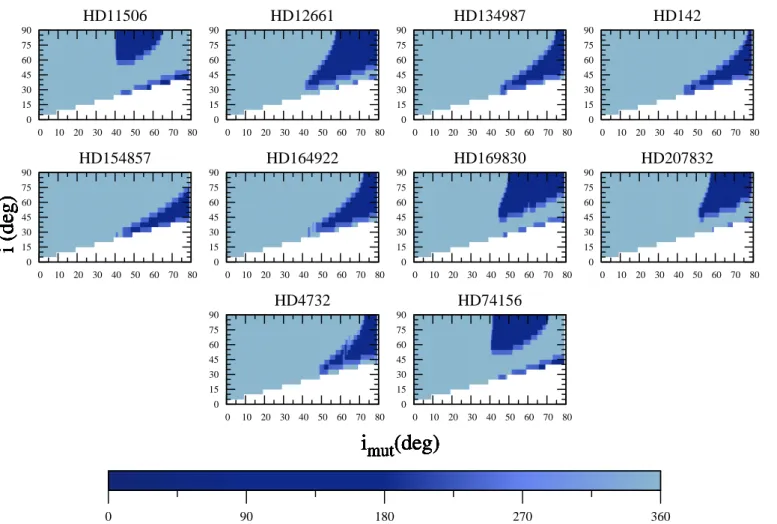
In Fig. 5 we display the libration amplitude of the argu-ment of the pericenter of the inner planet for the ten systems considered here. All the graphs do show a LK region. In other words, all the selected RV-detected systems, when considered with a significant mutual inclination, have physical and orbital parameters compatible with a LK-resonant state. Table3 sum-marises information on the extent of the LK region for each
M. Volpi et al.: 3D secular dynamics of RV-detected planetary systems
HD11506
i
mut
(deg)
i (deg)
0 10 20 30 40 50 60 70 80 0 15 30 45 60 75 90HD12661
i
mut
(deg)
i (deg)
0 10 20 30 40 50 60 70 80 0 15 30 45 60 75 90HD134987
i
mut
(deg)
i (deg)
0 10 20 30 40 50 60 70 80 0 15 30 45 60 75 90HD142
i
mut
(deg)
i (deg)
0 10 20 30 40 50 60 70 80 0 15 30 45 60 75 90HD154857
i
mut
(deg)
i (deg)
0 10 20 30 40 50 60 70 80 0 15 30 45 60 75 90HD164922
i
mut
(deg)
i (deg)
0 10 20 30 40 50 60 70 80 0 15 30 45 60 75 90HD169830
i
mut
(deg)
i (deg)
0 10 20 30 40 50 60 70 80 0 15 30 45 60 75 90HD207832
i
mut
(deg)
i (deg)
0 10 20 30 40 50 60 70 80 0 15 30 45 60 75 90HD4732
i
mut
(deg)
i (deg)
0 10 20 30 40 50 60 70 80 0 15 30 45 60 75 90HD74156
i
mut
(deg)
i (deg)
0 10 20 30 40 50 60 70 80 0 15 30 45 60 75 90i
mut
(deg)
i (deg)
0 90 180 270 360Fig. 5.Libration amplitude of ω1for the ten systems considered here, when varying the mutual inclination imut(x-axis) and the inclination of the
orbital plane i (y-axis).
Table 3. Extent of the LK region for the ten systems.
System min imut min i LK chaos
(◦) (◦) (%) (%) HD 11506 41 30 15 39 HD 12661 43 30 24 49 HD 134987 46 30 13 – HD 142 44 30 11 2 HD 154857 41 30 10 2 HD 164922 43 30 23 – HD 169830 45 25 23 19 HD 207832 50 35 17 20 HD 4732 49 35 12 15 HD 74156 41 30 20 2
Notes. For each system, we indicate the minimum imut(second column)
and i (third column) values of the LK region where libration of ω1 is
observed in Fig.5, the percentage of initial conditions for which a
LK-resonant state is observed (fourth column), and the percentage of initial conditions classified as chaotic by the chaos indicator (fifth column).
system. The second and third columns display the minimum val-ues of the mutual inclination imut (with an accuracy of 1◦) and
the orbital inclination i, respectively, for which a libration of the argument of the pericenter ω1 is observed. The percentage of
initial conditions inside the (dark blue) LK region is given in the fourth column. The last column reports the percentage of
chaos in the whole set of initial conditions and will be discussed in Sect.4.3.
4.2. Sensitivity to observational uncertainties
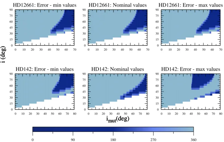
So far, we have considered the nominal values of the orbital parameters given by the observations. However, due to the limi-tations of the detection techniques, observational data come with relevant uncertainties, and to explore the influence of such uncer-tainties on the previous results is relevant. As typical examples, we show in Fig.6the extent of the LK region for the HD 12661 and HD 142 systems, when considering extremal orbital param-eters within the confidence regions given by the observations, instead of the best-fit parameter values. The errors on each orbital parameter are listed in Table1 for both planetary sys-tems. Two extremal cases are examined in the following, where the minimal/maximal values are adopted for all the parameters simultaneously.
In the case of the HD 12661 system, the location and extent of the LK region are very similar when adopting the minimal values (top left panel of Fig.6), the nominal values (top mid-dle), and the maximal values (top right) of the orbital parameters. Concerning HD 142, the situation is quite different. We observe, in the bottom panels of Fig.6, a significant variation of the LK region in its extent and shape, probably due to the greater size of the observational errors on the different orbital elements.
As a result, the location and extent of the LK resonance regions are sensitive to observational uncertainties in the orbital
HD12661: Error - min values
i
mut
(deg)
i (deg)
0 10 20 30 40 50 60 70 0 15 30 45 60 75 90HD12661: Nominal values
i
mut
(deg)
i (deg)
0 10 20 30 40 50 60 70 0 15 30 45 60 75 90HD12661: Error - max values
i
mut
(deg)
i (deg)
0 10 20 30 40 50 60 70 0 15 30 45 60 75 90HD142: Error - min values
i
mut
(deg)
i (deg)
0 10 20 30 40 50 60 70 80 0 15 30 45 60 75 90HD142: Nominal values
i
mut
(deg)
i (deg)
0 10 20 30 40 50 60 70 80 0 15 30 45 60 75 90HD142: Error - max values
i
mut
(deg)
i (deg)
0 10 20 30 40 50 60 70 80 0 15 30 45 60 75 90i
mut
(deg)
i (deg)
0 90 180 270 360Fig. 6.Libration amplitude of ω1, as in Fig.5, for the HD 12661 (top) and HD 142 (bottom) systems, when considering the minimal values (left),
the nominal values (middle), and the maximal values (right) of the orbital parameters.
elements, especially when they are significant, and this should be taken into account in detailed studies of the selected systems. Nevertheless, we stress that, when considering extremal values within the confidence regions, the dynamics remains qualita-tively the same, with the existence of stable LK islands at high mutual inclinations for both systems.
4.3. Stability of planetary systems
In this section, we aim to determine if the LK-resonant state of a 3D planetary system is essential to ensure its long-term stability. To do so, we have used the Mean Exponential Growth factor of Nearby Orbits (MEGNO) chaos indicator, briefly described in the following (for an extensive discussion on the properties of the MEGNO, seeCincotta & Simo 2000;Maffione et al. 2011).
Let H(p, q) with p, q ∈ RN be an autonomous Hamiltonian
of N degrees of freedom. The Hamiltonian vector field can be expressed as ˙x= J∇xH x, (10) where x = p q ! ∈ R2N and J ="0N − 1N 1N 0N # , being 1N and
0N the unitary and null N × N matrices, respectively. In order
to apply the MEGNO chaos indicator, we need to compute the evolution of deviation vectors δ(t). These vectors satisfy the vari-ational equations
˙
δ(t) = J∇2
xHδ(t), (11)
being ∇2xH the Hessian matrix of the Hamiltonian. As in
Cincotta & Simo (2000), the Mean Exponential Growth
Factor is defined as Y(t)=2 t Z t 0 ˙ δ(s) δ(s)ds, (12)
where δ(s) is the Euclidean norm of δ(s). We consider here the mean MEGNO, that is, the time-averaged MEGNO,
¯ Y(t)=1 t Z t 0 Y(s) ds. (13)
The limit for t → ∞ provides a good characterisation of the orbits. The MEGNO chaos indicator is particularly convenient since we have:
– limt→∞Y¯(t)= 0 for stable periodic orbits,
– limt→∞Y¯(t)= 2 for quasi-periodic orbits and for orbits close
to stable periodic ones,
– for irregular orbits, ¯Y(t) diverges with time.
For each set of initial conditions we choose the initial deviation vector δ(0) as a random unitary vector. We then study its evolu-tion along the orbit and compute the corresponding evoluevolu-tion of the mean MEGNO. Two main factors have motivated the choice of this chaos indicator. First, it requires the study of the evolu-tion of only one deviaevolu-tion vector, saving valuable computaevolu-tional time. Second, it returns an absolute value, as it classifies each orbit independently.
As previously noted, the LK-resonant state is surrounded by a chaotic zone associated with the bifurcation of the central equi-librium at null eccentricities. Therefore, a chaos indicator can be useful to highlight the extent of the chaotic zone and identify with precision the (imut, i) values ensuring the regularity of the
orbits for a long time.
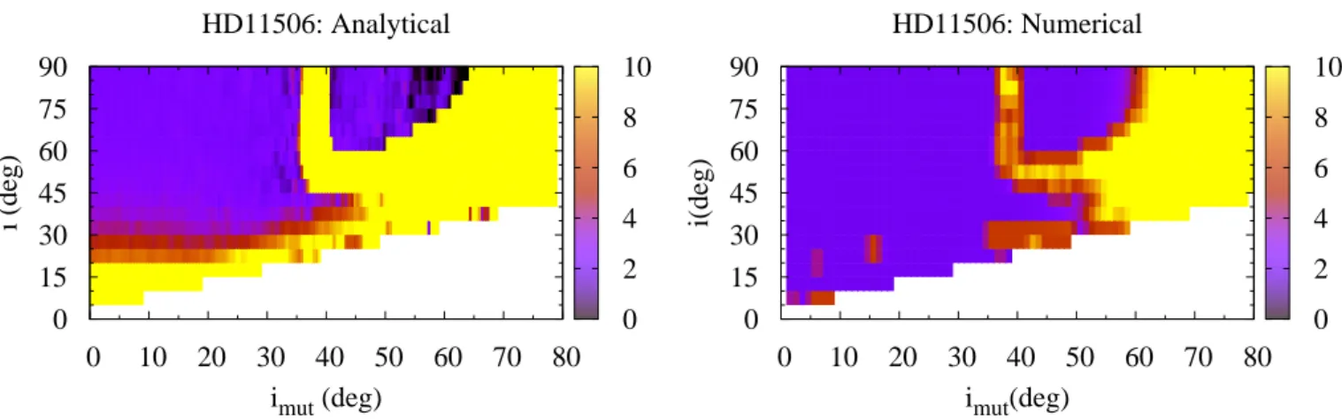
On the left panel of Fig.7, we show the values of the mean MEGNO for HD 11506 computed with our analytical approach.
M. Volpi et al.: 3D secular dynamics of RV-detected planetary systems
HD11506: Analytical
0
10 20 30 40 50 60 70 80
i
mut(deg)
0
15
30
45
60
75
90
i (deg)
0
2
4
6
8
10
HD11506: Numerical
0
10 20 30 40 50 60 70 80
i
mut(deg)
0
15
30
45
60
75
90
i(deg)
0
2
4
6
8
10
Fig. 7.Mean MEGNO values for the HD 11506 system given by our analytical approach (left panel) and n-body simulations (right panel).
HD11506
i
mut
(deg)
i (deg)
0 10 20 30 40 50 60 70 80 0 15 30 45 60 75 90HD12661
i
mut
(deg)
i (deg)
0 10 20 30 40 50 60 70 80 0 15 30 45 60 75 90HD134987
i
mut
(deg)
i (deg)
0 10 20 30 40 50 60 70 80 0 15 30 45 60 75 90HD142
i
mut
(deg)
i (deg)
0 10 20 30 40 50 60 70 80 0 15 30 45 60 75 90HD154857
i
mut
(deg)
i (deg)
0 10 20 30 40 50 60 70 80 0 15 30 45 60 75 90HD164922
i
mut
(deg)
i (deg)
0 10 20 30 40 50 60 70 80 0 15 30 45 60 75 90HD169830
i
mut
(deg)
i (deg)
0 10 20 30 40 50 60 70 80 0 15 30 45 60 75 90HD207832
i
mut
(deg)
i (deg)
0 10 20 30 40 50 60 70 80 0 15 30 45 60 75 90HD4732
i
mut
(deg)
i (deg)
0 10 20 30 40 50 60 70 80 0 15 30 45 60 75 90HD74156
i
mut
(deg)
i (deg)
0 10 20 30 40 50 60 70 80 0 15 30 45 60 75 90i
mut
(deg)
i (deg)
0 90 180 270 360Fig. 8.Same as Fig.5, where the initial system parameters leading to chaotic motion (defined by the mean MEGNO value greater than 8) are coloured in white (above the black curve).
We can appreciate how the region at high inclinations charac-terised as regular by the mean MEGNO (purple) clearly super-imposes with the LK-resonant region identified in Fig 4. The surrounding chaotic region displayed in yellow extends up to high mutual inclinations, showing that highly mutually inclined configurations of the HD 11506 system can only be expected in a LK-resonant state. Regarding low mutual inclinations, nearly all spatial configurations present regular motion up to a mutual inclination of ∼35◦, where the LK resonance comes into play.
A comparison with n-body simulations (short-period effects included) is given in the right panel of Fig.7, where numerical
integrations have been carried out with SWIFT (for every 1◦ instead of 0.5◦to reduce the computational cost). The two panels
look very similar, showing that our secular approach is reliable for systems that are far from a mean-motion resonance.
Similar observations can be made for the ten extrasolar sys-tems considered here. In Fig.8, the chaotic region associated to a mean MEGNO value greater than eight with our analyt-ical approach, is indicated in white on the plot showing the libration amplitude of ω1 (Fig.5). Also, more information on
the extent of the chaotic zone for each system can be found in the last column of Table 3. The chaotic region around the
stable LK islands is broad for half of the systems (HD 11506, HD 12661, HD 169830, HD 207832, and HD 4732), moderate for the HD 142, HD 15487, and HD 74156 systems, and not sig-nificant for the HD 134987 and HD 164922 systems, given the integration timescale and the grid of initial conditions consid-ered. For the first category of systems, long-term regular evolu-tions of the orbits are only possible for low mutual inclinaevolu-tions and, for higher mutual inclinations, in the LK region, while in the two other cases regular evolutions are also observed at high mutual inclinations outside the LK regions.
5. Conclusions
In this work, we studied the possibility for ten RV-detected exo-planetary systems to be in a 3D configuration. Using a secu-lar Hamiltonian approximation (expansion in eccentricities and inclinations), we studied the secular dynamics of possible 3D planetary configurations of the systems. In particular, we deter-mined ranges of orbital and mutual inclinations for which the system is in a LK-resonant state. Our results were compared with n-body simulations, showing the accuracy of the analytical approach up to very high inclinations (∼70◦−80◦). We showed
that all the systems considered here might be in a LK-resonant state for a sufficiently mutually inclined orbit. By means of the MEGNO chaos indicator, we revealed the extent of the chaotic zone surrounding the stability islands of the LK resonance. Long-term regular evolutions of the orbits are possible (i) at low mutual inclinations and (ii) at high mutual inclinations, preferen-tially in the LK region, due to the significant extent of the chaotic zone in many systems.
It should be stressed that the present work excludes systems whose inner planet is close to the star. For those systems, rela-tivistic effects have to be considered and we leave for future work how their inclusion will influence the extent of the LK region. Acknowledgements. The authors thank the anonymous referee for her or his critical review of the first version of the manuscript and useful suggestions. M.V. acknowledges financial support from the FRIA fellowship (F.R.S.-FNRS). The
work of A.R. is supported by a F.R.S.-FNRS research fellowship. Computational resources have been provided by the PTCI (Consortium des Équipements de Cal-cul Intensif CECI), funded by the FNRS-FRFC, the Walloon Region, and the University of Namur (Conventions No. 2.5020.11, GEQ U.G006.15, 1610468 et RW/GEQ2016).
References
Arnol’d, V. I. 1963,Russ. Math. Surv., 18, 9
Cincotta, P. M., & Simo, C. 2000,A&AS, 147, 205
Dawson, R. I., & Chiang, E. 2014,Science, 346, 212
Deitrick, R., Barnes, R., McArthur, B., et al. 2015,ApJ, 798, 46
Feng, Y. K., Wright, J. T., Nelson, B., et al. 2015,ApJ, 800, 22
Fulton, B. J., Howard, A. W., Weiss, L. M., et al. 2016,ApJ, 830, 46
Funk, B., Libert, A.-S., Süli, Á., & Pilat-Lohinger, E. 2011, A&A, 526, A98
Haghighipour, N., Butler, R. P., Rivera, E. J., Henry, G. W., & Vogt, S. S. 2012,
ApJ, 756, 91
Jones, H. R. A., Butler, R. P., Tinney, C. G., et al. 2010,MNRAS, 403, 1703
Kolmogorov, A. N. 1954,Dokl. Akad. Nauk SSSR, 98, 527
Kozai, Y. 1962,AJ, 67, 591
Levison, H. F., & Duncan, M. J. 1994,Icarus, 108, 18
Libert, A.-S., & Henrard, J. 2005,Celest. Mech. Dyn. Astron., 93, 187
Libert, A.-S., & Henrard, J. 2007,Icarus, 191, 469
Libert, A.-S., & Henrard, J. 2008,Celest. Mech. Dyn. Astron., 100, 209
Libert, A.-S., & Sansottera, M. 2013,Celest. Mech. Dyn. Astron., 117, 149
Libert, A.-S., & Tsiganis, K. 2009,A&A, 493, 677
Lidov, M. L. 1962,Planet. Space Sci., 9, 719
Maffione, N. P., Giordano, C. M., & Cincotta, P. M. 2011,Int. J. Non-Linear Mech., 46, 23
Mayor, M., Udry, S., Naef, D., et al. 2004,A&A, 415, 391
Michtchenko, T. A., Ferraz-Mello, S., & Beaugé, C. 2006,Icarus, 181, 555
Moser, J. 1962,Matematika, 6, 51
Poincaré, H. 1893,Les méthodes nouvelles de la mécanique céleste: Méthodes de MM. Newcomb, Glydén, Lindstedt et Bohlin(Gauthier-Villars et fils) Robutel, P. 1995,Celest. Mech. Dyn. Astron., 62, 219
Sato, B., Omiya, M., Wittenmyer, R. A., et al. 2013,ApJ, 762, 9
Tuomi, M., & Kotiranta, S. 2009,A&A, 496, L13
Veras, D., & Ford, E. B. 2010,ApJ, 715, 803
Volpi, M., Locatelli, U., & Sansottera, M. 2018,Celest. Mech. Dyn. Astron., 130, 36
Wittenmyer, R. A., Horner, J., Tuomi, M., et al. 2012,ApJ, 753, 169
Wittenmyer, R. A., Horner, J., Tinney, C. G., et al. 2014,ApJ, 783, 103