HAL Id: tel-02495038
https://tel.archives-ouvertes.fr/tel-02495038v2
Submitted on 23 Mar 2020
HAL is a multi-disciplinary open access
archive for the deposit and dissemination of sci-entific research documents, whether they are pub-lished or not. The documents may come from teaching and research institutions in France or abroad, or from public or private research centers.
L’archive ouverte pluridisciplinaire HAL, est destinée au dépôt et à la diffusion de documents scientifiques de niveau recherche, publiés ou non, émanant des établissements d’enseignement et de recherche français ou étrangers, des laboratoires publics ou privés.
applications to image segmentation
Deise Santana Maia
To cite this version:
Deise Santana Maia. A study of hierarchical watersheds on graphs with applications to image seg-mentation. Image Processing [eess.IV]. Université Paris-Est, 2019. English. �NNT : 2019PESC2069�. �tel-02495038v2�
UNIVERSITE PARIS-EST
ECOLE DOCTORALE MSTIC
Discipline : Informatique
Deise Santana Maia
A study of hierarchical watersheds on graphs with
applications to image segmentation
Soutenue publiquement à ESIEE Paris le 10/12/2019 devant le jury composé de :
Jesus ANGULO MINES ParisTech Raporteur
Gunilla BORGEFORS Uppsala University Rapportrice
Jean COUSTY Université Paris-Est Co-encadrant
Mauro DALLA MURA Institut Polytechnique de Grenoble Examinateur
Bertrand KERAUTRET Université Lumière Lyon 2 Examinateur et Président
Laurent NAJMAN Université Paris-Est Directeur de thèse
Acknowledgments
I am grateful for all the professors and mentors that guided my education during my years as a bachelor, master and PhD student. Thank you Roque Trindade and Alexsan-dra Oliveira for inspiring me to follow an academic career after proposing my first project on image processing and mathematical morphology. Thank you Arnaldo Araujo for ac-cepting being my master advisor and for helping me to pursue my studies as an exchange student at Université Paris-Est. Finally, my special thanks go to my PhD advisors Jean Cousty, Laurent Najman and Benjamin Perret. I feel very lucky and grateful to have collaborated with you. You have been helpful and supportive all way through my PhD studies, always ready to revise my writing, to discuss new ideas, to help me improving my speech skills... Most importantly, you helped me to be more rigorous and confident on my work.
Thank you all the members of the jury (Jesus Angulo, Gunilla Borgefors, Mauro Dalla Mura and Bertrand Keuratret) for accepting to revise my manuscript and to take part in my PhD defense.
To all my colleagues and friends who were present at some point during those years, thank you for sharing nice moments and the ups and downs of being a PhD student. Thank you Bruno Jartoux, Clara Jaquet, Daniel Antunes, Diane Genest, Duc Nguyen, Edward Cayllahua, Elias Barbudo, Evgeny Chzhen, Gisela Domej, Kacper Pluta, Karla Otiniano, Ketan Bacchuwar, Lama Tarsissi, Monika Csikos, Rosembergue Rodrigues, Stéphane Breuils, Thanh Xuan Nguyen, Tina Malalanirainy and Yukiko Kenmochi.
To my dear Thuy, thank you for your love, patience and for always being there for me. Thank you also for our interesting discussions on watersheds, which inspired me to investigate new ideas on this topic.
Last but not least, I thank my family for their unconditional love and all the efforts they made so I could be here today. I thank my father Jaime, for being an amazing, caring and loving person, who did everything that he could to give me a good education. He always hoped that everything would be better one day, and, thank to his hard work, it did get better! I thank my mother Emiliana for leading by example that there is always something else that you could learn and that it is never too late to do that. Thank
Denise for your positive attitude in life and for always being ready to help people around you. Thank you Daniela (in memoriam) for always taking care of me. I dedicate this thesis to you.
Abstract
The wide literature on graph theory invites numerous problems to be modeled in the framework of graphs. In particular, clustering and segmentation algorithms designed in this framework can be applied to solve problems in various domains, including image processing, which is the main field of application investigated in this thesis. In this work, we focus on a semi-supervised segmentation tool widely studied in mathematical morphology and used in image analysis applications, namely the watershed transform. We explore the notion of a hierarchical watershed, which is a multiscale extension of the notion of watershed allowing to describe an image or, more generally, a dataset with partitions at several detail levels. The main contributions of this study are the following:
• Recognition of hierarchical watersheds: we propose a characterization of hierarchical watersheds which leads to an efficient algorithm to determine if a hierarchy is a hierarchical watershed of a given edge-weighted graph.
• Watersheding operator: we introduce the watersheding operator, which, given an edge-weighted graph, maps any hierarchy of partitions into a hierarchical watershed of this edge-weighted graph. We show that this operator is idempotent and its fixed points are the hierarchical watersheds. We also propose an efficient algorithm to compute the result of this operator.
• Probability of hierarchical watersheds: we propose and study a notion of probability of hierarchical watersheds, and we design an algorithm to compute the probability of a hierarchical watershed. Furthermore, we present algorithms to compute the hierarchical watersheds of maximal and minimal probabilities of a given weighted graph.
• Combination of hierarchies: we investigate a family of operators to combine hier-archies of partitions and study the properties of these operators when applied to hierarchical watersheds. In particular, we prove that, under certain conditions, the family of hierarchical watersheds is closed for the combination operator.
In conclusion, this thesis reviews existing and introduces new properties and algo-rithms related to hierarchical watersheds, showing the theoretical richness of this frame-work and providing insightful view for its applications in image analysis and computer vision and, more generally, for data processing and machine learning.
Résumé
La littérature abondante sur la théorie des graphes invite de nombreux problèmes à être modélisés dans ce cadre. En particulier, les algorithmes de regroupement et de segmen-tation conçus dans ce cadre peuvent être utilisés pour résoudre des problèmes dans de nombreux domaines tels que l’analyse d’image qui est le principal domaine d’application de cette thèse. Dans ce travail, nous nous concentrons sur un outil de segmentation semi-supervisé largement étudié dans la morphologie mathematique et appliqué à l’analyse d’image, notamment les Ligne de Partage des Eaux (LPE). Nous étudions la notion de hiérarchie de LPE, qui est une extension multi-échelle de la notion de LPE permettant de décrire une image ou, plus généralement, un ensemble de donnés par des partitions à plusieurs niveaux de détail. Les contributions principales de cette étude sont les suiv-antes :
• Reconnaissance de hiérarchies de LPE : nous proposons une caractérisation des hiérarchies de LPE qui mène à un algorithme efficace pour déterminer si une hiérar-chie est une hiérarhiérar-chie de LPE d’un graphe donné.
• Opérateur watersheding : nous présentons l’opérateur watersheding, qui, étant donné un graphe pondéré, associe n’importe quelle hiérarchie à une hiérarchie de LPE de ce graphe. Nous montrons que cet opérateur est idempotent et que ses points fixes sont les hiérarchies de LPE. Nous proposons également un algorithme efficace pour calculer le résultat de cet opérateur.
• Probabilité de hiérarchies de LPE : nous proposons et étudions une notion de probabilité d’une hiérarchie de LPE, et nous concevons un algorithme pour calculer la probabilité d’une hiérarchie de LPE. De plus, nous présentons des algorithmes pour calculer des hiérarchies de LPE de probabilité minimale et maximale pour un graphe pondéré donné.
• Combinaison de hiérarchies : nous étudions une famille d’opérateurs pour com-biner des hiérarchies de partitions et nous étudions les propriétés de ces opérateurs lorsqu’ils sont appliqués à les hiérarchies de LPE. En particulier, nous prouvons
• Évaluation de hiérarchies : nous proposons un cadre d’évaluation de hiérarchies, qui est également utilisé pour évaluer les hiérarchies de LPE et les combinaisons des hiérarchies.
En conclusion, cette thèse révise des propriétés existantes et des nouvelles propriétés liées aux hiérarchies de LPE, montrant la richesse théorique de ce cadre et fournissant une vue d’ensemble des ses applications dans l’analyse d’image et dans la vision par ordinateur et, plus généralement, dans le traitement de donnés et dans l’apprentissage automatique.
Contents
Chapter 1 – Introduction 13
Chapter 2 – Hierarchies and Graphs 21
2.1 Graphs . . . 21
2.2 Hierarchies of partitions . . . 22
2.3 Quasi-flat zones hierarchies . . . 28
2.4 Contour saliency maps . . . 30
2.5 Binary partition trees . . . 33
2.6 Hierarchical watersheds . . . 36
2.7 Attribute based hierarchies . . . 48
Chapter 3 – Characterization and recognition of hierarchical wa-tersheds 59 3.1 Introduction . . . 59
3.2 Characterization of hierarchical watersheds . . . 62
3.3 Algorithm to recognize hierarchical watersheds . . . 66
3.4 Flattened hierarchical watersheds . . . 67
3.5 Conclusion . . . 70
Chapter 4 – Watersheding hierarchies 73 4.1 Introduction . . . 73
4.2 Watersheding operator . . . 76
4.3 Watersheding operator algorithm . . . 82
4.4 Illustrations of applications in image analysis . . . 83
4.5 Conclusion . . . 85
Chapter 5 – Probability of hierarchical watersheds 91 5.1 Introduction . . . 91
5.2 Studying probabilities of hierarchical watersheds . . . 94
5.3 Algorithm to compute the probability of a hierarchical watershed . . . . 96
5.4 Most and least probable hierarchical watersheds . . . 97 5.5 Algorithms to compute a most and a least probable hierarchical watershed 101
Chapter 6 – Evaluation framework of hierarchies of segmentations 107
6.1 Introduction . . . 107
6.2 Cut of a hierarchy . . . 108
6.3 Number of parent nodes . . . 109
6.4 Baseline: precision-recall for boundaries . . . 110
6.5 Proposed evaluation methodology . . . 111
6.6 Experiments . . . 115
6.7 Conclusion . . . 121
Chapter 7 – Combination of hierarchies 123 7.1 Introduction . . . 123
7.2 General combination framework . . . 127
7.3 Normalization of saliency maps . . . 130
7.4 Visual inspection of combinations of hierarchies . . . 131
7.5 Quantitative assessment of combinations of hierarchical watersheds . . . 142
7.6 Properties of combinations of hierarchical watersheds . . . 149
7.7 Recognition of hierarchical watersheds applied to combinations of hierarchies153 7.8 Watersheding of combinations of hierarchical watersheds . . . 155
7.9 Conclusion . . . 157
Chapter 8 – Conclusion 159
References 163
Appendix: proofs of theorems and properties I 8.1 Proofs of theorem and properties of Chapter 3 . . . I 8.2 Proofs of theorem and properties of Chapter 4 . . . XXVII 8.3 Proofs of theorem and properties of Chapter 5 . . . XLIV 8.4 Proofs of theorem and properties of Chapter 7 . . . L
List of figures
1.1 Graph representation of the seven bridges of Königsberg . . . 14
2.1 The representation of a graph and of a hierarchy . . . 22
2.2 A gray-scale and a color image. . . 24
2.3 An image partition . . . 24
2.4 A saliency map . . . 32
2.5 A weighted graph and its binary partition hierarchy . . . 36
2.6 A weighted graph and one of its hierarchical watersheds . . . 40
2.7 Marked-based segmentation with min-cuts . . . 42
2.8 Marked-based segmentation with average-cuts . . . 43
2.9 Marked-based segmentation with shortest path forests . . . 44
2.10 Watershed segmentation . . . 45
2.11 Hierarchical watersheds based on increasing attributes . . . 54
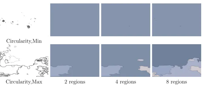
2.12 Non-increasing attributes: circularity, rectangularity and perimeter . . . 55
2.13 Hierarchical watersheds based on regularized circularity . . . 56
2.14 Hierarchies based on non-increasing attributes . . . 57
3.1 Illustration of the notion of building edge and suppremum descendant map 63 3.2 Illustration of the notion of one-side increasing map . . . 65
3.3 Toy example of the algorithm to recognize hierarchical watersheds . . . . 69
4.1 A hierarchical watershed based on regularized circularity and the result of the watersheding operator . . . 75
4.2 Illustration of the notion of extinction map . . . 77
4.3 Illustration of the notions of dominant region and approximated extinction map . . . 80
4.4 Illustrations of the notions of estimated sequence of minima and water-sheding operator . . . 81
4.5 Watersheding of hierarchies based on non-increasing attributes . . . 86
4.6 Watersheding of hierarchies based on non-increasing attributes . . . 87 7
5.1 Example of watershed segmentations obtained from multiple orderings of
the minima . . . 92
5.2 A graph and its binary partition hierarchy . . . 95
5.3 Illustration of the notion of maximal region . . . 95
5.4 Probabilities of the hierarchical watersheds of a given graph . . . 100
5.5 Least and most probable hierarchical watersheds of two gradients . . . . 106
6.1 Cut of a hierarchy . . . 109
6.2 Number of parent nodes . . . 109
6.3 Illustration of under- and over-segmentation for hierarchies . . . 113
6.4 Markers obtained by erosion and skeletonization . . . 115
6.5 Influence of the gradient on dynamics and area based hierarchical watersheds117 6.6 Influence of the area filter on quasi-flat zone hierarchies . . . 119
6.7 Influence of area filtering on dynamics based hierarchical watershed . . . 119
6.8 Best achieved results for each hierarchy and a high quality hierarchical segmentation methods . . . 120
7.1 Combination of two hierarchical watersheds by average . . . 125
7.2 Scheme of our method to combine hierarchical watersheds . . . 128
7.3 Illustration of combinations by infimum and concatenation . . . 129
7.4 Intuitive idea of the concatenation of hierarchies . . . 129
7.5 Normalization of saliency maps . . . 131
7.6 Image gradients: Lab and SED . . . 132
7.7 Combination by infimum using Lab gradient . . . 133
7.8 Combination by infimum using SED gradient . . . 134
7.9 Combination by supremum using Lab gradient . . . 135
7.10 Combination by supremum using SED gradient . . . 136
7.11 Combination by average using Lab gradient . . . 137
7.12 Combination by average using SED gradient . . . 138
7.13 Combination by concatenation using SED gradient . . . 139
7.14 Combination of area and circularity based hierarchies . . . 141
7.15 Combination of area and circularity based hierarchies . . . 142
7.16 Combination of dynamics and perimeter based hierarchies . . . 142
7.17 Fragmentation curves of the concatenation of area and dynamics based hierarchical watersheds . . . 146
7.18 Optimal linear combination for one image . . . 148 8
7.19 Comparison of our best linear combination with other hierarchies . . . . 149 7.20 The combination of two hierarchies by supremum . . . 151 7.21 The combination of two hierarchies by infimum and concatenation . . . . 151 7.22 Combinations of hierarchies that are not one-side increasing for the same
altitude ordering . . . 152
List of tables
7.1 Evaluation scores of hierarchical watersheds . . . 144
7.2 Evaluation scores of combinations by supremum . . . 145
7.3 Evaluation scores of combinations by infimum . . . 145
7.4 Evaluation scores of combinations by average . . . 145
7.5 Evaluation scores of combinations by concatenation . . . 147
7.6 Evaluation scores of optimal linear combinations . . . 148
7.7 Algorithm to recognize hierarchical watersheds applied to combinations of hierarchies . . . 155
7.8 Evaluation scores of the watersheding of combinations of hierarchical wa-tersheds by supremum . . . 156
7.9 Evaluation scores of the watersheding of combinations of hierarchical wa-tersheds by infimum . . . 156
7.10 Evaluation scores of the watersheding of combinations of hierarchical wa-tersheds by infimum . . . 156
Chapter 1
Introduction
This thesis is a study of hierarchical watersheds in the framework of weighted graphs, covering theoretical aspects of hierarchical watersheds and experiments on digital image segmentation.
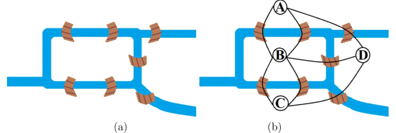
Given a set V and a set E such that E is composed of pairs of elements of V , we say that the pair (V, E) is a graph, where any element of V is called a vertex and any element of E is called an edge. The first known application of graphs was on the problem of the seven bridges of Königsberg formulated by Euler in the 18th century [30]. The problem was to determine if there exists any path that passes by all seven bridges (see Figure 1.1(a)) exactly once in such a way that the river can only be crossed through one of the bridges. Euler solved this problem using a graph representation of those bridges: each land area is represented by a vertex and each bridge is represented by an edge linking a pair of land areas, as shown in Figure 1.1(b). He proved that there is no solution to this problem. Furthermore, Euler demonstrated that the existence of a solution to other similar problems depends only on the topology of the underlying graphs rather than on the absolute geometrical positions of the bridges.
Since then, numerous optimization problems have been formulated in the framework of graphs. For instance, let us consider shortest path optimization problems. Let (V, E) be a graph and let x and y be two vertices in V . A path from x to y (in (V, E)) is a sequence (x1, . . . , x`) such that x1 = x, x` = y and such that, for i in {1, . . . , ` − 1}, the
edge {xi, xi+1} is an edge in E. If there is a path from x to y in (V, E), we say that x
and y are connected for (V, E). A shortest path from x to y is a path (x1, . . . , x`) such
that ` is minimal among all paths from x to y. In practice, a vertex can represent a “real object” as a city or an antenna, or an “abstract object” such as a word in a given language or profiles of a social network. Hence, edges can link neighbouring cities, closest pairs of antennas, similar words or virtual friends/followers. In this context, solving the
(a) (b)
Figure 1.1: (a): The configuration of the seven bridges of Königsberg in the 18th century. (b): The representation of the seven bridges of Königsberg as a graph.
shortest path problem can help with finding the most direct path between any two cities or antennas, the least number of modifications needed to transform one word into another, or to infer “how close are two users of a social network?”.
More complex problems can be formulated by assigning weights to the edges of a graph. Let G = (V, E) be a graph and let w be a map from E into the set of positive real numbers R+. For any edge u in E, we call w(u) the weight of u. We call (G, w)
a edge-weighted graph. In this context, the shortest path problem can be formulated so as to take into consideration the weights of the edges in E. Let f be any function from any path π = (x1, . . . , x`) into the set R+ of positive real numbers, e.g. f(π) =
max{w({xi, xi+1}) | i ∈ {1, . . . , ` − 1}} or f (π) = `
P
i=1
w({xi, xi+1}). Given any two
vertices x and y in V , a shortest path from x to y is a path π = (x1, . . . , x`) from x
to y such that f(π) is minimal among all paths from x to y. Considering the examples given in the previous paragraph, the weight of an edge can represent, for example, a road length, the time to transfer a given amount of data between two antennas, the level of similarity between two words or the number of interactions between two users of a social network. Hence, incorporating weights to the edges of a graph aids to approximate the graph representation to the real world problems.
As the problems aforementioned, the large literature on graph theory invites many classification problems to be formulated in the framework of graphs. We denote by class or cluster a group of (data) points which are similar with respect to a given criterion. Let P be a set. A classification of the elements of P is the assignment of each element of P to a class (or to several classes). In the context of graphs, the set P is formalized as the set of vertices of a graph, whose edges link pair of vertices that are potentially in the same class. Let(G, w) be a edge-weighted graph. A classification of the vertices of G
15
is often obtained by minimizing energy functions related to the weight of edges linking vertices in the same class (or edges linking vertices in different classes). For instance, let us consider that the vertices of G represent the researchers in a given conference. We may be interested in classifying this group of researchers according to their specific area of interest. To do so, we could link each two researchers x and y by an edge whose weight is the number of articles in which x cites y plus the number of articles in which y cites x. We can infer that, in most cases, the researchers working on the same area are linked by edges of larger weights than the edges linking researchers in different areas. Hence, a classification of the vertices of G could be the result of maximizing (resp. minimizing) the sum of the edges linking vertices in a same class (resp. different classes).
We can consider two variants of the previous classification problem: (1) supervised classification: the areas of research are defined beforehand and samples of each class are used by the classification algorithm; and (2) unsupervised classification: the areas of research are deduced from the result of the classification algorithm.
Similarly to classification problems, segmentation problems are also commonly formu-lated in the framework of graphs. Let P be a set. A segmentation of P is a partition of P into disjoint subsets R1, . . . , R` such that every element of P is in exactly one subset Ri.
Each subset of a segmentation of P is called a region of this segmentation. In practice, the set P represents a set of real or abstract objects whose similarity can be measured. Then, the elements of P are segmented by their degree of similarity. We can observe that classification and segmentation problems are related: a classification of the elements of P into disjoint classes induces a partition of P and, on the other hand, segmenting P can be a pre-processing step to classification algorithms, which is often the case. As classification problems, we can also consider two variations of segmentation methods: (1) marker-based segmentation: given a set S of disjoint subsets (markers) of P , each region of the final segmentation of P includes exactly one element of S; and (2) no markers are provided and the final regions depend on the algorithm and possibly on other parameters such as number and size of regions.
A typical segmentation problem is the segmentation of digital images. A (digital) image is a matrix of picture elements or pixels such that each pixel comprises the color or gray-scale information of a point in the image. Let I be an image. In the framework of edge-weighted graphs, the image I can be represented as an edge-weighted graph (G, w) such that the vertices of G correspond to the pixels of I, the edges of G link neighbouring pixels of I, and the edge weights are a measure of dissimilarity between pixels. Alterna-tively, the vertices of G can also represent disjoint subsets of connected pixels of I, with the resulting graph known as a Region Adjacency Graph (RAG).
Several notions related of graphs induce good solutions for practical image segmen-tation problems. Hence, we can profit of the efficient algorithms that have already been developed in graph theory in order to solve new application problems. To give an exam-ple, let us consider the minimum spanning forest problem. Let ((V, E), w) be a graph and let S be a set of disjoint subsets of the vertex set of G. A minimum spanning forest of ((V, E), w) rooted in S is a graph ((V, E0), w) such that:
1. any two vertices in a same element of S are connected for (V, E0);
2. any two vertices in distinct elements of S are not connected for (V, E0); and
3. the sum of the weight of all edges in E0is minimal for all graphs for which statements 1 and 2 hold true.
In the context of image segmentation, we can see that the minimum spanning forest of ((V, E), w) rooted in S induces a marker-based segmentation in which the regions are determined by the vertices (pixels) that are connected in (V, E0). As we will see
later, the notion of minimum spanning forests induce efficient segmentation algorithms which satisfy relevant mathematical properties. Moreover, minimum spanning forests are closely related to the segmentation method explored in this thesis: the watershed transform.
In the late 70’s, the watershed transform was proposed as a powerful tool in the seg-mentation of gray-scale digital images. Since then, numerous definitions and algorithms to implement the watershed transform have been designed. The idea behind the water-shed transform is that an image (or a weighted graph) can be visualized as a topographic surface. In this context, a set of connected pixels surrounded by pixels of strictly greater gray values (or a set of adjacent vertices/edges surrounded by vertices/edges of strictly greater weights) is a regional minimum of the surface. Each regional minimum can be associated to a zone of influence, known as a catchment basin. From any point x (pixel or vertex) in the zone of influence of a regional minimum, there is a descending path from x to this regional minimum, where a descending path is either defined as a sequence of connected pixels of non-increasing gray levels, or a sequence of vertices connected by edges of non-increasing weights.
By iteratively merging the regions of a segmentation, we produce a hierarchy of seg-mentations, which is a sequence of nested segmentations of an image. Hence, a hierarchy provide segmentations of an image with different levels of detail, where the segmentation in the lowest level contains the largest number of regions. When the initial segmentation
17
is a watershed segmentation of a graph and when the merging steps are guided by a sequence of minima of this graph, we obtain a hierarchical watershed.
When formalized in the framework of weighted graphs, hierarchical watersheds are deeply linked to the optimization problem of minimum spanning trees. As a result of this link, each segmentation of a hierarchical watershed is optimal in the sense of minimum spanning forests, providing us good quality hierarchy of segmentations that optimizes a well defined objective function. Moreover, minimum spanning tree algorithms can be adapted to the computation of hierarchical watersheds, which leads to efficient algorithms to compute the latter.
Hierarchical watersheds are part of a broader family of hierarchical image representa-tions, whose main applications include image simplification and filtering, implementation of morphological connected operators, and provision of a larger search space for object detection tasks (when compared to a single segmentation).
In this work, we study hierarchical watersheds in the framework of graphs. For visu-alization and evaluation purposes, we recur to the problem of digital image segmentation. However, the theoretical results introduced in this manuscript hold for arbitrary graphs and, hence, can be applied to a broader range of problems.
The remainder of this manuscript is organized as follows:
• Chapter 2 introduces the background theory of this research. We present a brief survey and the formal definitions related to each of those topics: hierarchical image representations, weighted graphs, connected hierarchies, saliency maps, morpholog-ical hierarchies (quasi-flat zones hierarchies, binary partition trees and hierarchmorpholog-ical watersheds), and attribute based hierarchies.
• Chapter 3 proposes a characterization of hierarchical watersheds and an efficient al-gorithm to recognize hierarchical watersheds. Using the notions of saliency map and binary partition hierarchy by altitude ordering (a special case of binary partition trees), we present a necessary and sufficient condition for any connected hierarchy to be a hierarchical watershed.
• Chapter 4 presents the watersheding operator, which converts any hierarchy into a hierarchical watershed of a given weighted graph. This operator is idempotent and its set of fixed points is precisely the set of hierarchical watersheds. Hence, we establish the link between the watersheding operator and the problem of recogniz-ing of hierarchical watersheds studied in Chapter 3. We also present an efficient algorithm that implements the watersheding operator and experimental results on images.
• Chapter 5 studies the probability of hierarchical watersheds. By definition, a hi-erarchical watershed can be computed from a sequence of minima of a weighted graph. In this chapter, we demonstrate that a hierarchical watershed can be ob-tained from numerous sequences of minima of a graph. We show that the number of sequences of minima associated to different hierarchical watersheds of a weighted graph may differ. In this context, we define the probability of a hierarchical wa-tershed with respect to the number of sequences of minima that could be used to compute this hierarchy. Then, we present an efficient method to obtain the prob-ability of a hierarchical watershed, and a characterization of the most and least probable hierarchical watersheds of a weighted graph.
• Chapter 6 introduces an evaluation framework of hierarchies of segmentations. We present three evaluation measures that summarize several aspects of a hierarchy of segmentations, including the tendency to over and under-segmentation, and the easiness of extracting objects of interest with the help of markers. This evaluation framework allows us to identify a hierarchical watershed based on a novel extinction value that outperform the classical area, dynamics and volume based hierarchical watersheds. Then, this evaluation framework is used to compare hierarchical wa-tersheds with other morphological hierarchies.
• Chapter 7 presents theoretical and experimental results of combinations of archical watersheds. We first perform a visual inspection of combinations of hier-archies. Then, using the evaluation framework introduced in Chapter 6, we show that combinations of hierarchical watershed through their saliency maps can outper-form the input hierarchies. We also study properties of combinations by providing a sufficient condition for a combination to always output a flattened (simplified) hi-erarchical watershed. Then, we present experimental results with the algorithm to recognize hierarchical watersheds (Chapter 3) applied to combinations of hierarchi-cal watersheds. Finally, we show the interest of applying the watersheding operator (Chapter 4) to combinations of hierarchical watersheds: evaluation scores at least as good as the combinations with the advantage of preserving the mathematical properties of hierarchical watersheds.
19
The results presented in this manuscript have been partially published in the following articles:
Conference proceedings:
• D. S. Maia, A. de Albuquerque Araujo, J. Cousty, L. Najman, B. Perret, and H. Talbot. Evaluation of combinations of watershed hierarchies. In International Symposium on Mathematical Morphology and Its Applications to Signal and Image Processing, pages 133–145. Springer, 2017.
• D. S. Maia, J. Cousty, L. Najman, and B. Perret. Recognizing hierarchical water-sheds. In International Conference on Discrete Geometry for Computer Imagery, pages 300–313. Springer, 2019.
• D. S. Maia, J. Cousty, L. Najman, and B. Perret. Watersheding hierarchies. In In-ternational Symposium on Mathematical Morphology and Its Applications to Signal and Image Processing, pages 124–136. Springer, 2019.
• D. S. Maia, J. Cousty, L. Najman, and B. Perret. On the probabilities of hierar-chical watersheds. In International Symposium on Mathematical Morphology and Its Applications to Signal and Image Processing, pages 137–149. Springer, 2019. Journals:
• B. Perret, J. Cousty, S. J. F. Guimaraes, and D. S. Maia. Evaluation of hierarchical watersheds. IEEE Transactions on Image Processing, 27(4):1676–1688, 2017. • D. S. Maia, J. Cousty, L. Najman, and B. Perret. Properties of combinations of
hierarchical watersheds. Under review. 2019.
• D. S. Maia, J. Cousty, L. Najman, and B. Perret. Characterization of graph based hierarchical watersheds: theory and algorithm. Under review. 2019.
Chapter 2
Hierarchies and Graphs
In this chapter, we present the background theory that led to the development of this thesis. We review graphs and hierarchies of partitions, in particular the family of hierarchies used in this research: quasi-flat zones hierarchies, binary partition trees, hierarchical watersheds and attribute based hierarchies.
Remark. The notations presented in this chapter are used all along the manuscript.
2.1
Graphs
A graph is a pair G = (V, E), where V is a finite set and E is a set of pairs of distinct elements of V , i.e., E ⊆ {{x, y} ⊆ V | x 6= y}. Each element of V is called a vertex (of G), and each element of E is called an edge (of G). To simplify the notations, the set of vertices and edges of a graph G will be also denoted by V(G) and E(G), respectively. Let G= (V, E) be a graph and let X be a subset of V . A sequence π = (x0, . . . , xn)
of elements of X is a path (in X) from x0 to xn if {xi−1, xi} is an edge of G for any i
in {1, . . . , n}. Given a path π = (x0, . . . , xn) from a vertex x0 to a vertex xn in V , for
any edge u = {xi−1, xi} for any i in {1, . . . , n}, we say that u is an edge in π. The
subset X of V is said to be connected (for G) if, for any x and y in X, there exists a path from x to y. The subset X is a connected component of G if X is connected and if, for any connected subset Y of V , if X ⊆ Y , then we have X = Y . In the following, we denote by CC(G) the set of all connected components of G.
Let G be a graph. If w is a map from the edge set of G to the set R of real numbers, then the pair (G, w) is called an (edge) weighted graph (see Figure 2.1(a)). If (G, w) is a weighted graph, for any edge u of G, the value w(u) is called the weight of u (for w).
We say that the graph G = (V, E) is a forest if, for any edge u in E, the number of 21
a b c d e f g h 1 1 1 1 2 3 2 (a) {a} {b} {c} {d} {e} {f } {g} {h} P 0 X1 X2 X3 X4 P1 X5 X6 P2 X7 P3 (b)
Figure 2.1: (a): A weighted graph (G, w). (b): A representation of a hierarchy of partitions H= (P0, P1, P2, P3) on the set {a, b, c, d, e, f, g, h}.
connected components of the graph (V, E \ {u}) is greater than the number of connected components of G. Given another graph G0, we say that G0 is a subgraph of G, denoted by G0 v G, if V (G0) is a subset of V and E(G0) is a subset of E. Let G00 be a subgraph
of G and let G0 be a subgraph of G00. The graph G00 is a Minimum Spanning Forest (MSF) of G rooted in G0 if:
1. the graphs G and G00 have the same set of vertices, i.e., V(G00) = V ; and
2. each connected component of G00 includes exactly one connected component of G0; and
3. the sum of the weight of the edges of G00 is minimal among all subgraphs of G for which the above conditions 1 and 2 hold true.
A MSF of (G, w) rooted in a single vertex of G is a tree (connected forest) called a Minimum Spanning Tree (MST) of (G, w).
Let (G, w) be a weighted graph and let k be a value in R. A connected subgraph G0 of G is a (regional) minimum (of w) at level k if:
1. the set of edges E(G0) of G0 is not empty; and
2. for any edge u in E(G0), the weight of u is equal to k; and
3. for any edge {x, y} in E \ E(G0) such that |{x, y} ∩ V (G0)| ≥ 1, the weight of {x, y}
is strictly greater than k.
2.2
Hierarchies of partitions
In this section, we first introduce notations and definitions related to hierarchies of par-titions. Then, we review partitions and hierarchies of partitions in the context of digital
2.2. Hierarchies of partitions 23
image processing and analysis.
2.2.1
Notations and definitions
Let V be a set. A partition (of V ) is a set P of non empty disjoint subsets of V whose union is V . Any element of a partition P is called a region of P. Let P1 and P2 be two
partitions. We say that P1 is a refinement of P2 if every element of P1 is included in an
element of P2. A hierarchy (of partitions) is a sequence H = (P0, . . . , P`) of partitions
such that Pi−1 is a refinement of Pi, for any i in {1, . . . , `} and such that Pn = {V }.
Let H = (P0, . . . , P`) be a hierarchy of partitions. Any region of a partition P of H is
called a region of H. The set of all regions of H is denoted by R(H).
A hierarchy of partitions can be represented as a tree whose nodes correspond to regions, as shown in Figure 2.1(b). Given a hierarchy H and two regions X and Y of H, we say that X is a parent of Y (or that Y is a child of X) if Y ⊂ X and X is minimal for this property, i.e., if there is a region Z such that Y ⊆ Z ⊂ X, then we have Y = Z. It can be seen that any region X 6= V of H has exactly one parent. For any region X such that X 6= V , we write parent(X) = Y where Y is the unique parent of X. For any region R of H, if R is not the parent of any region of H, we say that R is a leaf region (of H). Otherwise, we say that R is a non-leaf region (of H).
We illustrate a hierarchy of partitions H in Figure 2.1(b). The regions of the hierar-chy H are represented by nodes on a tree. Each region of H is linked to its parents (and to its children) by straight lines.
Let G= (V, E) be a graph. A partition of V is connected for G if each of its regions is connected and a hierarchy on V is connected (for G) if every one of its partitions is connected. For example, the hierarchy of Figure 2.1(b) is connected for the graph of Figure 2.1(a).
2.2.2
Partitions in the context of digital images
A digital image is a numeric representation of an image: a matrix or set of picture elements or pixels, where each pixel carries the colorimetric information of a point in the image (see Figure 2.2). The information associated to each pixel varies depending on the nature of the image representation. In gray-scale images, a pixel can be associated to a single value that indicates the gray-level of this pixel - brighter pixels being assigned to greater values. In turn, a pixel of a color image can be represented as a combination of the levels of red (R), blue (B) and green (G) colors in this pixel. The latter representation corresponds to a vector in the RGB color space.
Figure 2.2: A gray-scale and a color image.
Figure 2.3: An image I and a partition of I into two regions.
Let I be an image and let {p0, . . . , pn} be the set of pixels of I. A partial partition of I
is a set of disjoint subsets of {p0, . . . , pn}. A (total) partition or segmentation of I is a set
of disjoint subsets of {p0, . . . , pn} such that every pixel of I belongs to an element of this
partition. Each element of an image partition is called a region of this partition. Along this manuscript, the terms partition and segmentation will be used interchangeably. An image segmentation is illustrated in Figure 2.3.
The need for image segmentation arose with the various applications of digital images in research fields such as biology, medicine and astronomy. Image segmentation is usu-ally a pre-processing step to other image processing and analysis tasks, including image filtering and simplification, object detection, object tracking and scene labeling. As the size of images to be processed increases, manual segmentation becomes an onerous task. In the early days of image segmentation, heuristic techniques for image segmentation have been employed. For instance, we can cite low-level pixels classification techniques such as thresholding and histogram analysis, in which pixels are segmented based solely on their colorimetric information.
2.2. Hierarchies of partitions 25
arbitrary sets of points based on the distance between those points. When applied to image segmentation, this technique takes into consideration not only the local information of a pixel but also its position with respect to other similar pixels. Following a similar idea, the authors of [35] propose a greedy graph-based segmentation method that relies on the dissimilarity between pixels of a region and on the dissimilarity between neighbouring regions of a segmentation. The latter method uses a greedy approach to optimize a global energy, which is also the case of the segmentation technique investigated in this research: the watershed transform.
The watershed segmentation was first studied in [12] and, since then, numerous def-initions have been proposed [2, 22]. The idea underlying this technique is that a node (vertex) or edge weighted graph can be visualized as a topographic surface in which the node and edge weights determine the altitude of the points on the surface. In geogra-phy, a catchment basin is a region whose collected water drain to a common point (e.g. a sea), and the watersheds are the dividing lines between neighbour catchment basins. Each catchment basin is associated to a regional minimum, which is a plateau surrounded by points of greater altitude. A point in the surface belongs to a given catchment basin if there exists a descending path from this point to the regional minimum in this catch-ment basins. In the context of node and edge weighted graphs, a regional minimum is a subgraph (or a subset of vertices) of uniform weight and surrounded by nodes or edges of greater weights. The watershed transform segments the vertices of a weighted graph into its catchment basins. This idea can be applied to the segmentation of gray-scale images by either computing an image gradient represented as a weighted graph or by consider-ing that the altitudes of the topographic surface are given by the pixel gray-levels. More details on the watershed segmentation are given later in Section 2.6.
Image segmentation is an ill-posed problem as it does not have a fixed optimal so-lution for all applications. Still, efforts have been made to establish ground-truths for large image datasets, which can be further used as a reference to image segmentation algorithms. Such datasets include the Berkeley Segmentation Dataset and Benchmark (BSDS500) [63], Grabcut [16], Weizman [1], Pacal Context [71] and COCO [54].
2.2.3
Hierarchies of partitions in the context of digital images
As stated in the previous section, there is no global optimal segmentation of an image. For different tasks, segmentations with distinct levels of detail may be required. In this context, hierarchies of image segmentations arise as an all-purpose tool for image segmen-tation. More generally, hierarchies of image segmentations are part of a broader group of hierarchical image representations, which also include hierarchies of partial partitions
and inclusion hierarchies. As discussed later in this section, the use of hierarchical image representations goes beyond image segmentation.
In the remainder of this section, we review well-known hierarchical image representa-tions and their applicarepresenta-tions.
Since the early work of [78] on a splitting and merging hierarchical partition al-gorithm, several methods to compute and process hierarchies of partitions have been proposed. Among the image processing tasks aided by hierarchies of partitions, we cite image simplification, filtering, and segmentation.
In [13], the author propose an algorithm, called waterfall algorithm, to overcome the oversegmentation resulting from watershed segmentations. In his algorithm, the initial regions of a watershed segmentation are iteratively merged until a simplified segmenta-tion is obtained. The intermediate segmentasegmenta-tions produced by this method compose a hierarchy of partitions.
In [48], the authors proposed a hierarchical segmentation method based on the graph-based segmentation introduced in [35]. The algorithm proposed in [35] receives as input a parameter to control the size of regions and the dissimilarity between the regions of the resulting segmentation. As the causality and location properties do not hold for the segmentations produced by [35] using increasing parameters, the authors of [48] propose an adaptation of this method.
In the family of morphological hierarchies with large applications to image filtering and simplification, we can cite min-trees, max-trees, tree of shapes, quasi-flat zones hierarchies, binary partition trees and hierarchical watersheds [72, 13, 87, 65, 24, 27, 74], which will be explored next.
Let I be a gray-scale image. A level-set of I is a subset of the pixels of I with gray values greater than a given threshold parameter λ. Any gray-scale image can be equally represented by its level-sets. The min-tree and max-tree are dual representations of the level-sets of an image: the max-tree of an image I is composed of the connected components of the level-sets of I while that the min-tree of I is composed of the connected components of the complement of the level-sets of I. Therefore, the leaf regions of a max-tree (resp. min-max-tree) are the regional maxima (resp. minima) of an image. Those max-trees are widely used in the implementation of connected operators [88, 89], the max-tree (resp. min-tree) being useful to compute anti-extensive (resp. extensive) operators.
Let I be a gray-scale image. A flat zone of I is a maximal connected set of pixels of I with uniform gray values. Connected operators act by removing flat-zones and, therefore, do not create any new contours in the image. A quasi-flat zone is a connected set of pixels whose gray-level difference of neighbouring pixels is limited by a given value threshold λ.
2.2. Hierarchies of partitions 27
A quasi-flat zone hierarchy is a sequence of segmentations composed of flat-zones of an image with increasing values for the parameter λ. In the context of edge-weighted graphs, a quasi-flat zone is a connected set of vertices such that the difference between the weight of any two adjacent edges is limited to a given value λ. The connection between quasi-flat zone hierarchies and other morphological hierarchies has been studied in [27]. Moreover, quasi-flat zones hierarchies are linked to a dual representation of hierarchies of partitions known as saliency maps, which is explained later in Section 2.4.
The tree of shapes [65] is a hierarchical image representation based on the inclusion relationship between the connected components of the level-sets (and of the complement of the level-sets) of an image. They are self-dual and contrast-invariant. Furthermore, the tree of shapes is a compact representation of the max-tree and min-tree of an image since any region of those two hierarchical representations can be found in the tree of shapes. Properties and applications of the tree of shapes have been studied in [104] and an efficient algorithm to obtain a tree of shapes is given in [39].
Binary partitions trees were first proposed by Salembier and Garrido [87] as a tool for simplifying, segmenting and extracting information from images. The construction of this hierarchy relies on the notions of merging order, merging criterion and region model. Given any segmentation P, a binary partition hierarchy is constructed by merging the regions of P following a given merging order defined on the regions of P. Each region built along this process is represented according to a region model as, for example, the average gray-level of the pixels belonging to a region. The merging criterion, e.g. the color homogeneity between two regions, determines if any two neighbouring regions should be merged. Particular cases of this hierarchy have been studied under several names, such as α-tree [77] and binary partition hierarchy by altitude ordering [27]. An extension of binary partition hierarchies applied to multiple images and multiple criteria was proposed in [86].
Outside the group of morphological hierarchies, several high-quality hierarchical seg-mentation methods have been proposed [5, 7, 60].
In [5], the authors introduce a multiscale contour detector that combines multiple contour cues: brightness, color and texture gradient. Then, the output of their contour detector is used to obtain a segmentation through their method called oriented watershed transform. The oriented watershed transform outputs weighted boundaries which are further used to compute a hierarchy of partitions.
In [7], the authors propose a hierarchical segmentation method based on the combi-nation of hierarchies computed from different resolutions of the same image. For each resolution, they compute the normalized cuts of the image contours, which are based on
the same contour cues used by [5]. Then, those normalized cuts are combined into a single Ultrametric Contour Map (UCM), which is a dual representation of a hierarchy of partitions and also known as a (contour) saliency map. Finally, they align the UCMs obtained at different resolutions into a single UCM.
In [60], the authors propose a hierarchical segmentation method using Convolutional Neural Networks (CNN). Each level of a CNN conveys information regarding different levels of resolution of an image. Hence, the authors use the output of each level of a CNN to compute oriented boundaries and, subsequently, UCMs. The UCMs obtained at different levels are further aligned using a faster implementation of the method proposed in [7], producing hierarchies with state-of-the-art performance in several computer vision applications.
With so many algorithms to compute hierarchies of partitions, it became necessary to evaluate the contribution of each hierarchy with respect to different tasks [5, 83, 82, 79]. Usually, large annotated image datasets are used to evaluate hierarchical segmentation algorithms. Those evaluations are often empirical in the sense that an algorithm is eval-uated with respect to its output on a set of images. As the manual annotations provided by large image datasets [63, 16, 1, 71] are not hierarchical, hierarchies of partitions are commonly evaluated by comparing each segmentation of the hierarchy against the image ground truth.
Aiming at expanding the search space of image segmentation problems, the notion of hierarchies of partitions is extended to braids of partitions in [53]. A braid of partitions is composed of partitions that locally follow the causality and location principles: given any two partitions P1and P2 of a braid of partitions, every region of P1 is either a subset
of a region of P2 or it is composed of regions of P2. Hence, any hierarchy of partitions
is a braid of partitions but the other implication is not true in general.
Several well-known image segmentation techniques are modeled in the framework of graphs [17, 90, 35, 31, 43, 21], including (hierarchical) watersheds [66, 22, 24, 27, 74]. In this thesis, we focus on morphological hierarchies built in the framework of weighted graphs and, in particular, on hierarchical watersheds and on their link with other morphological hierarchies such as the binary partition trees.
2.3
Quasi-flat zones hierarchies
In this section, we first present the definition of quasi-flat zone hierarchy in the framework of weighted graphs. Then, we present some of the applications of quasi-flat zones in the context of image segmentation.
2.3. Quasi-flat zones hierarchies 29
2.3.1
Notations and definitions
Let(G, w) be a weighted graph and let λ be any element in R. Let V and E be the vertex and edge sets of G, respectively. The λ-level set of (G, w) is the graph (V, Eλ(G)) such
that Eλ(G) = {u ∈ E(G) | w(u) ≤ λ}. Without loss of generality, let us assume that the
range of w is included in the set E of all integers from 0 to |E| − 1 (otherwise, one could always consider an increasing one-to-one correspondence from the set {w(u) | u ∈ E} into the subset {0, ..., |{w(u) | u ∈ E}| − 1} of E). The sequence
QF Z(w) = (CC(Gλ,w) | λ ∈ E) (2.1)
where Gλ,w is the λ-level set of (G, w), is a hierarchy called the Quasi-Flat Zones (QFZ)
hierarchy (of w) [72, 69, 92, 27].
For instance, the hierarchy H of Figure 2.1(a) is the QFZ hierarchy of the graph(G, w) of Figure 2.1(b).
2.3.2
Quasi-flat zones for image segmentation
Let I be a gray-scale image such that the gray value of any pixel of I is in the range[0, 255]. A flat-zone of I is a set of connected pixels (e.g. 4 or 8 connected pixels) with uniform gray-level. In the context of edge weighted graphs, a flat zone is a set of vertices linked by edges with uniform weight. Let k be a value in [0, 255]. The k-level set of I is the set of pixels of I with gray-levels greater than k. Any gray-scale image can be equally represented and reconstructed from its level sets.
Connected operators act on the connected components of the level sets of an image (or on the complement of the level sets of an image). Hence, connected operators filter out or merge connected components of the level sets of an image without creating new contours, which is very useful for image simplification. As mentioned in Section 2.2.3, connected operators can be implemented through hierarchical representations of an image, including min-tree, max-tree and tree of shapes.
A quasi-flat zone of an image is a largest set of connected pixels such that the difference in gray-level between two neighbour pixels is limited by a given threshold k. For any k, we can define a partition of the image. By stacking the partitions of quasi-flat zones of an image for increasing values of k, we obtain a sequence of partitions for which the causality and location properties hold true, resulting in the quasi-flat zones hierarchy. From this definition, we can infer two features of flat zones partitions. First, quasi-flat zones partitions are prone to connect dissimilar regions that are linked only by a
narrow path (leakage problem). Second, dissimilar regions can be connected by a path in which gray-levels vary smoothly (chaining problem).
The first use of quasi-flat zones dates back to [72] in the analysis of aerial photographs. In order to segment and classify regions of aerial images into forest, cropts, houses, etc., the authors use the quasi-flat zones of the smoothed images for a given threshold, along with colorimetric and geometric information.
In [92], the author addresses the chaining problem of quasi-flat zones, where pixels of large gray-level difference are connected by a path of low gray-level variation between neighbouring pixels. As a solution to this issue, he proposes the introduction of a new parameter to control the maximal gray-level variation between pixels of a same region. They denote quasi-flat zones as α-connected components.
In [69], the authors introduce a morphological scale space representation of images based on the notion of levelings. A function g is a leveling of a function f if, for any two neighbouring pixels x and y, we have that g(x) > g(y) implies that f (x) ≥ g(x) and g(y) ≥ g(x). They prove that levelings are connected filters, hence the link with quasi-flat zones. They show that, as quasi-flat zones, levelings with increasing parameters lead to a hierarchical representation of an image obeying the causality and location principle of the regions and contours.
In [27], the authors link quasi-flat zones hierarchies with other morphological hierar-chies in the context of weighted graphs. They show that a quasi-flat zone hierarchy can be obtained by simplifying a binary partition tree. In particular, quasi-flat zones hierar-chies are linked to saliency maps, which are a compact representation of hierarhierar-chies of partitions, as discussed in the next section.
2.4
Contour saliency maps
Until now, we have considered hierarchies of partitions represented by the inclusion re-lationship between regions or by a sequence of partitions. In this section, we introduce a dual representation of hierarchies of partitions. Instead of a sequence of partitions, we characterize a hierarchy of partitions by the contours between the regions of each partition. As established in [25], a connected hierarchy can be equivalently treated by means of a weighted graph through the notion of a (contour) saliency map (also known as ultrametric contour map [5]). A saliency map is a map from the contours present in the partitions of a hierarchy into a set of values indicating the level of disappearance of each contour. Through the definition of quasi-flat zones, any hierarchy can be recovered from its saliency map.
2.4. Contour saliency maps 31
Saliency maps and hierarchies are closely related to the notion of ultrametric dis-tances [73, 5]. An ultrametric distance is a metric space that satisfies the ultrametric inequality: given an ultrametric distance map d and three points x, y and z in the space, we have d(x, y) ≤ max{d(x, z), d(z, y)}. Given a hierarchy H = (P0, . . . , P`) on a set V ,
let f be a function from V × V into the set {0, . . . , `} such that, for any two vertices x and y in V , f(x, y) is the lowest k such that x and y belong to the same region of Pk.
We can observe that:
• for any x in V , f (x, x) = 0; and
• for any x and y in V , f (x, y) ≥ 0 and f (x, y) = f (y, x); and
• for any x, y, z in V , f (x, y) ≤ max{f (x, z), f (z, y)} because the level in which x and y belong to the same region is necessarily finer than the level in which x, y and z belong to the same region.
Hence, f is an ultrametric distance and we can see that the hierarchy H can be recovered from f . Indeed, if H is connected for a given graph G, the values of f for the edges of G suffice to recover the hierarchy H. This map f0 from the edges of E into their value in f is the saliency map of H. The reader may note that, in other contexts, a saliency map denotes a map that highlights the objects of interest of an image (high values for pixels belonging to important regions), which is not our case. Here, the saliency values are assigned to the contours and not to the interior of the regions.
The first definition of saliency maps in the context of hierarchies of partitions was presented by Najman and Schmitt [75]. In [75], the authors extend the definition of dynamics of minima [45] to dynamics of contours. They define a map from each contour of a watershed segmentation into the saliency of this contour, where any threshold of the resulting map produces closed contours.
In this work, we focus on connected hierarchies. Let G be a graph and let H be a hierarchy connected for G. The saliency map of H is defined on the edges of G because all vertices of G belong to a region of H. In this context, saliency maps are represented thanks to cubical complexes [26]: the representation of a saliency map is an image with the double number of lines and columns of the original image and where every vertex and every edge is represented by a pixel.
In Figure 2.4, we show a representation of a saliency map. In this representation, the darkest contours are the ones that persist at the highest levels of the hierarchy.
(a) I (b) f
Figure 2.4: An image I and the saliency map f of a hierarchy of partitions of I obtained with the method proposed in [60].
2.4.1
Notations and definitions
Let G= (V, E) be a graph. Given a hierarchy H = (P0, . . . , P`) which is connected for G,
the (contour) saliency map of H is the map from E into {0, . . . , `}, denoted by Φ(H), such that, for any edge u= {x, y} in E, the value Φ(H)(u) is the lowest value i in {0, . . . , `} such that x and y belong to a same region of Pi. It follows that any connected hierarchy
has a unique saliency map. Moreover, any hierarchy H connected for G is precisely the quasi-flat zones hierarchy of its own saliency map: H= QFZ(Φ(H)).
For instance, the map depicted in Figure 2.1(b) is the saliency map of the hierarchy of Figure 2.1(a).
Let G= (V, E) be a graph and let H = (P1, . . . , P`) be a hierarchy on V . Let d be a
map from V ×V into R such that, for any pair (x, y) of vertices in V ×V , the value d(x, y) is the greatest edge weight λ in a path π from x to y (resp. y to x) in (G, Φ(H)) and such that, for any other path π0 from x to y (resp. y to x), the greatest edge weight in π0 is greater than or equal to λ. For any egde u = {x, y} in E, we say that d(x, y) is the ultrametric distance between x and y in (G, Φ(H)). We can affirm that (V, d) is an ultrametric space. Moreover, for any two vertices x and y in V , by the definition of saliency maps and considering its link with QFZ hierarchies, we may say that d(x, y) is the lowest value λ such that x and y belong to a same region of the partition Pλ of H.
Furthermore, if G is a complete graph, we can conclude that (V, Φ(H)) is an ultrametric space.
2.5. Binary partition trees 33
2.5
Binary partition trees
Binary partition trees [87] are widely used for hierarchical image representation. In this section, we first review the definition of binary partition tree and some of its applica-tions. Then, we describe the particular case where the merging order is defined by the edge weights [27]. As we will see along this manuscript, the latter is deeply connected to hierarchical watersheds [27] and can be used to study properties of hierarchical water-sheds.
2.5.1
Introduction
In [87], the notion of binary partition tree (BPT) is introduced aiming to fuse the flex-ibility of the order in which regions are merged by segmentation algorithms and the flexibility offered by connected operators in the processing of the max-tree.
The execution of segmentation algorithms based on merging criteria involves three concepts: merging order, merging criteria and region model. Given an initial set of regions or superpixels, the merging order determines the order in which pairs of neighbouring regions should be considered for merging, which is given by the similarity between regions according to a given criterion, e.g. average gray level. The merging criterion determines when the merging process stops, e.g. when a given number of regions is reached. The region model determines how each region is represented after each merging step, e.g. average gray-level of the pixels in a region.
As discussed in Section 2.3, connected operators are operators that act on the con-nected components of the flat-zones of thresholded versions of an image. Given an im-age I and a connected operatorΨ, we can say that the partition induced by the flat-zones of Ψ(I) at level λ is coarser than the partition induced by the flat-zones of I. Connected operators can be efficiently implemented through max-trees: given a max-tree T , Ψ is a filtering of the regions of T according to a given criterion. When this criterion is in-creasing on the nodes of T , Ψ simply filters out all descendants of any region that does not follow the criterion. Otherwise, if the criterion is non increasing, the result is not robust in the sense that similar images can have different results. Strategies to handle non-increasing criteria are discussed [88].
A BPT as presented in [87] can be constructed through algorithms based on a merging criterion. The BPT is obtained by keeping track of the merging sequence of an algorithm, i.e., the sequence of pair of regions of a segmentation that are merged by a merging algorithm. The merging criterion is the merging of all initial regions into a single region. Then, the processing of a BPT follows the same pruning strategies used in the processing
of the max-tree by connected operators.
Among the applications of the BPT, Salembier and Garrido [87] highlight:
1. detection and recognition of regions based on a given criteria e.g. circularity. The BPT offers a set of 2N-1 regions (where N is the number of initial regions), which limits the search space to a small number of reasonably homogeneous regions; 2. image compression for low bandwidth servers. Instead of sending the color
informa-tion of each pixel individually, some regions of the image can be sent as a superpixel (only the contours and a constant color are sent). The distortion of the resulting image and the budget to send an image can be optimized on the BPT when both distortion and budged are increasing on the regions of the BPT; and
3. image segmentation. Image segmentations can be extracted from the BPT by simply following the merging order used to construct the BPT. The desired number of regions can be used as a merging criterion and the final segmentation can be obtained by filtering the BPT as done by connected operators on the max-tree. This latter approach is called direct segmentation. Alternatively, segmentations can be obtained by propagating markers from the leaves, at the pixel level, to the root. This marked segmentation technique has been notably used in the evaluation framework of hierarchies proposed in [80, 79] to be discussed in Chapter 6.
BPTs have been largely used in remote sensing image processing [99, 11, 86]. The advance in this area, leading to larger scale images, call for a method to efficiently simplify an image and to decrease the search space of the objects in a remote sensing image.
In [99], the authors segment hyperspectral images by applying a Support Vector Machine (SVM) to nodes of a BPT. Given a BPT computed from a hyperspectral image, the nodes of this BPT are classified by an SVM according to their impurity level, which is related to the number of different classes assigned to the descendants of a node. Then, this BPT is pruned and the class of each pixel is determined by the leaf region that contains this pixel. The authors show that a simple SVM classification is improved with the aid of a BPT.
In [86], the authors proposed a multi-criteria and multi-image binary partition tree computation with application to remote sensing image segmentation. They build a BPT from several photographs of the same scene. Then, they work on a set of images with the same dimensions, where each image induces a different dissimilarity graph (gradient) and the merging criterion is defined by alternating the information provided by each graph.
2.5. Binary partition trees 35
In [100], BPT is used for object detection with application to face and traffic sign detection. Using a merging criterion based on color and contour complexity, the authors study methods to obtain the initial partition of the BPT and the merging sequence separately.
In [27], the authors establish the link between BPTs, minimum spanning tree and other morphological hierarchies, in particular the min-trees, quasi-flat zones hierarchies and hierarchical watersheds. They introduce a particular case of the BPTs denoted by binary partition hierarchy by altitude ordering (BPHAO), which can be used to obtain QFZ hierarchies, min-trees and hierarchical watersheds. The link between BPHAO and hierarchical watersheds are the basis of our research on characterization of hierarchi-cal watersheds (see Chapter 3), on the watersheding operator (see Chapter 4) and on probabilities of hierarchical watersheds (Chapter 5).
BPHAOS are deeply related to single linkage clustering [42]. Hence, the link between MST and single linkage clustering established in [42] can be extended to BPHAOs. For example, MST algorithms have been successfully used by Najman et al. [74] to compute BPHAOs. The authors of [74] also provide an efficient post-processing of the BPT to find the minima and watershed-cut edges of a graph, as explained in Section 2.6.1.
In the next section, we formalize the definition of BPHAO in the framework of weighted graphs.
2.5.2
Notations and definitions
Let (G, w) be a weighted graph. Let V and E be the vertex and edge sets of G, re-spectively. Let ≺ be a total ordering (on E), i.e., ≺ is a binary relation that is transi-tive and trichotomous: for any u and v in E only one of the relations u ≺ v, v ≺ u and v = u holds true. We say that ≺ is an altitude ordering (on E) for w if, for any u and v in E, if w(u) < w(v), then u ≺ v. Let ≺ be an altitude order-ing for w. Let k be any element in {1, . . . , |E|}. We denote by u≺k the k-th el-ement of E with respect to ≺. We set B0 = {{x} | x ∈ V }. The k-partition
of V (by the ordering ≺) is defined by Bk = {Byk−1 ∪ Bxk−1} ∪ (Bk−1 \ {Bxk−1, B y k−1})
where u≺k = {x, y} and Bx
k−1 and B y
k−1 are the regions of Bk−1 that contain x and y,
respectively. The sequence (Bi | i = 0 or Bi 6= Bi−1) is a hierarchy on V . This
hierar-chy (Bi | i = 0 or Bi 6= Bi−1), denoted by B≺, is called the binary partition hierarchy
(by altitude ordering) of (G, w) by ≺.
Let B be a hierarchy on V . We say that B is a binary partition hierarchy (by altitude ordering) of (G, w) if there is an altitude ordering ≺ for w such that B is the binary partition hierarchy of (G, w) by ≺.
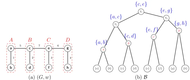
A B C D a b c d e f g h 1 2 3 4 5 7 6 (a) (G, w) {a} {b} {c} {d} {e} {f } {g} {h} A {a, b} B {c, d} C {e, f } D {g, h} Y5 {a, c} Y6 {e, g} Y7 {c, e} (b) B
Figure 2.5: (a): A weighted graph(G, w) with four minima delimited by the dashed lines. (b): The unique binary partition hierarchy B of (G, w).
Let ≺ be an altitude ordering for w. We can associate any non-leaf region X of the binary partition hierarchy B≺ of (G, w) by ≺ to the lowest rank r such that Br
contains X. This rank is called the rank of X. Let X be a non-leaf region of B≺ and let r
be the rank of X. The building edge of X is the r-th edge for ≺. Given an edge u in E, if u is the building edge of a region of B≺, we say that u is a building edge for ≺. Given
a building edge u for ≺, we denote the region of B≺whose building edge is u by Ru. The
set of all building edges for ≺ is denoted by E≺.
Let(G, w) be the weighted graph illustrated in Figure 2.5(a) and let B be the binary partition hierarchy of(G, w) illustrated in Figure 2.5(b). We can see that B is the binary partition hierarchy of (G, w) by the altitude ordering ≺ such that {a, b} ≺ {c, d} ≺ {e, f } ≺ {g, h} ≺ {a, c} ≺ {e, g} ≺ {c, e}. The building edge of each non-leaf region R of B is shown above the node that represents R.
Let B be a binary partition hierarchy of (G, w) and let X and Y be two distinct regions of B. If the parent of X is equal to the parent of Y , we say that X is a sibling of Y , that Y is a sibling of X and that X and Y are siblings. It can be seen that any region R 6= V of B has exactly one sibling and we denote this unique sibling of R by sibling(R).
2.6
Hierarchical watersheds
In this section, we first present the notations and definitions related to hierarchical wa-tersheds in the sense of minimum spanning forests [24, 27], and the link between
![Figure 2.4: An image I and the saliency map f of a hierarchy of partitions of I obtained with the method proposed in [60].](https://thumb-eu.123doks.com/thumbv2/123doknet/14564373.726664/37.892.241.615.157.441/figure-image-saliency-hierarchy-partitions-obtained-method-proposed.webp)
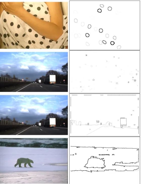
![Figure 4.5: First line from left to right: original image I and the gradient G of I computed using the edge detector introduced in [29]](https://thumb-eu.123doks.com/thumbv2/123doknet/14564373.726664/91.892.142.705.160.910/figure-right-original-image-gradient-computed-detector-introduced.webp)
![Figure 4.6: First line from left to right: original image I and the gradient G of I computed using the edge detector introduced in [29]](https://thumb-eu.123doks.com/thumbv2/123doknet/14564373.726664/92.892.142.805.287.749/figure-right-original-image-gradient-computed-detector-introduced.webp)