Genetic structure of fragmented southern populations of African Cape buffalo (Syncerus caffer caffer)

RESEARCH OUTPUTS / RÉSULTATS DE RECHERCHE

Author(s) - Auteur(s) :

Publication date - Date de publication :

Permanent link - Permalien :

Rights / License - Licence de droit d’auteur :

Bibliothèque Universitaire Moretus Plantin

Dépôt Institutionnel - Portail de la Recherche

researchportal.unamur.be

University of Namur

Genetic structure of fragmented southern populations of African Cape buffalo

(Syncerus caffer caffer)

Smitz, Nathalie; Cornélis, Daniel; Chardonnet, Philippe; Caron, Alexandre; de

Garine-Wichatitsky, Michel; Jori, Ferran; Mouton, Alice; Latinne, Alice; Pigneur, Lise Marie; Melletti,

Mario; Kanapeckas, Kimberly L.; Marescaux, Jonathan; Pereira, Carlos Lopes; Michaux,

Johan

Publisher's PDF, also known as Version of record

Link to publication

Citation for pulished version (HARVARD):

Smitz, N, Cornélis, D, Chardonnet, P, Caron, A, de Garine-Wichatitsky, M, Jori, F, Mouton, A, Latinne, A, Pigneur, LM, Melletti, M, Kanapeckas, KL, Marescaux, J, Pereira, CL & Michaux, J 2014, 'Genetic structure of fragmented southern populations of African Cape buffalo (Syncerus caffer caffer)', BMC Evolutionary Biology, vol. 14, no. 1, pp. 203. https://doi.org/10.1186/s12862-014-0203-2

General rights

Copyright and moral rights for the publications made accessible in the public portal are retained by the authors and/or other copyright owners and it is a condition of accessing publications that users recognise and abide by the legal requirements associated with these rights. • Users may download and print one copy of any publication from the public portal for the purpose of private study or research. • You may not further distribute the material or use it for any profit-making activity or commercial gain

• You may freely distribute the URL identifying the publication in the public portal ?

Take down policy

If you believe that this document breaches copyright please contact us providing details, and we will remove access to the work immediately and investigate your claim.

R E S E A R C H A R T I C L E

Open Access

Genetic structure of fragmented southern

populations of African Cape buffalo (Syncerus

caffer caffer)

Nathalie Smitz

, Daniel Cornélis

, Philippe Chardonnet

, Alexandre Caron

, Michel de Garine-Wichatitsky

,

Ferran Jori

, Alice Mouton

, Alice Latinne

, Lise-Marie Pigneur

, Mario Melletti

, Kimberly L Kanapeckas

,

Jonathan Marescaux

, Carlos Lopes Pereira

and Johan Michaux

Abstract

Background: African wildlife experienced a reduction in population size and geographical distribution over the last millennium, particularly since the 19thcentury as a result of human demographic expansion, wildlife overexploitation, habitat degradation and cattle-borne diseases. In many areas, ungulate populations are now largely confined within a network of loosely connected protected areas. These metapopulations face gene flow restriction and run the risk of genetic diversity erosion. In this context, we assessed the “genetic health” of free ranging southern African Cape buffalo populations (S.c. caffer) and investigated the origins of their current genetic structure. The analyses were based on 264 samples from 6 southern African countries that were genotyped for 14 autosomal and 3 Y-chromosomal microsatellites.

Results: The analyses differentiated three significant genetic clusters, hereafter referred to as Northern (N), Central (C) and Southern (S) clusters. The results suggest that splitting of the N and C clusters occurred around 6000 to 8400 years ago. Both N and C clusters displayed high genetic diversity (mean allelic richness (Ar) of 7.217, average

genetic diversity over loci of 0.594, mean private alleles (Pa) of 11), low differentiation, and an absence of an

inbreeding depression signal (mean FIS = 0.037). The third (S) cluster, a tiny population enclosed within a small

isolated protected area, likely originated from a more recent isolation and experienced genetic drift (FIS = 0.062,

mean Ar = 6.160, Pa = 2). This study also highlighted the impact of translocations between clusters on the genetic

structure of several African buffalo populations. Lower differentiation estimates were observed between C and N sampling localities that experienced translocation over the last century.

Conclusions: We showed that the current genetic structure of southern African Cape buffalo populations results from both ancient and recent processes. The splitting time of N and C clusters suggests that the current pattern results from human-induced factors and/or from the aridification process that occurred during the Holocene period. The more recent S cluster genetic drift probably results of processes that occurred over the last centuries (habitat fragmentation, diseases). Management practices of African buffalo populations should consider the

micro-evolutionary changes highlighted in the present study.

Keywords: Syncerus caffer caffer, Population genetics, Genetic structure, Translocation, Southern Africa, Conservation implications

* Correspondence:[email protected]

1

Departement of Life Sciences-Conservation Genetics, University of Liège, Liège, Belgium

Full list of author information is available at the end of the article

© 2014 Smitz et al.; licensee BioMed Central Ltd. This is an Open Access article distributed under the terms of the Creative Commons Attribution License (http://creativecommons.org/licenses/by/4.0), which permits unrestricted use, distribution, and reproduction in any medium, provided the original work is properly credited. The Creative Commons Public Domain Dedication waiver (http://creativecommons.org/publicdomain/zero/1.0/) applies to the data made available in this article, unless otherwise stated.

Background

In the context of recent global changes, the combined effects of human-induced factors (human population growth and subsequent habitat degradation/land conver-sion and cattle-borne diseases) and climatic fluctuations have had a marked impact on the population size and geographical distribution of African wildlife [1,2]. Conse-quently, African wildlife populations now tend to be confined within a network of protected areas, exposing them to the risk of natural gene flow disruption. Popula-tion fragmentaPopula-tion is a major challenge for long-term conservation because this process can induce genetic erosion, inbreeding depression and reduce the evolution-ary potential of the species [3-8]. In this setting, genetics can provide key information to help identify conserva-tion priorities and adequate management strategies. Genetic diversity, minimum population size and connect-ivity within meta-populations are the main indicators of the genetic health of a given population complex. Genetics can drive decision-making processes regarding conserva-tion management (e.g. reintroducconserva-tion, reinforcement and exchange of breeding individuals) to offset the negative ef-fects of the above-mentioned population fragmentation process.

The southern African Cape buffalo (Syncerus caffer caffer - Sparrman 1779) was chosen as a model to study the impact of population fragmentation on the genetic diversity of large mammals in southern Africa. The African Cape buffalo is a key species in African savanna ecosystems due to its high contribution to the herbivore biomass. It is also a major attraction for the wildlife-viewing and hunting industries [9]. Like numerous other savanna species, the African buffalo has suffered major population losses over the last century. Historically widespread across sub-Saharan Africa, the species range has gradually been shrinking. Currently, around 75% of the global Cape buffalo population is considered to be located inside protected areas (PAs), with some popula-tions completely isolated in tiny areas due to the presence of fences and/or nearby intensive human activities [10].

Besides currently suffering from habitat loss and con-sumptive uses, the African buffalo has also been consid-erably affected at the continental scale by the onset of the rinderpest epidemic in Africa at the end of the 19th century [11]. Consequently, the drastic reduction in population size (i.e. bottleneck) associated with the frag-mentation of a supposedly panmictic population could have been genetically marked by a decrease in allelic di-versity, and later in heterozygosity [12]. However, despite high reported mortality rates at the continental scale, and according to the findings of numerous genetic stud-ies, the rinderpest epidemic seems to have had little impact on the genetic diversity of the African Cape buf-falo in terms of allelic or haplotype diversity [13-17].

The Cape buffalo was shown to display a large popula-tion size, considerable within-populapopula-tion genetic diver-sity, a high dispersal capacity and low population differentiation throughout eastern and southern Africa [9,13,15,18]. High genetic diversity paired with buffalo heterozygosity levels similar to those found in other spe-cies indicate that the demographic bottleneck due to rin-derpest epidemics did not seem to result in a genetic bottleneck [13,15,16,19]. The resilience of African Cape buffalo populations to the rinderpest pandemic could be explained by the very large ancestral population size [13,20], relatively high intrinsic rate of increase of the species [21], good dispersal potential, and high degree of behavioural plasticity [22,23]. All available data indicate that the African Cape buffalo is likely a vagile species with one of the lowest levels of genetic differentiation among all large African mammals. This strongly sug-gests high gene flow between populations in the past [13,15,24-26].

In the early 20thcentury, the natural connectivity be-tween populations still enabled gene flows bebe-tween recovering African Cape buffalo populations. This re-sulted in the re-establishment of genetic variability through the re-introduction of rare alleles, probably dis-torting the signal regarding the demographic bottleneck linked with the continental rinderpest epidemic [19]. However, throughout the 20thcentury, habitat manage-ment (e.g. fencing) and sanitary measures (e.g. culling) adopted to control animal diseases tended to increase the fragmentation of buffalo populations [27,28]. Recent studies have suggested that the subsequent population size reduction and gene flow disruption are now serious enough to impact the genetic structure of buffalo popu-lations [16]. The reduced level of gene flow leads to sig-nificant differentiation among populations, increased by the evolutionary processes of genetic drift and selection. Genetic drift was shown to have a more marked effect on buffalo populations in smaller areas [22]. In addition, these populations restricted to smaller areas seem also exposed to greater genetic erosion [22]. For example, correlations between protected areas and genetic vari-ability indices have demonstrated that Cape buffalo pop-ulations in smaller parks displayed signs of genetic erosion in Kenya [22]. At this location, Cape buffalo populations that were able to move outside PAs in a low human density landscape displayed a weaker genetic structure in comparison to populations surrounded by high-density human communities. The susceptibility of a species to population fragmentation may thus be highly determined by its capacity to coexist with humans. Moreover, recent studies have shown that, with the in-creasing fragmentation of natural ecosystems in East Africa, the disruption of natural seasonal movements in response to seasonal variations in food availability and

rainfall [26,29,30] has also impacted the genetic diversity of the African Cape buffalo [16].

Despite those findings, few studies have investigated the impact of African Cape buffalo population size re-ductions and gene flow disruption in southern African sub-regions and at a large geographical scale. Available data are mainly related to eastern African populations and/or a limited number of protected areas (PAs) [13-16,18,19,22,31]. To identify potential barriers to gene flow and management units, large-scale studies on the genetic structure between PAs are essential for the sus-tainable conservation of the species.

In this study, we assessed the “genetic health” of free ranging southern African Cape buffalo populations (Syncerus caffer caffer) and investigated the causal factors of their current genetic structure. We thus used 14 auto-somal and 3 Y-chromoauto-somal microsatellite markers to analyse 264 buffalo samples from 19 different locations in southern Africa.

Methods

Sampling and ethics statement

Our collection of samples was compiled in collabor-ation with researchers having the required permits from the relevant national departments: the IGF foun-dation (Fonfoun-dation Internationale pour la Gestion de la Faune- France) obtained authorization from the Department of Conservation of the Gorongosa National Park (GNP- Mozambique); CIRAD (Centre de Coopération Internationale en Recherche Agronomique pour le Développement– France, Botswana) obtained the rele-vant permits from the parks and wildlife management

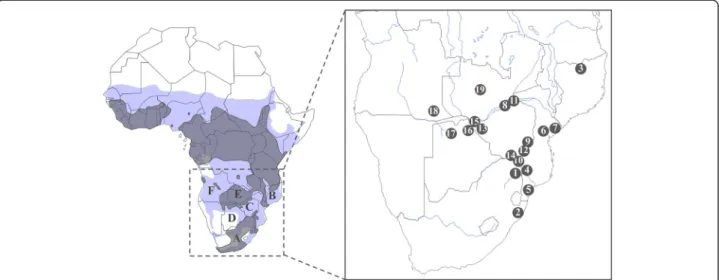
authorities in Bostwana, Mozambique, South Africa and Zimbabwe; Mario Melletti obtained the relevant permits to export samples from the wildlife manage-ment authorities of Zimbabwe and the University of Pretoria (South Africa) from the Hluhluwe-iMfolozi National Park. All partners obtained the ethical ap-proval from their institution for the sampling proced-ure. The animal sampling protocols did not induce pain or distress according to the Animal Care Resource Guide (USDA category C). To facilitate the procedure, sampling of peripheral tissue (i.e. ear) or hair required the capture of buffalo through chemical immobilisation. The animals were released under veterinary supervision in favourable conditions. A total of 264S. caffer caffer sam-ples were collected at 19 localities in 6 countries (Figure 1, Table 1). Hair and tissue samples were stored in 96% etha-nol. Genomic DNA was extracted from samples using the DNeasy Tissue Kit (QIAGEN Inc.) according to the manu-facturer’s protocol.

Microsatellite amplification and genotyping

The 264 samples used in this study were genotyped at 14 variable autosomal microsatellite loci (TGLA227, TGLA263, ETH225, ABS010, BM1824, ETH010, SPS115, INRA006, BM4028, INRA128, CSSM19, AGLA293, ILSTS026, DIK020- described by [39,40]). In addition, within this 264 samples set, all 86 males were also genotyped at three Y-chromosomal microsatellites (UMN1113, INRA189, UMN0304- described by [41]) (Additional file 1: Table S1). The three Y-chromosomal microsatellites were only used to reconstruct a minimum spanning network. Thirteen male samples failed to amplify at least at one

Figure 1 Map of Africa representing the 19 sampling localities of S. c. caffer analysed in this study. Grey shapes on the map represent the actual distribution of the African buffalo according to the IUCN Antelope Specialist Group, 2008. Blue shapes represent past distributions according to Furstenburg 1970–2008 (personal unpublished field notes). A. South Africa, B. Mozambique, C. Zimbabwe, D. Botswana, E. Zambia, F. Angola, 1. Kruger, 2. Hluhluwe-iMfolozi, 3. Niassa, 4. Limpopo, 5. Manguana, 6. Gorongosa, 7. Marromeu, 8. Nyakasanga, 9. Malilangwe, 10. Crooks Corner, 11. Mana Pools, 12. Gonarezhou, 13. Hwange, 14. Sengwe, 15. Victoria Falls, 16. Chobe, 17. Okavango Delta, 18. Angola, 19. Zambia.

Y-chromosomal microsatellite and were discarded for the minimum spanning network reconstruction (NMales= 73).

All those microsatellites were selected because they dis-played good quality and high polymorphic amplification. The forward primer of each locus was 5’-end labeled with a fluorescent dye. Four multiplex sets were elaborated

based on size limitations and amplification specificity: set 1 (TGLA227, TGLA263, ETH225, ABS010, UMN0304), set 2 (BM1824, ETH010, SPS115, INRA189), set 3 (INRA006, BM4028, INRA128, CSSM19), set 4 (AGLA293, ILSTS026, UMN113, DIK020). PCRs were carried out in 10 μl vol-umes containing between 0.1 and 0.2 μl of each 10 μM Table 1 Overview of the genetic parameters at each sampling locality

Country Sampling locality Fig 1 ID Area (km2) NTOT N Na Pa Ar HO (SD) H(SD)E Fis N cluster affiliation % C cluster affiliation % S cluster affiliation % South Africa Kruger 1 19,485 40 920 [32] 26 99 0 1.636 0.659

(0.204) 0.671 (0.203)

0.012 0 96.2 3.8 South Africa

Hluhluwe-iMfolozi 2 960 4 000 [21] 20 53 2 1.545 0.536 (0.250) 0.533 (0.226) 0.001 0 0 100 Mozambique Niassa 3 42,300 6 200 [33] 20 100 2 1.650 0.663 (0.180) 0.680 (0.226) −0.012 95 5 0 Mozambique Limpopo 4 11,230 200 [34] 6 57 0 1.653 0.617 (0.246) 0.653 (0.239) 0.069 0 100 0 Mozambique Manguana 5 - - 4 51 0 1.634 0.649 (0.282) 0.634 (0.234) −0.021 25 75 0 Mozambique Gorongosa 6 4000 360 (C. Pereira, Pers. Comm. - 2010) 7 61 0 1.671 0.626 (0.291) 0.671 (0.207) 0.091 0 100 0 Mozambique Marromeu 7 11,270 > 10 300 [35] 21 76 0 1.639 0.668 (0.228) 0.639 (0.225) −0.062 95.2 4.8 0

Zimbabwe Nyakasanga 8 1000 Unknown 2 36 1 1.806 0.542 (0.401)

0.597 (0.395)

0.063 100 0 0

Zimbabwe Malilangwe 9 405 Unknown 20 97 2 1.659 0.636 (0.225) 0.659 (0.244) 0.008 35 55 10 Zimbabwe Crooks corner 10 - Part of transfrontalier PA - 13 81 1 1.634 0.581 (0.205) 0.634 (0.236) 0.058 0 100 0

Zimbabwe Mana pools 11 6766 Unknown 10 90 1 1.700 0.641 (0.318) 0.700 (0.285) 0.120 60 40 0 Zimbabwe Gonarezhou 12 7110 2 742 [36] 42 102 1 1.636 0.601 (0.256) 0.636 (0.255) 0.029 11.9 81 7.1 Zimbabwe Hwange 13 14,651 Hwange

and adjacent area: 24 500 [37] 6 63 0 1.598 0.557 (0.295) 0.628 (0.298) 0.052 33.3 66.7 0 Zimbabwe Victoria falls 15 23 15 96 1 1.663 0.629

(0.307) 0.663 (0.261)

0.008 66.7 26.7 6.6

Zimbabwe Sengwe 14 - transnational corridor between Kruger and Gonarezhou - 8 73 0 1.646 0.571 (0.253) 0.646 (0.279) 0.076 0 75 25

Botswana Chobe 16 11,700 Northern Botswana: 39 580 [38] 22 95 1 1.641 0.612 (0.250) 0.637 (0.262) 0.067 77.3 22.7 0 Botswana Okavango delta 17 16,000 20 92 0 1.633 0.616 (0.254) 0.628 (0.257) −0.003 90 5 5

Angola Angola 18 No precise locality - 1 22 3 1.583 0.571 (0.514)

0.571 (0.514)

- - -

-Zambia Zambia 19 No precise locality - 1 24 0 1.667 0.714 (0.469)

0.714 (0.469)

- - -

-This summarises the sample origin (country and sampling locality), size of the sampling locality in square kilometres, estimated number of buffaloes by aerial counts (NTOT), sample size per sampling locality involved in the present study (N) and mean values for number of alleles (Na), private alleles (Pa), allelic richness (Ar), observed (HO) and unbiased expected heterozygosity (HE) (and their standard deviations SD) and inbreeding coefficient (Fis) across autosomal microsatellite

loci. The affiliation of each sampling locality to each cluster, expressed in percentage, is also given in the last three columns (C; Central cluster, N; Northern cluster, S; Southern cluster).

diluted primer (forward and reverse), 5μl Multiplex PCR Master Mix (QIAGEN) and 2.5 μl DNA. Amplifications were performed in thermal VWR Unocycler using an acti-vation step (94°C/15 min) followed by 30 cycles (denatur-ation at 94°C for 30 s, annealing at 57°C for 90 s, extension at 72°C for 60 s) and final extension step at 60°C for 30 min. PCR products were genotyped on a Applied Biosystems 3130XL Genetic Analyzer using 2μl of ampli-fied DNA, 12 μl of Hi-Di formamide and 0.4 μl of GeneScan-500 (LIZ) size standard (Applied Biosystem). Length variation determination was performed using GENEMAPPER 4.0 (Applied Biosystems).

Microsatellite analysis

Genetic diversity and differentiation

MICRO-CHECKER 2.2.3 [42] was used to estimate the proportion of null alleles (NA) at each locus, calculated for each cluster (defined by STRUCTURE- see below), as well as the stutter errors or short allele dominance. The genotypes were then corrected relative to the results obtained with MICRO-CHECKER 2.2.3. Tests for linkage disequilibrium between loci for each sampling locality (SL) (Table 1), and the data fit to the Hardy-Weinberg equilibrium (HWE) proportions for each locus separately and over all loci for each SL, were performed with GENEPOP ([43] accessible online at: http://gene-pop.curtin.edu.au/). For both analyses, the Markov chain method was used with 1000 dememorizations, 1000 batches and 1000 iterations per batch. Fisher’s method for combining independent test results across SL and loci was used to determine the statistical significance of the test results.

Genetic diversity was assessed by calculating the ex-pected (HE) and observed (HO) heterozygosities for each

SL using both ARLEQUIN version 3.1 [44] and FSTAT 2.9.3 [45]. The DEST estimator [46], as well as

conven-tional pairwiseFSTstatistics [47], were assessed using the

online SMOGD application (http://www.ngcrawford. com/django/jost/) with 1000 bootstrap replicates [48], and ARLEQUIN 3.1, respectively. This allowed us to as-sess differences in allelic diversity among clusters. DEST

appeared to be more accurate than GSTand its

deriva-tives [46] for highly polymorphic markers such as micro-satellites. FST was estimated for comparison with DEST,

but also because it has been suggested to be more appropriate when both the sample size and number of applied loci are relatively low [49]. The hierarchical dis-tribution of genetic variance among and within popula-tions, based on F-statistics, was assessed using an analysis of molecular variance (AMOVA) performed with ARLEQUIN 3.1. The populations for the AMOVA analysis were defined according to the clustering results obtained with STRUCTURE 2.3. Allelic richness (AR

-[50]) was calculated for each SL using the rarefaction

procedure implemented in FSTAT 2.9.3 [45], which also allowed estimation of the multi-locus FIS. The

signifi-cance level was sequentially Bonferroni-adjusted for re-peated tests [51].

A linear regression between patch areas (expressed as log km2) and different genetic indices of differentiation (mean pairwise DESTand mean pairwiseFST) and

diver-sity (allelic richness ARand expected heterozygosityHE)

for each SL were also performed to assess the effect of confinement within small enclosed protected areas (details for each SL are displayed in Table 1).

Population structure

Bayesian clustering of microsatellite genotypes was per-formed using STRUCTURE 2.3, pooling individuals to-gether independently of the spatial sampling, as described in the manual [52,53]. This software is imple-mented to cluster a sample set into a K number of groups so that each group is homogeneous. The number of clusters (K) was inferred by running 10 iterations for each K value from 1 to 20 using an admixture model with a burn-in of 1 × 105and MCMC repetition values of 1 × 106. As the STRUCTURE software does not pro-vide a statistical indication of the most likely K, results of the 10 iterations for each K value were summarized and averaged using CLUMPP 1.1.2 [54]. The K value that best fits the structure of the data set was revealed by the increasing likelihood of the data. It is chosen as the smallest value of K capturing the major structure in the data. The optimal number of clusters was then assessed based on correction as defined by Evanno [55]. Visual output of the STRUCTURE 2.3. analysis was gen-erated using DISTRUCT 1.1 [56]. Cluster membership of each sample was determined based on the average probability estimates provided by CLUMPP. The highest probability of each sample to belong to each cluster was used to determine its affiliation for the subsequent analyses. In the present study, the “cluster” term was at-tributed to define groups of individuals defined by STRUCTURE analysis, whereas “sampling locality” (SL) designates individuals sampled in the same protected area. Moreover, three male-specific non-recombining micro-satellites (UMN0304, UMN1113 and INRA189) located on the Y-chromosome were selected for complementary analyses. Haplogroups were defined as a combination of the haplotypes defined for each of the three Y-chromosomal microsatellites, as described in the study of van Hooftet al. [41], while taking all three loci {n1, n2, n3} into account. Haplotypes for each

microsat-ellite had to be defined because they could appear as multicopies on the Y-chromosome [41]. A minimum spanning network reconstruction was manually drawn by minimization of the number of mutations between haplotypes.

A factorial correspondence analysis (FCA), represent-ing the proximity between each individual genotype in a 2D plot was performed based on the microsatellite allele frequencies using R software version 2.15.2 (R Develop-ment Core Team 2008) and the ade-4 package [57] using the 'fuzzygenet' function. Recent demographic bottle-necks were further investigated with BOTTLENECK 1.2 [58]. This software computes the average heterozygosity, which is compared to the observed heterozygosity to de-termine if a locus expresses a heterozygosity excess/deficit, according to the strict Stepwise Mutation Model (SMM [59]). Estimations were based on 1000 replications. Demographic history

For all subsequent analyses, software were run on two dis-tinct microsatellite matrices: (i) a first one that included all individuals pooled together in each cluster determined by STRUCTURE 2.3, and (ii) a second matrix that only in-cluded individuals displaying a probability of belonging to each of the clusters over 0.9 (STRUCTURE 2.3). This measure was necessary to avoid bias associated with the high number of translocations that have taken place over the last decades in southern Africa (see Discussion).

The evolutionary history of S. c. caffer in southern Africa was inferred using coalescent-based DIYABC 1.0.4.45 beta software [60]. This program infers the popu-lation history by looking backwards in time to examine the genealogy of alleles until reaching the most recent common ancestor. The coalescent-based approximate Bayesian computation algorithm of DIYABC estimated the splitting time (in generation) as well as the effective population size of each tested cluster. Three clusters (or populations) were defined with STRUCTURE 2.3, with one almost exclusively composed of individuals from the Hluhluwe-iMfolozi PA. However, this last SL originated from an estimated population size of 75 individuals in 1929, after a population crash due to a rinderpest epi-demic that eradicated around 95% of the South African buffalo population [20]. Only the two other clusters were considered in this analysis in order to avoid bias associ-ated with a recent founder event and subsequent genetic drift.

Alternative biogeographic divergence scenarios were inferred and compared using the DIYABC software package. In-depth information about scenario building procedure and alternative competitive scenario represen-tations are available as additional file (Additional file 2: Figure S1A and S1B). Two runs were performed, a first one consisting of all scenarios (Additional file 2: Figure S1A and S1B), and a second one whereby only scenarios having the highest posterior probabilities were taken into consideration. The range and distribution of prior for parameters used to describe these scenarios (effective population size, time of splitting or merging events, and

admixture rates) are given as additional file (Additional file 3: Table S2). For the second run, 3,000,000 datasets were simulated for each scenario (Figure 2) by building a reference table from a specified set of prior parameter distributions. A principal component analysis (PCA-DIYABC, Additional file 4: Figure S2) was performed on the first 30,000 simulated datasets to check if the set of scenarios and the prior distributions of their pa-rameters were able to generate datasets similar to the observed dataset. A normalized Euclidean distance be-tween each simulated dataset of the reference table and the observed dataset was calculated to identify the most likely scenario. To estimate the relative pos-terior probability of each scenario, 1% of the closest simulated datasets was used in a logistic regression. The most likely scenario was the one with the highest posterior probability.

Similarly, an isolation by distance (IBD) analysis among and within the three clusters defined with STRUCTURE 2.3 [52] was performed with GENEPOP 4.1.2 [61]. TheDσ2estimates (i.e. product of population density and axial mean square parent-offspring distance as defined by [62]), were calculated according to b = 1/ (4π Dσ2_{) to estimate the signal strength. The value}

ob-tained (Dσ2_{) was inversely correlated with the IBD}

strength. The geographic distance was calculated using the logarithm of the Euclidean distance on GPS coordi-nates.ârstatistics were used to represent the genetic

dis-tance between pairs of individuals [61]. We tested the significance of the correlation using a Mantel test with 30,000 permutations [63].

Furthermore, MIGRATE 3.4.4 [64-66] was used on the three populations. This allowed us to estimate dif-ferent historical demographic events and genetic pa-rameters, including the effective population size, the extent to which the clusters interacted (i.e. (im)migra-tion rate (M)), and the confidence intervals. This ana-lysis was developed by measuring similarities among our three clusters based on optimized FST-based

mea-sures. This software employs a Metropolis-Hastings Markov chain Monte Carlo algorithm (MH) to search through genealogies, and a likelihood ratio test to ob-tain estimates of theta (Θ) and M. It assumes a con-stant Θ for each population but a variable Θ between them (pairwise migration rate estimates). MIGRATE 3.4.4 was used with default parameters, with the first five runs including FST- based statistics of Θ and M

involving 10 short chains with 10,000 sampled geneal-ogies and three long chains with 100,000 sampled ge-nealogies. A second analysis with five additional runs was performed with the parameter estimates of Θ and M from the previous run as starting values. Run con-vergence was checked by computing the MCMC autocorrelation, effective sample size and by visual

comparison of the consistency of the results of each of the independent analyses. The headcount of immi-grants per generation was calculated according to xNem =M*Θ, with x being the inheritance scalar, set

at 4 for diploid species, Ne the effective population

size, and m the mutation rate per generation and per locus. The effective population size was assessed as-suming a mean mutation rate within a range of 4.5*10−5 to 15*10−5 per generation.

Results

Population structure

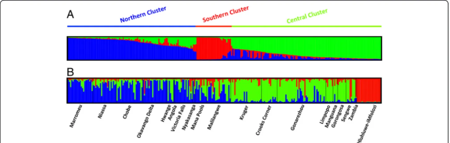
The STRUCTURE 2.3 software output was interpreted using the ΔK method, as described by Evanno [55]. The highestΔK was for K = 3 (Figure 3 and Additional file 5: Figure S3), suggesting the existence of three clusters in our dataset (ΔK = 262.2). These clusters were considered as different “populations” in the subsequent analyses. The proportion of each cluster within every sampled

Figure 2 Representation of three final competing scenarios tested with approximate Bayesian computation (ABC). This analysis was based on a matrix including individuals displaying a probability of belonging to one of the two clusters over 0.9 (STRUCTURE software). Ni

corresponds to effective population size of each cluster, and Ticorresponds to the time expressed in numbers of generations since divergence.

The following conditions were considered: T1< T2, T2< T3, with 0 being the sampling date. Abbreviations are as follows: C; Central cluster, N;

Northern cluster, PP; Posterior probability and their associated 95% confidence interval.

Figure 3 Clusters inferred with STRUCTURE software, after the Evanno correction (K = 3). The cluster membership of each sample is shown by the colour composition of the vertical lines, with the length of each colour being proportional to the estimated membership coefficient. The spatial representation is shown in Figure 4. A. Representation of the 3 clusters identified with STRUCTURE; B. Representation of the cluster membership of each sample within each sampling localities.

locality is represented in Figure 4. The first cluster –N-(in blue in Figure 4) mainly appeared in samples collected in the northern section of the study area (all samples of Nyakasanga and Mana Pools, a large part of the samples from Niassa, Marromeu, Victoria Falls, Okavango Delta and Chobe, as well as from Hwange, to a lesser extent). The second cluster –C- (in green on Figure 4) appears in the central section of the study area, and is represented in very high proportions in the sets of samples from Kruger, Sengwe, Manguana, Limpopo and Hwange. The third cluster –S- (in red on Figure 4) es-sentially includes samples from Hluhluwe-iMfolozi, al-though residual shared loci were observed at other sampling localities.

Note that most clusters appeared to be admixed (Figure 4). This could partially be due to translocation operations since quite a large number of buffaloes have been captured and translocated in recent years. For ex-ample, the original buffalo population of Gorongosa (number 6 on Figure 4) was nearly extinct and recently reinforced with 186 buffaloes translocated from Kruger and adjacent Limpopo PAs (2006–2011; C. Lopes Pereira, pers. com.). In the present study, all samples

from Gorongosa were reintroduced buffaloes from those latter two localities (C. Lopes Pereira, pers. comm.).

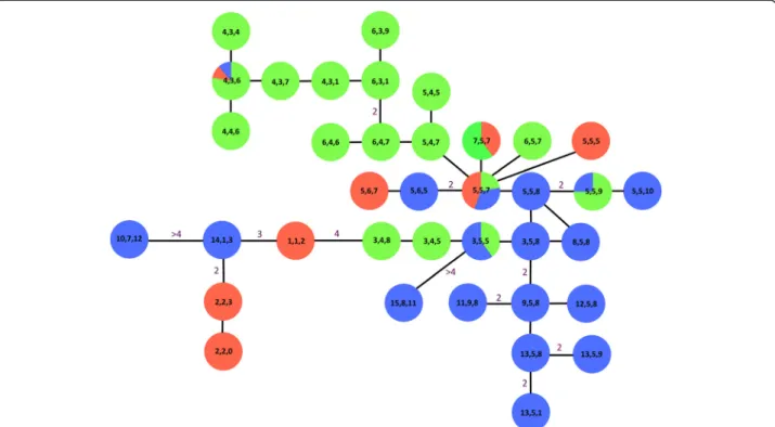
A similar general genetic pattern can be noted on the Y-chromosomal microsatellite minimum spanning net-work reconstruction (Figure 5). Seventy-three male spec-imens were genotyped with the Y chromosomal microsatellites. Twenty-six haplogroups were observed in southern Africa, pooled with the haplogroups identi-fied by van Hooftet al. [41], with each haplogroup being a unique combination of the haplotypes defined for each of the three Y-chromosomal microsatellites, i.e. {nUMN1113 haplotype, nUMN0304 haplotype, n INRA189 haplotype}

(Table 2). More precisely, we respectively observed 15, 9, and 12 haplotypes at the UMN1113, UMN0304 and INRA189 loci. The detailed polymorphic loci of each of these microsatellites as well as their frequencies are re-ported in Table 2. Haplogroups {5, 5, 7} and {2, 2, 3} were present at the highest frequencies, namely 0.123 and 0.110, respectively, followed by {4, 4, 6} with 0.082, exclu-sively from Sengwe, and {3, 5, 5} with 0.069 found in Chobe, Nyakasanga, Malilangwe and Mana Pools. The other haplogroups did not overstep a frequency of 0.055. Moreover, only haplogroups {5, 5, 7} and {4, 3, 6} were

Figure 4 Geographical representation of the three clusters assessed with STRUCTURE software (for SLs with Nind> 3). Angola and

Zambia are not represented due to the low sample sizes from those areas. Blue corresponds to the Northern cluster (N), green to the Central cluster (C) and red to the Southern cluster (S). The sampling localities are also given: 1. Kruger, 2. Hluhluwe-iMfolozi, 3. Niassa, 4. Limpopo, 5. Manguana, 6. Gorongosa, 7. Marromeu, 8. Nyakasanga, 9. Malilangwe, 10. Crooks Corner, 11. Mana Pools, 12. Gonarezhou, 13. Hwange, 14. Sengwe, 15. Victoria Falls, 16. Chobe, 17. Okavango Delta.

observed in the three clusters. Figure 5 shows moderate structuring of the two main clusters (i.e. the Northern (blue) and the Central (green) clusters, identified by STRUCTURE 2.3). This was not the case for the more dis-parate Southern cluster (red).

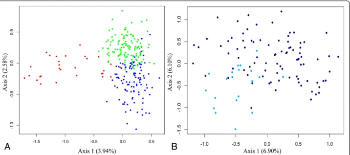
Finally, the three clusters identified by STRUCTURE 2.3 appeared to be relatively well defined, with the Southern cluster being more clearly separated from the two others based on visual assessment of the FCA plot (Figure 6A.). Furthermore, within the Northern cluster, a very smooth separation appeared between the Marromeu SL compared to all other SLs included in this cluster (Figure 6B).

Genetic diversity

As highlighted in previous studies using the same micro-satellites in different geographical areas [39-41], all microsatellites were detected as being polymorphic in each of the SL of the southern African sub-region. The number of alleles per microsatellite ranged from 2 to a maximum of 23 (Additional file 1: Table S1, Additional file 6: Table S3). The mean number of alleles across loci ranged from 6.3 in the Southern cluster to 9.5 in the Northern cluster. A significant presence of null alleles

was detected for microsatellites BM1824 and INRA006 in the Northern cluster, and for TGLA227, BM1824 and AGLA293 in the Central cluster. They were corrected as suggested in the MICRO-CHECKER 2.2.3 user manual. A Hardy-Weinberg exact test performed on each SL at each loci showed no deviation from the expected frequencies after Bonferroni’s correction. One pair of loci (SPS115 and DIK020) was found to show significant linkage disequilibrium in two populations (Northern and Central clusters). No single microsatellite marker exhibited an especially high number of private alleles (Additional file 1: Table S1).

Overall, the genetic variation level was high in all clus-ters. Inbreeding coefficients (FIS) were low to moderate

but significant for all three clusters (Table 3). This index showed more variation when calculated for each SL sep-arately, with a high FIS value (0.12) for Mana Pools

(Table 1). The microsatellite genetic diversity analysis showed that pairwise differences andFSTwere significant

between all three clusters (Table 4), which was not al-ways the case between animals from different SLs within each of the clusters (Table 5). Similar pattern were ob-served regarding pairwise FST and DEST values among

SLs and clusters: lower genetic differentiation among the

Figure 5 Minimum spanning network reconstruction based only on the three Y chromosomal microsatellites. It was manually drawn by minimization of the number of mutations between haplotypes. The three numbers in boxes refer to the different haplotypes at microsatellites UMN0304, UMN113, and INRA189, respectively, as described in van Hooft et al. [41]. Our dataset was standardized and pooled with the data of van Hooft et al. [41] that were absent from our sampling, i.e. (4, 3, 4), (4, 3, 7), (4, 3, 1), (6, 3, 1), (6, 3, 9), (5, 4, 5), (5, 4, 7), (5, 6, 7), (5, 5, 5), (2, 2, 0) and (3, 4, 8) from the Kruger and Hluhluwe-iMfolozi PAs. Numbers on the branches indicate the minimum number of mutations (when absent, only one mutation was observed between haplogroups). Box colours refer to the three clusters identified with the autosomal microsatellites using STRUCTURE software. The three most frequent haplogroups were (2, 2, 3), (5, 5, 7) and (4, 3, 6) (see Table 2).

Central SLs and low/moderate differentiation among the Northern SLs (Table 5). Moreover, we found higher gen-etic differentiation between the Northern/Central clus-ters and the Southern cluster (FST and DEST -Tables 4

and 6). The mean observed heterozygosity ranged from 0.56 to 0.66, and was within the range of the main ex-pected heterozygosity reported in Table 3. Allelic rich-ness reached up to 7.8 in the Northern cluster (Table 3). The average number of alleles, average genetic diversity over loci, allelic richness, and heterozygosity were simi-lar in the Northern and Central clusters. Interestingly, the results of the Wilcoxon test under a stepwise muta-tion model performed using the BOTTLENECK 1.2 soft-ware package indicated that the Southern and Central clusters had undergone a recent bottleneck (probability

of 0.007 and 0.032, respectively), whereas the Northern cluster did not (probability of 0.191).

Demographic history

The DIYABC 1.0.4.45 beta software package was used to determine which historical demographic scenario could best explain the observed microsatellite polymorphism. The approximate Bayesian computation approach was used on 16 distinct demographic scenarios (Additional file 2: Figure S1A and S1B), followed by a second ana-lysis with only three demographic scenarios that pre-sented the highest posterior probabilities (PP) in the first run [67,68]. The last three competing scenarios included in the second run revealed a similar general evolutive demographic pattern (Figure 2), namely a binary split Table 2 Haplotype designation, haplogroup determination and their frequencies for the three Y-chromosomal micro-satellite loci (UMN0304, UMN1113 and INRA189, NMales= 73)

UMN0304 alleles combination UMN0304 haplotype designation UMN113 allele combination UMN113 haplotype designation INRA189 allele combination INRA189 haplotype designation Haplo-group Freq 215-225 1 131 1 148-153-158-166 2 {1,1,2} 0,014 217-227 2 133 2 148-153-158-164 3 {2,2,3} 0,110 205-215-225 3 131-157 4 148-162 5 {3,4,5} 0,014 205-215-225 3 131-155 5 148-158 5 {3,5,5} 0,069 205-215-225 3 131-155 5 148-158 8 {3,5,8} 0,027 205-217 4 131-159 3 160 6 {4,3,6} 0,123 205-217 4 131-157 4 160 6 {4,4,6} 0,082 205-215-223 5 131-155 5 148-160 7 {5,5,7} 0,123 205-215-223 5 131-155 5 148-158 8 {5,5,8} 0,014 205-215-223 5 131-155 5 151-156 9 {5,5,9} 0,055 205-215-223 5 131-147-155 6 148-158 5 {5,6,5} 0,027 205-217-223 6 131-157 4 160 6 {6,4,6} 0,014 205-217-223 6 131-157 4 148-160 7 {6,4,7} 0,027 205-217-223 6 131-155 5 148-160 7 {6,5,7} 0,014 215-223 7 131-155 5 148-160 7 {7,5,7} 0,041 205-215 8 131-155 5 148-158 8 {8,5,8} 0,014 205-217-227 9 131-155 5 148-158 8 {9,5,8} 0,014 217-223 10 131-133-147-155 7 137-148-158-162 12 {10,7,12} 0,014 205-215-227 11 133-155 9 148-158 8 {11,9,8} 0,055 205-221-227 12 131-155 5 148-158 8 {12,5,8} 0,027 205-213-227 13 131-155 5 151-156 9 {13,5,9} 0,014 205-213-227 13 131-155 5 151-160 1 {13,5,1} 0,014 205-213-227 13 131-155 5 148-158 8 {13,5,8} 0,014 217-225-227 14 131 1 148-153-158-164 3 {14,1,3} 0,027 213-225 15 133-147-155 8 151-153-162 11 {15,8,11} 0,014 205-215-223 5 131-155 5 148-151 10 {5,5,10} 0,041

Each haplotype was attributed a number to designate the combination of alleles for each of the three loci because they can appear as multicopies on the Y-chromosome. The haplogroup is thus defined as the combination of the haplotypes, written as {nUMN1113 haplotype, nUMN0304 haplotype, nINRA189 haplotype}, where n UMN1113 haplotype= 1,…,15, nUMN0304 haplotype= 1,…,9, and nINRA189 haplotype= 1,…,12.

without admixture events. After polychotomous logistic regression on the 1% closest simulated datasets to the observed one, the most likely scenario according to DIYABC 1.0.4.45 beta was scenario 3, as represented in Figure 2, with a PP of 0.402 and a confidence interval (95 CI) of 0.397–0.408. The PP of scenario 3 did not overlap with the two alternative scenarios. When com-paring the posterior distribution of parameters of those three competitive scenarios, the differentiation time at time T1 and the effective population size estimates

(N1 and N2) were all within same order of magnitude.

The median (95% CI) of the estimated time since diver-gence (T1) between the N and C clusters was evaluated

at about 1200 generations earlier (Figure 2). Assuming a generation time of 5–7 years, divergence time corre-sponds to the Holocene epoch (T1: 6000 to 8400 years

ago). The effective population size estimates for the C and N clusters reached a mean of 4700 and 6400 indi-viduals, respectively (Figure 2). The effective population sizes assessed with MIGRATE 3.4.4, assuming a mean mutation rate of 4.5*10−5to 15*10−5per generation, was estimated between 7000 to 25,000 for the Northern clus-ter, 600 to 2000 for the Southern cluster and 3000 to 10,000 for the Central cluster. In agreement with the

summary statistics of DIYABC 1.0.4.45 beta and the pre-viously estimated summary statistics described hereafter, there were no obvious differences between estimates of heterozygosity, genetic diversity andFST.

Migration rate could not be assessed with the IM soft-ware (for more information- see Additional file 7: IM), probably linked to the very high variation percentage within clusters (87.40%) as compared to the variation among them (12.60%) (AMOVA). MIGRATE 3.4.4 was used for this purpose, immigration rate per generation being calculated according to Nem = (Mi →j*Θj)/4, with

ΘS= 0.38,ΘN= 4.40,ΘC= 1.81 andMC→S= 4.17,MS→N=

0.84, MC→N= 2.56, MS→C= 1.06, MN→C= 5.01, MN→S=

1.67. The effective number of immigrants per gener-ation between clusters was low, from less than one mi-grant per generation (each 5–7 years) coming from the Southern towards the Central/Northern clusters, and vice versa (NmN→S= 0.16, NmS→C= 0.48, NmC→S= 0.40,

NmS→N= 0.92), to approximately two migrants between

the Central and Northern clusters (NmN→C= 2.27 and

NmC→N= 2.81). The results between the two runs on

the separate microsatellite matrices were similar. Finally, an IBD analysis was performed on the two microsatellite matrices to test whether the geographic

Figure 6 Plot of the factorial correspondence analysis (FCA). A.: Global FCA including the three clusters. Red: Southern cluster, Green: Central Cluster, Blue: Northern Cluster. B.: FCA on the Northern cluster. Turquoise: Marromeu samples, Dark blue: other populations included in the Northern cluster.

Table 3 Overview of the genetic parameters at each cluster

Cluster N NMales NFemales Na(SD) Pa Ar HO(SD) HE(SD) FIS Average genetic diversity over loci (SD) Northern 108 35 73 9.500 (5.360) 13 7.834 0.656 (0.242) 0.668 (0.264) 0.016 0.608 (0.319)

Central 125 35 90 9.143 (5.614) 8 7.657 0.635 (0.213) 0.657 (0.224) 0.033 0.601 (0.318) Southern 31 16 15 6.286 (3.518) 2 6.160 0.556 (0.208) 0.591 (0.205) 0.062 0.573 (0.303)

N: Number of samples, Na: Mean number of alleles, Pa: Private alleles, Ar: Allelic richness, HO: Observed heterozygosity, HE: Expected heterozygosity, FIS: Inbreeding

distance could explain the low number of migrants. Both runs indicated an absence of isolation by distance among clusters but a significant signal within the Northern and Central clusters (Dσ2

Central cluster= 9.95,Dσ2Northern clus-ter= 2.69). The analysis was not performed on the third

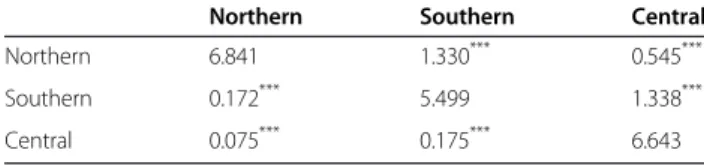
cluster because all samples in this cluster originated Table 4 Differentiation results obtained with ARLEQUIN

software (calculated on the matrix including individuals displaying a probability of belonging to one of the three clusters over 0.9 (STRUCTURE software))

Northern Southern Central Northern 6.841 1.330*** _0.545*** Southern 0.172*** _{5.499 1.338}*** Central 0.075*** _0.175*** _6.643

Below diagonal, FSTvalue- Diagonal elements, average number of pairwise

differences within population (PiX)- Above diagonal, corrected average pairwise difference (PiXY-(PiX + PiY)/2).***

indicates P < 0.0005.

Table 5F_ST(Below diagonal- ARLEQUIN software) andD_EST(Above diagonal- SMOGD software) for the 16 geographical populations 1 (N) 2 (N) 3 (C) 4 (S) 5 (C/N) 6 (C) 7 (N) 8 (C) 9 (C) 10 (N) 11 (C) 12 (C) 13 (C) 14 (C) 15 (N) 16 (N) 1 (N) / 0.056 0.079 0.247 0.043 0.066 0.093 0.084 0.063 0.001 0.084 0.091 0.018 0.051 0.057 0.074 2 (N) 0.033 *** / 0.058 0.225 0.001 0.076 0.001 0.007 0.075 0.019 0.065 0.078 0.009 0.086 0.090 0.001 3 (C) 0.041 *** 0.036*** / 0.213 0.001 <_−0.0001 0.037 0.004 −0.010 0.007 0.015 <0.0001 <_−0.0001 0.0002 0.105 0.060 4 (S) 0.163 *** 0.167*** 0.141*** / 0.236 0.235 0.245 0.177 0.234 0.293 0.244 0.141 0.142 0.148 0.290 0.242 5 (C/ N) 0.037 * −0.007ns 0.026 * 0.196 *** / 0.002 −0.0001 0.002 0.007 0.0001 0.016 0.024 <0.0001 0.037 0.064 0.009 6 (C) 0.042 * 0.056*** 0.010ns 0.181*** 0.056*** / 0.012 0.006 0.003 0.023 0.019 <0.0001 <0.0001 0.011 0.087 0.034 7 (N) 0.045 *** 0.006ns 0.033*** 0.157*** 0.004ns ***0.062 / 0.019 0.050 0.006 0.041 0.081 0.008 0.066 0.083 0.005 8 (C) 0.044 *** 0.020*** 0.014 * _0.130 *** 0.016ns 0.034 * _0.022* _{/ 0.012 0.018 0.017 0.008 <} −0.0001 0.021 0.118 0.012 9 (C) 0.049 *** 0.051*** −0.008ns 0.175*** 0.056*** 0.024 ns 0.059 *** 0.025 * / 0.003 0.005 −0.007 < −0.0001 0.001 0.116 0.062 10 (N) 0.016 * 0.029*** 0.021 * _0.163 *** 0.010ns 0.032 * _0.021ns _0.027* _0.035* _{/ 0.021 0.002 0.010 0.013 0.081 0.009} 11 (C) 0.037 *** 0.030*** 0.008 * 0.154 *** 0.031 * 0.013ns 0.031 *** 0.012 * 0.013 ns 0.025* / 0.005 −0.008 0.005 0.111 0.047 12 (C) 0.046 * 0.060*** 0.002ns 0.128*** 0.053ns 0.005 ns _0.060* _0.023 ns 0.002ns 0.016ns 0.026 * _{/ 0.003 0.020 0.112 0.046} 13 (C) 0.037 * 0.030ns −0.015ns 0.139*** 0.029ns 0.007 ns 0.029ns −0.005 ns −0.009ns 0.029ns −0.013ns 0.011 ns / −0.0002 0.048 0.025 14 (C) 0.020 * 0.036*** −0.010ns 0.133*** 0.043ns 0.030 ns _0.043* _0.018* _−0.010 ns 0.030ns 0.010ns 0.026 ns _−0.012 ns / 0.109 0.065 15 (N) 0.034 *** 0.059*** 0.064*** 0.195*** 0.055*** 0.067*** ***0.055 0.064*** 0.081*** 0.050*** 0.063*** 0.073*** 0.051 * 0.064 *** / 0.082 16 (N) 0.032 *** −0.001ns 0.045*** 0.166*** −0.003ns 0.059*** 0.008 ns _0.012* _0.068 *** 0.022*** 0.036*** 0.060*** 0.037 * _0.047 *** 0.058*** /

These estimators were only computed where more than 5 samples were available. 1: Niassa, 2: Chobe, 3: Kruger, 4: Hluhluwe-iMfolozi (bold), 5: Hwange, 6: Sengwe, 7: Victoria Falls, 8: Malilangwe, 9: Crooks Corner, 10: Mana Pools, 11: Gonarezhou, 12: Limpopo, 13: Manguana, 14: Gorongosa, 15: Marromeu, 16: Okanvango Delta. Cluster affiliation of each sampling locality is also indicated in the table as follow: (N) for the Northern cluster, (C) for the Central cluster and (S) for the Southern cluster. Here, one SL is considered to belong to one cluster if there are more than 50% of SL’s individuals that belongs to this cluster.*

indicates P < 0.05,**

indicates P < 0.005,***

indicates P < 0.0005;nsindicates non-significant.

Table 6 Harmonic mean ofD_ESTacross loci between each of the three clusters (SMOGD software)

Northern Southern Central

Northern 0.281 0.137

Southern 0.276

Central

This computation was performed on the matrix, including individuals displaying a probability of belonging to one of the three clusters over 0.9 (STRUCTURE software).

from a single protected area, i.e. Hluhluwe-iMfolozi. The signal in the Central cluster was not strong, as indicated by the relatively high Dσ2value and by the slight slope of the regression of pairwise genetic statistics against the log distance. The slight regression slope indicated that the genetic distance between pairs of individuals was weakly correlated with the geographic distance between them. The signal was stronger in the Northern cluster. The absence of significant signal between the three clus-ters showed that the cluster generation was not driven by the geographic distance. Concerning the linear re-gression performed between the log habitat area and the different genetic differentiation indices and diversities for each SL, the R2(coefficients of determination) were close to 0. This indicated an absence of any linear rela-tionship between the log habitat areas and the different genetic indices (AR: R2= 0.03, MeanHE: R2= 0.05, Mean

pairwise DEST: R2= 0.04, Mean pairwise FST: R2= 0.05).

Graphic representations are available as supplementary information (Additional file 8: Figure S4).

Discussion

The present study provides new insight into the current genetic structure of buffalo populations in southern Africa, indicating the existence of three genetically and geographically distinct populations, or so-called meta-populations (Figure 4). The sampling covered a large part of the current distribution area of the southern African buffalo, thus ensuring robust analytical findings. We demonstrated that the three-cluster structuring did not result from isolation by geographical distance (IBD), but probably from other human and environmental fac-tors. We further discuss the impact of translocations on the genetic structure of southern African buffalo popula-tions, as well as the observed genetic diversities within and between each of the clusters/sampling locality (SL), from a wildlife conservation management standpoint. Demographic history of the Northern (N) and the Central (C) clusters

The time of splitting of the N and the C clusters was dated at about 6000 to 8400 years ago. This splitting time may be underestimated, given that the DIYABC al-gorithm assumes no migration between the scenario events [60]. The differentiation time may thus be an underestimation of the real splitting time. Nevertheless, our results are well corroborated by the findings of a previous study conducted by Helleret al. [31]. These au-thors compared Bayesian skyline plots of African buffalo samples from three localities (Zimbabwe/Bostwana, Ethopia and Kenya). A moderate and then accelerating buffalo population decline was highlighted over the course of the Holocene [31]. This decline suggests a major ecological transition between the Palaeolithic,

during which the buffalo population expanded, and the Neolithic, during which the buffalo population declined [31]. This was probably induced by two concomitant causal factors, i.e. climatic changes and explosive human population growth [31].

In the first case, climatic changes were proposed to have strongly impacted buffalo population dynamics. The Holocene was marked by rapid climate changes— from moist (African humid period), during which forests and woodlands expanded [69-71], towards increasingly drier conditions around 4000–6000 YBP, concomitantly with the buffalo population decline [31]. This consider-able and quite rapid climatic shift likely occurred on a large spatial scale, as declines in the African buffalo ef-fective population size were recorded in several African regions (East and South Africa) [31,72]. Climate change in the Holocene was likely severe enough to have con-siderably impacted the African buffalo [73], leading to population fragmentation.

In addition to the climate hypothesis, human popula-tions likely had an impact on the buffalo population fragmentation process. Indeed, according to Helleret al. [31], during the human Neolithic revolution, sub-Saharan human populations started to increase while, in-versely, the African Cape buffalo population started to significantly decrease. This human impact would have been enhanced around 2000 years ago [74]. Around that time, the first southern African states were established by prosperous cattle herding people who adopted crop farming. Cattle husbandry led to the development of complex societal and political systems [74-78]. By 1500 A.D., most of southern Africa was governed by so-cieties managing large domestic livestock herds (cattle, goat and sheep). Cattle populations increased rapidly fol-lowing the Neolithic revolution [72]. In this setting, it is likely that the southern African buffalo population pro-gressively suffered from competition with livestock for food resources and that significant discontinuities ap-peared in its initial distribution range. Moreover, it is also possible that aridification events of the Holocene drove humans and wildlife into closer contact around water resources, thus increasing ecological competition. Direct buffalo hunting, as a food supply and/or to re-duce competition with domestic livestock species, was likely another important factor.

The divergence between the N and C buffalo clusters could be explained by this break of continuity in the landscape matrix due to both aridification and progres-sive human/cattle population growth, and/or by poten-tial overhunting. At the regional level, the combined effects of rapidly expanding human activities and sudden climatic changes may have been primary forces that frag-mented a previously panmictic population and shaped the current genetic structure of African buffalo. In addition, N

and C clusters are hypothetised to share a common ances-tral population. The Y-chromosomal minimum spanning reconstruction identified a haplogroup, namely {5, 5, 7}, that was present in the three clusters and occurred in a central position, while displaying the highest frequencies of appearance (0.123). Its presence in all clusters could support our assumption of a common ancestral panmictic buffalo population that recently experienced fragmenta-tion. The isolation process persisted and amplified during the 20th century due to human and cattle population growth. A good example is central Zimbabwe, a plateau that offers excellent grazing between the Zambezi and Limpopo rivers. In this area, wild herbivores, including buffalo, are generally considered as disease reservoirs and were thus controlled or even eradicated over the last cen-tury to protect cattle on commercial farms.

A third potential explanatory factor of the isolation of N and C clusters concerns the spatial arrangement of the water system. Indeed, the African buffalo is a highly water dependent species and the large-scale distribution and regime of rivers may well explain the observed gen-etic structure. This seems possible since the ranges of N and C clusters roughly span the Zambezi and the Limpopo river basins, as well as Rovuma, Pungoe, Save and other river basins. Colonisation of southern Africa by buffalo from an eastern core (Uganda [17]) may have followed the primary river networks, thus leading to the emergence of two different genetic clusters. This hy-pothesis is not unlikely, but our recent study based on mtDNA [17] dated the buffalo colonisation of southern Africa at around 44,000 and 66,000 years ago. This pre-cedes the microsatellite-estimated splitting time between the N and C clusters by several tens of thousands of years. The hypothesis of a population fragmentation as-sociated with the rapid human demographic expansion and climatic changes a few thousands years ago there-fore seems much more likely.

Impact of translocations on the genetic structure of N and C clusters

Within the three identified clusters, discrepancies be-tween the genetic affiliation of some individuals and their geographical origins were observed (Figures 4 and 5). Natural migration and/or translocation of individuals could both be responsible for buffalo genetic patterns ob-served in southern Africa. As already mentioned, African buffalo is known to have a good dispersal capacity, as demonstrated in previous studies [13,15,24-26]. Never-theless, the immigration rates per generation between our three clusters appeared to be low, reaching a max-imum of two individuals per generation. Moreover, since a disease-free zone for commercial cattle farming was set up in central Zimbabwe, natural buffalo migration between northern and southern Zimbabwe is very

limited. Buffalo now still seem to migrate in smaller numbers across areas with fairly substantial human set-tlements, e.g. along rivers, but the reduced connectivity between the protected areas seems to affect its dispersal.

Translocations over the last century seem to best ex-plain the discrepancies observed in the identified genetic pattern highlighted in this study. In fact, records indicate that buffaloes from Malilangwe (C cluster) were pri-marly, but not exclusively, stocked with buffaloes from Hwange (N cluster) (C. Foggin, pers. comm.). Moreover, individuals from three different localities of the N cluster (Hwange, Chizarira and Charara) were moved to Gonar-ezhou (C cluster) (C. Foggin, pers. comm.). Save Valley, Bubye Valley and Nuanetsi buffalo populations, all lo-cated near Gonarezhou and Malilangwe (C cluster), were restocked from Hwange (N cluster—C. Foggin, pers. comm.) (Figure 7). Consequently, translocations seem to be the most plausible explanation for the lowerDEST

es-timates obtained between Malilangwe (C cluster) and Hwange/Victoria Falls/Chobe/Mana Pools complex (N cluster). In addition, translocation would also explain the very low DEST values between Hwange (N cluster)

and all C sampled localities, except for Gorongosa and Limpopo. Buffalo from Hwange, Lusulu (south of Chizarira) and Matusadona were selected to form herds free of foot-and-mouth disease, which is transmissible to cattle. These buffalo were then bred and subsequently transferred to many regions of Zimbabwe, including com-mercial wildlife properties adjacent to PAs (protected areas) within this country (C. Foggin, pers. comm.) [79].

Figure 7 Representation of known translocation events between Northern and Central protected areas of Zimbabwe. 1. Hwange, 2. Gonarezhou, 3. Malilangwe, 4. Save Valley, 5. Bubye Valley, 6. Nuanetsi, 7. Chizarira, 8. Charara. Blue: Northern cluster, Green: Central cluster.

The present study revealed a marked impact of transloca-tions on the regional genetic structure of the studied spe-cies. At a larger scale, the present findings highlighted the issue and impacts of translocations regarding species con-servation management. For endangered species, transloca-tion is often considered essential to restore genetic diversity of highly isolated populations threatened with ex-tinction and in areas where the species is extinct [6]. Nevertheless, for least vulnerable species such as the Afri-can buffalo (Least Concern- IUCN v.2013.2, downloaded on 8 December 2013), greater consideration should be given to cluster affiliations when planning translocations, if the relevant information is available. Failure to do so could interfere with local adaptations to specific environ-mental conditions. Not taking in consideration contem-porary micro-evolutionary change, often associated to human activities (ex. habitat fragmentation), may lead to ineffective or even detrimental management practices [80]. This consideration relates to the choice of the most appropriate options for improving the conservation man-agement of species populations regarding their environ-mental, behavioural and genetic specificities, as well as their conservation status (http://www.iucnredlist.org/). The ecological and evolutionary consequences of resource management decisions are further discussed in the review of Ashleyet al. [80], advocating evolutionary enlightened management.

The unique history of Hluhluwe-iMfolozi buffaloes (Southern cluster)

Hluhluwe-iMfolozi is a unique protected area as it has been completely isolated for about 100 years. Only 75 individuals were reported in this region in 1929, and this population may have been reduced partly as a result of the Nagana campaigns against the disease carrying tsetse fly (1919–1950) [20]. The current population (N = ± 4000 [21]) directly stems from these survivors, which could explain the recent bottleneck signal observed. Our genetic results support this isolation and population de-crease event. Indeed, the pairwise FSTand DEST indices

between the Southern cluster and the two other clusters had high values (more than twofold higher than between the N and C clusters), suggesting substantial isolation of the Southern cluster.

Nevertheless, and surprisingly, the Hluhluwe-iMfolozi buffalo population still harbours high estimated allelic richness, heterozygosity and genetic diversity. Note, however, that all of those estimates were lower as com-pared to those of the two other clusters, withFISvalues

two- and fourfold higher than for the C and the N clus-ters, respectively. The gene flow disruption due to a re-cent isolation (±17 generations) was likely responsible for the observed genetic erosion, with signs of inbreed-ing depression (FIS). In this setting, future increases in

genetic drift within the S population will probably lead to a more pronounced loss of genetic diversity as compared to the current situation, although faintly detectable by now. O’Ryan [20] similarly concluded that the Kruger population has retained most of its original variants present 100 years ago, in contrast to the Hluhluwe-iMfolozi, Addo and St Lucia populations which lost their variants through genetic drift. This trend is particularly clear when con-sidering the number of private alleles. Unique allele vari-ants were lowest in the S cluster (Pa= 2), while eight were

noted in the C cluster. The high genetic variation that is still being recorded may be explained by a his-torically large population size, with current buffalo popu-lation sizes still above the critical threshold (as discussed hereafter).

Within-cluster genetic diversity, differentiation and bottleneck signals

The N cluster had the highest mean number of alleles, private alleles (Pa= 13), heterozygosity and genetic

diver-sity estimates, while displaying the lowest inbreeding co-efficient. This may have been the result of a wider geographical distribution and higher population size esti-mates compared to the two other clusters (see next sec-tion). Moreover, in contrast with the two other clusters, the N cluster did not display any recent bottleneck sig-nal. The C cluster (which includes the Kruger and surrounding protected areas) is characterised by a sig-nificant signal of recent bottleneck. Buffaloes in the Kruger area were highly affected by rinderpest during the last decade of the 19thcentury, with a high mortality rate and a small number of survivors reported in 1902 [81]. The recent bottleneck signal may thus be associ-ated with this rinderpest outbreak. However, apart from the study of Helleret al. [31] which highlighted a bottle-neck signal caused by the rinderpest epidemic in the late 19th century, all other studies conducted on that topic demonstrated that the outbreak did not seem to impact the genetic variability of this population [14,20,82,83]. As previously proposed by van Hooft et al. [15], the ab-sence of genetic erosion also observed within our study could be explained by high gene flow between the C sampled localities, thus re-establishing the lost genetic variability. This assumption is supported by observed lowFSTandDESTvalues for the pairwise sampling

local-ities of the C cluster (Table 5), indicating high dispersal events between them. The high genetic variability in the C cluster is commonly recognised as being the result of two different features: (i) a very high ancestral popula-tion size [13,20], and (ii) a capacity to maintain a non-critical population size through a relatively high rate of increase [21] and a good dispersal ability [20,22,26,30,84]. This is not unlikely as the buffalo is vagile, with bachelor bulls readily travelling large distances between herds, with

entire herds sometimes moving and settling away from their initial ranges [25]. Groups of young females (less than 3 years-old) are often reported to escape through the Kruger fence into communal areas (R. Bengis, pers. comm.). This dispersive behavior may have helped the Southern African Cape buffalo population to recover its population size within 20–30 years after the rinderpest outbreaks [13,15,29,84]. Recolonization of the initial range from neighbouring protected areas, as also proposed by van Hooftet al. [15] regarding the Kruger PA, is the most plausible explanation for the high genetic diversity ob-served within the different sampling localities of the C cluster [15,85].

Within each of the N and C clusters, the SL showed a low level of genetic differentiation and high heterozygos-ity, comparable to the values obtained in previous stud-ies on the African buffalo. This extent of genetic diversity in African buffalo is particularly high as com-pared to estimates in other large African savanna ungu-lates [13,15,22]. At the SL scale, theDESTand traditional

pairwise FST statistical findings both lead to the same

conclusion. Almost allDESTbetween sampling sites were

extremely low within the C and N clusters (mean 0.007 and 0.022, respectively). This suggests the possibility of high gene flow within each of these clusters, as proposed hereafter. Nevertheless, in the N cluster, the mean DEST

were sixfold higher than in the C cluster, which may be partly explained by the higher DESTbetween Niassa and

all the other sampling sites (mean 0.050). This may be attributed to the geographical distance separating Niassa from all other sampling localities, as indicated by the significant IBD.

Interestingly, another complementary explanation may be linked to the very highDESTvalues of the Marromeu

complex, i.e. a network of protected areas (National Re-serve and Hunting Areas) included within the N cluster, as compared to the other SLs of the N cluster (mean DEST= 0.076) but also to SLs of the two other clusters

(mean DEST= 0.100). The Marromeu complex hosts a

high number of buffaloes (>10,300 individuals [35]) that have been relatively isolated for several centuries within a particular biotope, i.e. swamps in the Zambezi delta re-gion (C. Lopes Pereira, pers. comm.). When translo-cated, their adaptation to the typical habitats of surrounding buffalo populations (Miombo ecosystem) is very slow and lengthy (C. Lopes Pereira, pers. comm.) [80]. These animals thus appear to be adapted to flood-plains. Moreover, in 1996, the Marromeu buffalo popula-tion size was estimated to be about 2500 individuals [35], indicating that this population increased fourfold between then to now. While significant genetic drift could be detected within the Hluhluwe-iMfolozi PA, which experienced a strong founder event, the Marromeu buffalo population decline and re-growth does not

seem to have led to a substantial loss of heterozygosity and differentiation (Figure 6B). However, due to the rela-tive isolation of this specific sampling area, and the already high observed-DESTvalues, genetic drift may occur in the

future.

Long-term species and habitat conservation

The genetically effective population size (Ne) estimates

are generally much smaller than the population census size (Nc) [86,87]. Considering the African buffalo, it is

recognised thatNeranges between 10 and 30% of theNc

[20,9]. The Ne of the N cluster was estimated to range

between 7000 and 25,000, those of the S cluster between 600 and 2000, and those of the C cluster between 3000 and 10,000. The corresponding expected Nc is therefore

estimated to range from a few tens of thousands to sev-eral hundreds of thousands according to the studied re-gions (Nc Northern: 23,000 to 250,000,Nc Southern: 2000 to

20,000,Nc Central: 10,000 to 100,000, respectively). Aerial

counts, although potentially subject to major bias [88,89], were shown to provide the most reliable esti-mates of buffalo savanna populations. Based on those studies [21,32,34-38,90], a current estimation of the glo-bal extant population size of each of the three clusters could be evaluated at about 90,000, 4000 and 50,000 in-dividuals for the N, S and C clusters, respectively (Table 1). All buffalo numbers estimated by aerial counts were within the current Nc estimated ranges of each of

the clusters. This suggests that the southern African buf-falo populations are relatively healthly, as also supported by the high level of genetic diversity observed within each of the genetic clusters studied. Moreover, the total estimated population census sizes (Nc) reported hereafter

represent underestimations of the real current popula-tion sizes because all protected areas in southern Africa were not sampled in this study, and also because buffa-loes roam outside of protected areas (75% in PAs versus 25% outside PAs [10]). Even though they often occur at low density and population size, buffaloes roaming out-side of PAs are commonly conout-sidered to play a crucial role in linking buffalo populations between PAs.

In order to maintain historical levels of genetic vari-ability at microsatellite loci for the purpose of long-term conservation, movements between confined protected areas should be facilitated. Hence, the recent develop-ment of transfrontier conservation areas (TFCAs) in southern Africa aims at establishing vast ecosystems encompassing protected areas of various statuses (e.g. national parks, conservancies) and communal land so as to fulfil development and conservation objectives. These entities are designed to promote ecological connectivity between protected areas (e.g. plan to create the Sengwe Corridor between Kruger and Gonarezhou PAs in the Great Limpopo TFCA) to ease wildlife dispersal and