Video stabilization : A synopsis of current challenges, methods and performance evaluation

(1)

HAL Id: tel-03006243

https://tel.archives-ouvertes.fr/tel-03006243

Submitted on 15 Nov 2020

HAL is a multi-disciplinary open access

archive for the deposit and dissemination of sci-entific research documents, whether they are pub-lished or not. The documents may come from teaching and research institutions in France or abroad, or from public or private research centers.

L’archive ouverte pluridisciplinaire HAL, est destinée au dépôt et à la diffusion de documents scientifiques de niveau recherche, publiés ou non, émanant des établissements d’enseignement et de recherche français ou étrangers, des laboratoires publics ou privés.

Video stabilization : A synopsis of current challenges,

methods and performance evaluation

Wilko Guilluy

To cite this version:

Wilko Guilluy. Video stabilization : A synopsis of current challenges, methods and performance evaluation. Signal and Image processing. Université Sorbonne Paris Cité, 2018. English. �NNT : 2018USPCD094�. �tel-03006243�

(2)

Université Paris 13

Doctoral Thesis

Video stabilization : A synopsis of

current challenges, methods and

performance evaluation

Author:

Wilko Guilluy

Supervisors:

Pr Azeddine Beghdadi, Université Paris 13. Directeur de thèse Dr Laurent Oudre, Université Paris 13. Co-directeur de thèse

Examiners:

Pr Ioan Tabus, Tampere University of Technology. Rapporteur Pr Titus Zaharia, TELECOM SudParis. Rapporteur Pr Abdelaziz Bensrhair, INSA Rouen. Examinateur Pr Anissa Mokraoui, Université Paris 13. Examinatrice

A thesis submitted in fulfillment of the requirements for the degree of Doctor of Philosophy

in the

L2TI

Ecole doctorale Galilée

(3)

(4)

3

Abstract

The continuous development of video sensors and their miniaturization has ex-tended their use in various applications ranging from video surveillance systems to computer-assisted surgery and the analysis of physical and astronomical phe-nomena. Nowadays it becomes possible to capture video sequences in any envi-ronment and without any heavy and complex adjustments as was the case with the old video acquisition sensors. However, the ease in accessing visual informa-tion through the increasingly easy-to-handle sensors has led to a situainforma-tion where the number of videos distributed over the Internet is constantly increasing and it becomes difficult to effectively correct all the distortions and artifacts that may result from the signal acquisition. As an example, more than 600000 hours of videos are uploaded each day on Youtube. One of the most perceptually annoy-ing degradation is related to the image instability due to camera movement durannoy-ing the acquisition. This source of degradation manifests as uncontrolled oscillations of the whole frames and may be accompanied with a blurring effect. This af-fects the perceptual image quality and produces visual discomfort. There exist some hardware solutions such as tripods, dollies, electronic image stabilizers or gyroscope based technologies that prevent video from blurriness and oscillations. However, their use is still limited to professional applications and as a result, most amateur videos contain unintended camera movements. In this context, the use of software tools, often referred to as Digital Video Stabilization (DVS), seems to be the most promising solution. Digital video stabilization aims at creating a new video showing the same scene but removing all the unintentional components of camera motion. Video stabilization is useful in order to increase the quality and the visual comfort of the viewer, but can also serve as a pre-processing step in many video analysis processes that use object motion, such as background substraction or object tracking.

Video Stabilization (VS) has been an active area of research in the last two decades. More than one hundred methods have been proposed in the literature, and most of these methods are composed of several functional blocks, i.e pro-cessing steps such as motion estimation, modeling or removal. This thesis offers a structured and detailed overview by focusing on the most representative ap-proaches developed during the last two decades. Highlighting some limitations on the VS process itself as well as the lack of an accepted methodology for comparing

(5)

4

the huge number of developed techniques is another major goal of this contribu-tion. This overview is conducted by using an incremental approach based on the essential steps of common video stabilization method. Following this approach, we outline and discuss the different components of digital video stabilization, and provide insights on the current challenges in this hot and evolving topic.

One of the unsolved problem in the field of VS is Video Stabilization Quality Assessment (VSQA). As such, video stabilization evaluation is a multi-criterion problem that could not be easily expressed through some mathematical multi-objective optimization schemes used in computer vision. Indeed, the visual dis-comfort due to the camera motion, artifacts caused by the stabilization process such as resolution loss and distortions all contribute to the quality of the output video. All these artifacts and distortions are not be mathematically tractable. This is mainly due to the fact that visual discomfort and other perceptual annoy-ing effects are inherently subjective, makannoy-ing objective evaluation rather difficult. This is probably why although many video stabilization methods have been pro-posed, a little attention has been paid to video stabilization quality assessment. Very often the quality of the processed video is evaluated simply by visual inspec-tion or with basic quantitative measures such as PSNR-based metrics. However, these quantitative measures do not exploit any knowledge nor well-defined model of the visual discomfort due to video instability. Furthermore, these measures only assess a small subsets of the features or characteristics of motion that are considered as the main origins of such annoying distortion. This thesis provides a rigorous study and discussion of the existing VSQA metrics and then propose a framework for developing a methodology for effective VSQA. By confronting subjective evaluation experiments and objective measurements, this work is an attempt to lay the cornerstone towards a universal evaluation methodology. Video stabilization operates in several interdependent steps. In a nutshell, the video motion field is estimated in order to compute the original camera path. The camera path is then smoothed in order to obtain more coherent movements and a new stable and perceptually pleasant video. While each step has its own set of difficulties, the most challenging aspects of video stabilization lie in the estimation of the camera motion and the evaluation of the video stabilization quality. For instance, all detected movements do not convey reliable information about the camera motion. Indeed, movements caused by moving objects are not the result of the camera motion and can lead to errors if not removed. Such challenges are widely studied in the literature. In this thesis, we propose a new method to identify and remove movements caused by objects rather than the camera motion. By recording the displacement in the video of a small set of interest points, we discriminate and identify the object and camera motion using the duration of the trajectory and the characteristics of its movements. This feature

(6)

5

trajectories selection strategy first analyzes each feature trajectory on a local time-window, in order to account for its duration and movement properties. Two local weights are defined that rank each trajectory according to its duration and its adequacy with the movements observed on a time-window centered on a given frame. These local weights are then combined in order to form a global trajectory weight that accounts for the phenomenon observed during the whole duration of the trajectory. Finally, the feature trajectories with the largest weights are selected to estimate the camera motion parameters. Results on a dataset of 15 videos show that this approach outperforms standard outlier removal procedures such as RANSAC.

(7)

(8)

7

Résumé en français

Le développement continu de capteurs vidéo et leurs miniaturisations ont étendus leurs usages dans diverses applications allant de la vidéo-surveillance aux systèmes de chirurgie assisté par ordinateur et l’analyse de mouvements physiques et de phénomènes astrophysiques. De nos jours, il est devenu possible de capturer des séquences vidéos dans n’importe quel environnement, sans de lourds et complexes ajustements comme c’était le cas avec les anciens capteurs vidéos. Cependant, l’aisance à accéder à l’information visuelle à travers des capteurs de plus en plus faciles à manipuler a conduit à une situation où le nombre de vidéos distribuées sur internet est en progression constante et il devient difficile de corriger effi-cacement toutes les déformations et artefacts qui découlent de l’acquisition du signal. Par exemple, plus de 600000 de vidéos sont chargées sur Youtube chaque jour. Une des dégradations les plus gênantes pour la vision humaine est liée à l’instabilité de l’image due aux mouvements de la caméra lors de l’acquisition du signal. Cette source de dégradations se manifeste sous la forme d’oscillations incontrôlées de la trame entière et peut être accompagnée par un effet de flou. Cela affecte la qualité de l’image et produit un inconfort visuel. Il existe des solutions mécaniques telles que les tripodes, chariots, stabilisateurs électroniques ou des technologies s’appuyant sur les gyroscopes qui empêchent les effets de flou ou les oscillations. Cependant, leur utilisation reste limitée à des applications professionnelles et en conséquence, la plupart des vidéos amateurs contiennent des mouvements de caméra non intentionnels. Dans ce contexte, l’utilisation de méthodes numériques, souvent nommées stabilisation de vidéos numérique, sem-ble être une solution prometteuse. La stabilisation numérique cherche à crée une nouvelle vidéo montrant la même scène mais en supprimant toutes les com-posantes non intentionnels du mouvement de caméra. La stabilisation vidéo est utile pour améliorer la qualité et le confort visuel du spectateur, mais peut aussi servir d’étape de prétraitement pour de nombreux procédés d’analyse vidéo util-isant le mouvement, tel que la soustraction de l’arrière-plan ou le suivi d’objet. La stabilisation de vidéo a été un thème de recherche active pendant les vingt dernières années. Plus d’une centaine de méthode ont étés proposées dans la littérature, et la plupart de ces méthodes sont composées de plusieurs bloques, par exemple des étapes telles que l’estimation, la modélisation ou la suppression de mouvements. Cette thèse offre une analyse poussée et détaillée des méthodes

(9)

8

proposées en se focalisant sur les approches les plus représentatives développées durant les vingt dernières années. Un des objectifs majeur de cette contribution vise à souligner quelques limitations du processus de stabilisation ainsi que le manque de méthodologie pour comparer le grand nombre de techniques dévelop-pées. Cette analyse se fonde sur les étapes essentielles des méthodes standards de la stabilisation de vidéos avec une approche incrémentale. Après cette ap-proche nous présentons et commentons les différents composants de la stabili-sation numérique, et apportons un aperçu des différents défis dans ce sujet en évolution. Un des aspects non résolu dans ce domaine est l’évaluation de la qual-ité de la stabilisation. L’évaluation de la stabilisation de vidéo est un problème à multiples critères qui ne peut être facilement exprimé à travers une méthode d’optimisation à critères multiples telle qu’on en utilise en vision par ordinateur En effet, l’inconfort visuel causé par le mouvement de la caméra, les artefacts liés au processus de stabilisation tels que la perte de résolution et les distorsions contribuent tous à la qualité finale de la vidéo de sortie Tous ces artefacts et distorsions ne sont pas aisément formulés mathématiquement Cela vient princi-palement du fait que l’inconfort visuel et autres effets gênants pour la perception humaine sont intrinsèquement subjectifs, ce qui rend l’évaluation objective diffi-cile. C’est probablement pourquoi de nombreuses méthodes de stabilisations ont été proposées, mais peu d’attention a été prêtée à l’évaluation de la qualité de la stabilisation. Très souvent, la qualité de la vidéo traitée est évaluée par simple inspection visuelle ou par des mesures quantitatives simples comme celles basées sur le PSNR. Cependant ces mesures quantitatives n’exploitent pas de connais-sances ou de modèles bien définis de l’inconfort visuel que cause l’instabilité de la caméra. De plus, ces mesures ne prennent en compte que de petits groupes de caractéristiques du mouvement qui sont considérées comme les sources principales de distorsions gênantes. Cette thèse fourni une étude et analyse rigoureuse des méthodes existantes d’évaluation de qualité et propose un cadre pour développer une méthodologie pour une évaluation efficace de la stabilisation. En confrontant expériences d’évaluation subjectives et mesures objectives, ce travail tente de poser les bases d’une future méthode d’évaluation universelle.

La stabilisation de vidéo opère en plusieurs étapes interdépendantes. Simplement, le champ de mouvements est estimé pour obtenir les déplacements de caméra orig-inaux Le chemin de la caméra est ensuite lissé pour obtenir des mouvements plus cohérents et une nouvelle vidéo stable et plaisante visuellement. Si chaque étape a ses propres difficultés, l’aspect le plus difficile est l’estimation du mouvement de la caméra et l’évaluation de qualité de stabilisation. Par exemple, tous les mou-vements détectés ne contiennent pas des informations fiables sur le mouvement de caméra. En effet, les déplacements dus à des objets en mouvements ne dé-coulent pas du mouvement de la caméra et peuvent créer des erreurs s’ils ne sont pas détectés et supprimés. Ces défis sont étudiés dans la littérature. Dans cette

(10)

9

thèse, nous proposons une nouvelle méthode pour identifier et supprimer les mou-vements causés par des objets mobiles plutôt que le mouvement de caméra. En enregistrant les déplacements dans la vidéo d’un petit groupe de points d’intérêts, nous discriminons et identifions les mouvements d’objets et de caméra en utilisant la durée des trajectoires et les caractéristiques des mouvements. Cette sélection de trajectoires analyse chaque trajectoire dans une fenêtre temporelle locale, afin de tenir compte de ses caractéristiques de mouvement et de durée. Deux poids locaux sont définis pour trier chaque trajectoire selon sa durée et la pertinence de ses mouvements observés dans une fenêtre temporelle centrée sur la trame con-sidérée. Ces poids locaux sont combinés pour former un poids global qui puisse rendre compte des phénomènes observés pendant toute la trajectoire considéré. Enfin, les trajectoires avec les poids les plus importants sont sélectionnés pour estimer les paramètres du mouvement de caméra. Les résultats sur un set de 15 vidéos montre que cette approche est plus performante que des méthode de suppression de valeurs aberrantes tel que RANSAC.

(11)

(12)

11

Remerciements

Je souhaite remercier tous ceux et celles qui m’ont aidé et accompagné pendant mes trois années de doctorat et qui ont permis la rédaction de cette thèse. Tout d’abords, je remercie mon directeur de thèse Azeddine Beghdaddi et mon co-directeur Laurent Oudre, pour leurs conseils, leurs contributions scientifiques et pour m’aider à tenir le rythme de travail nécessaire. Je suis particulièrement reconnaissant à Laurent pour son aide lors de ma deuxième année, à Azeddine pour m’avoir soutenu lors des conférences, et à leur soutient lors de la rédaction et la préparation de la soutenance. Je remercie également toute l’équipe du L2TI pour leur accueil chaleureux et leur aide, notamment mes camarades doctorants. Je remercie mes parents, qui m’ont soutenus pendant les moments difficiles, et m’ont aider à préparer mes présentations. Je salut tout particulièrement ma mère, qui m’a laissé vivre chez elle et m’a poussé au travail lorsqu’il le fallait, et a su m’aider pour à travers mes difficultés du monitorat à la soutenance. Merci aussi à ma soeur, qui à pu compatir avec moi des difficultés d’enseignement et de doctorant. Je remercie aussi mes amis creusois, notamment mes camarades de Donjons et Dragons, pour ces parties délirantes et qui m’ont parfois permis de me défouler quand j’en avais besoin.

(13)

(14)

13

List of Figures

1.1 Video stabilization based on additional motion sensors. . . 22

1.2 Illustration of video stabilization. . . 23

1.3 Principle of video stabilization. . . 24

1.4 Illustration of a colour video . . . 25

1.5 Illustration of the projection onto the image plane. . . 27

1.6 Illustration of the rolling shutter effect. . . 27

2.1 Main steps for video stabilization . . . 34

2.2 Main approaches for motion estimation . . . 36

2.3 Principles of optical flow. . . 37

2.4 Principles of block matching.. . . 38

2.5 Principles of feature point matching. . . 40

2.6 Main steps for outlier removal . . . 41

2.7 Main approaches for camera motion modeling . . . 43

2.8 Main approaches for camera motion correction . . . 49

2.9 Example of camera motion filtering. . . 50

2.10 Path fitting. . . 51

2.11 Main approaches for video rendering . . . 53

2.12 Sparse reconstruction. . . 55

3.1 Sample thumbnails of test videos . . . 76

3.2 Exemple of the evaluation setup. . . 77

3.3 Workflow of the evaluation protocol . . . 78

4.1 Focus of our method. . . 86

4.2 Example of inlier/outlier classification. . . 88

4.3 Second example of inlier/outlier classification. . . 89

4.4 Percentage of features for which the classification inlier/outlier changes in the close_person video . . . 90

4.5 Percentage of features for which the classification inlier/outlier changes in the 14_object video . . . 90

4.6 Illustration of the KLT feature points on the close_person video. 91 4.7 Illustration of the motion weight. . . 93

(17)

16 List of Figures

4.9 Sample thumbnails of the videos used to evaluate the proposed method. . . 98

(18)

17

List of Tables

2.1 Summary of video stabilization methods (part 1) . . . 57

2.2 Summary of video stabilization methods (part 2) . . . 58

3.1 Results on the objective metrics (part 1). . . 79

3.2 Results on the objective metrics (part 2). . . 80

3.3 Sample preference matrix. . . 81

3.4 Kendall Rank Order coefficient . . . 81

4.1 Results of the different metrics. . . 100

(19)

(20)

Chapter 1 Introduction

(21)

(22)

21

Chapter 1

Introduction

1.1 Context and motivations

The continuous development of video sensors and their miniaturization has ex-tended their use in various applications ranging from video surveillance systems to computer-assisted surgery and the analysis of physical and astronomical phe-nomena [1]. Nowadays it becomes possible to capture video sequences in any environment and without any heavy and complex adjustments as was the case with the old video acquisition sensors [2]. However, the ease in accessing visual information through the increasingly easy-to-handle sensors has led to a situation where the number of videos distributed over the Internet is constantly increasing and it becomes difficult to effectively correct all the distortions and artifacts that may result from the signal acquisition.

One of the most perceptually annoying degradation is related to the image in-stability due to camera movement during the acquisition [3]. This source of degradation manifests as uncontrolled oscillations of the whole frames and may be accompanied with a blurring effect. This affects the perceptual image quality and produces visual discomfort. Professional videos are captured using mechan-ical stabilizers such as tripods or dollies [4] to enforce carefully planned camera movements. There also exist some hardware solutions such as electronic image stabilizers or gyroscope based technologies that prevent video from blurriness and oscillations [5] - see Figure1.1. While these hardware solutions produce satisfying results, they fail in some cases, are device dependent and are not widely available. As a result, most amateur videos contain unintended camera movements [6]. In this context, the use of software tools seems to be the most promising solution. The main reasons are the flexibility, the ease of use and the possibility to update and adapt the software solutions to various environments and applications. Fur-thermore, they offer the advantage of being applicable to older videos and could be of great importance for cultural heritage video restoration applications. This

(23)

22 Chapter 1. Introduction

thesis focuses on these software solutions, often referred to as Digital Video Sta-bilization (DVS). The developed solutions aim at removing or at least reducing instabilities that mainly manifest themselves as abnormal involuntary/voluntary camera movements. The process of video stabilization is illustrated on Figure1.2

and Figure1.3.

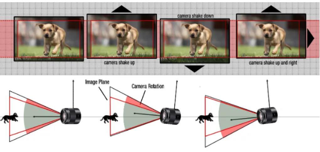
Figure 1.1 Video stabilization based on additional motion sensors. Electronic Image Stabilization (EIS) is a highly effective method of compensating for hand jitter that manifests itself in distracting video shake during playback. EIS relies on an accurate motion sensor for tracking the source of jitter,which may be hand shake or vehicle motion for example. The motion information is then integrated during the current video frame and used to compensate for it by cropping the viewable image from a stream of video frames thru the imaging pipeline. Source : TDK InvenSense solutions

for video stabilization

These instabilities can produce different types of degradation. Abrupt motion, often seen when using hand-held devices, or high-frequency tremors, such as those felt on a moving vehicle, can cause important visual discomfort [7], [8]. Lower-frequency motion, such as the up and down movements resulting from walking while filming, can distract the viewer from the focus of the video [9]. Finally, for a camera equipped with a rolling shutter sensor, fast camera movements can induce deformations in the scene [10], [11]. Digital stabilization aims at creating a new video showing the same scene but removing all these unintentional components of camera motion.

Digital video stabilization is useful in various contexts. As the production and dif-fusion of video increases, the facilitation of high-quality amateur videos becomes an important field for video-sharing platforms such as Youtube [4]. In professional contexts, law enforcement agencies have increasingly access to videos taken on the spot as evidence. Similarly, they increasingly make use of body cameras, which

(24)

1.1. Context and motivations 23

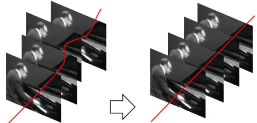
Figure 1.2 Illustration of video stabilization.Video stabilization aims at removing unintentional movements and create a smooth video.

suffer from sever shakes whenever the wearer is running [12]. Video surveillance cameras can also suffer from detrimental jitter, often due to meteorological con-ditions [13]. Stabilizing such videos can make their exploitation much easier. Other fields that can benefit from this are the medical field with camera-assisted surgery, or remote control of unmanned aerial vehicles [14]. Video stabilization also allows the separation of camera-induced motion and object-dependent mo-tion. This can serve as a pre-processing step in many video analysis processes that use object motion, such as background substraction or object tracking [13]. While digital stabilization can use additional information from gyroscopes or accelerometers [7], or different viewpoints [15] to improve or facilitate the process, most methods only rely on the video sequence taken from a single camera. Early methods used simple 2-dimensional models such as translations or similarities to represent the camera motion and remove all perceived camera motion to obtain a video corresponding to a simulated video captured by a fixed virtual camera [16]. Motion filters and path-fitting techniques have since been introduced to take intentional camera motion into account, in order to simulate professional camera movements [2]. Similarly, more complex motion models, based on structure-from-motion methods, have been proposed. These computationally demanding solutions, relying on 3-dimensional models, become now attractive and practical thanks to the current high-performance computation technologies [17]. However, computing depth from a video sequence remains a long and difficult process that fails in many situations, hence the enduring popularity of 2-dimensional models. Another type of models, that attempt to obtain visually-plausible rather than physically-accurate videos, has emerged more recently [18].

(25)

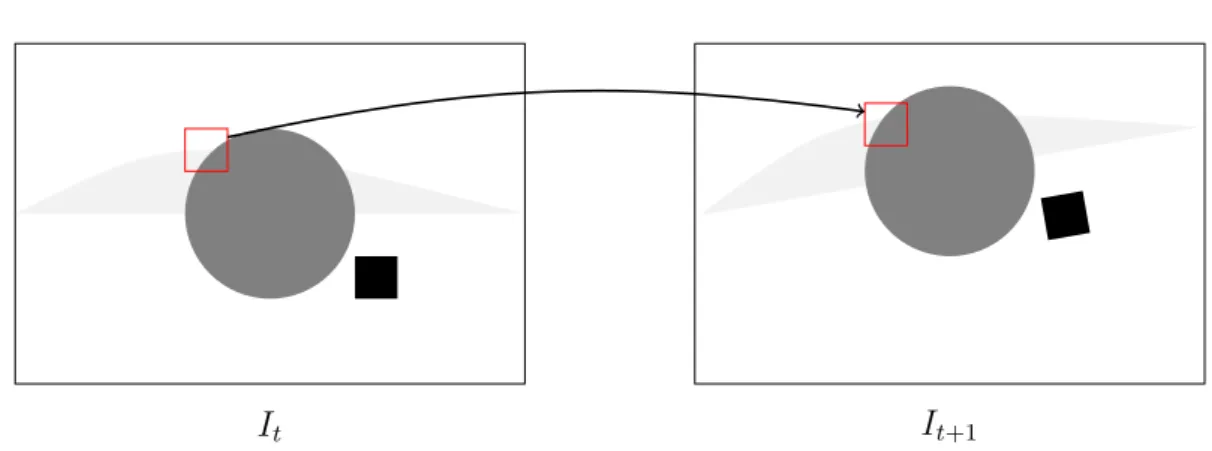
It It+1

˜ It+1

Video Stabilization

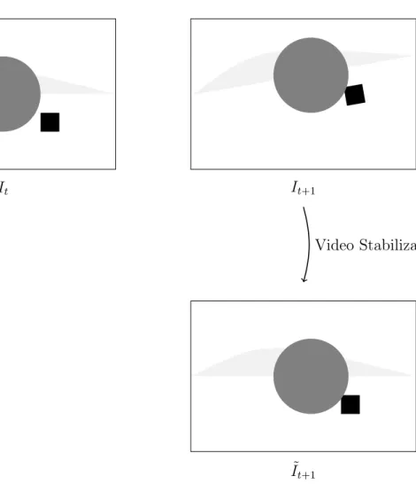
Figure 1.3 Principle of video stabilization. From frame I_t to I_t+1, the camera moves, as well as the gray circle in the foreground. Video stabilization consists in computing It+1, a new version of frame It+1 in which the static objects (here, the background)

are motionless.

1.2 Basic notions on video analysis and processing

This section describes basic notions related to video processing, that will be useful in the following manuscript.

1.2.1 Digital representations of videos

First, let us consider how videos are represented in digital format. Videos are sequences of images, called frames. Each of these frames show what the observed scene looked like at a given time t. For the sake of simplicity, we will refer from

(26)

1.2. Basic notions on video analysis and processing 25

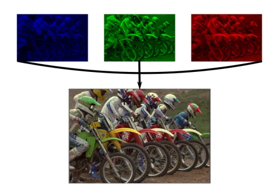
Figure 1.4 Illustration of the composition of a colour video, with the three different colour channels.

now on frame t the frame corresponding to the view of the scene at this time t. The succession of frames gives the impression of continuous movements from the series of still images. This is because the rate of succession of the frames is very rapid. This rate is noted in frame per second (fps), with most videos using 25-30 fps. In digital format, frames are represented as H × W × C matrices. H indicates the number of rows and W the number of columns in the matrix. Meanwhile, C represents the number of channels used. In the case of black and white videos, only one channel, representing the luminosity, is used. In colour videos, three channels are used to code the image in the colour-space RGB for the raw format. Figure1.4 shows the composition of an RGB image. Cases with C>3 are possible, such as videos taken with depth cameras, but are beyond the scope of this thesis. Each intersection of a row and column is called a pixel, for picture element. The dimensions H ×W of the frames composing a video is called the resolution, and indicates how precisely the scene can be rendered.

1.2.2 Pinhole camera model

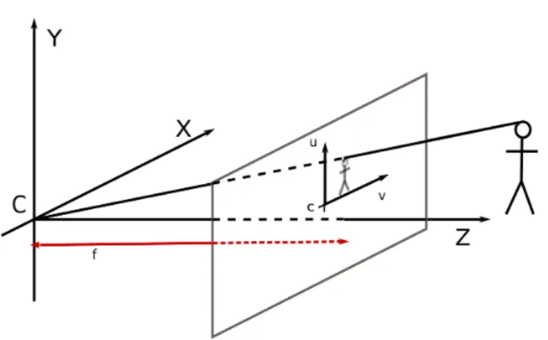
The acquisition of frames is done by projecting the 3D points of the scene onto the 2D camera plane. The link between the 3D scene coordinates (xs_{, y}s_{, z}s_{) and the}

(27)

(see Figure 1.5). If (C, X, Y, Z) is the coordinate system of the 3-dimensional space and (c, u, v) the coordinates of the camera plane onto which the image is projected, the relationship between three dimensional points and their two dimensional projection can be written as :

  U V S  = K     xs ys zs 1     (1.1)

with the relationship between the coordinates of the camera plane and the vector (U, V, S) given by:

xv = u_S

yv = V_S (1.2)

In this equation, K is a 3 × 4 matrix that describes the mathematical relationship between the coordinates of a point in three-dimensional space and its projection onto the image plane. In the simplest case, K only depends on the focal distance f , that is the distance between the image plane and the camera center C:

K =   −f 0 0 0 0 −f 0 0 0 0 1 0   (1.3)

However, this assumes that the aspect ration of the pixels is 1:1. Furthermore, it is only valid if the center of the image plane is also the origin of the coordinate system, when in practice we often use the bottom left corner of the frame as the origin. In such cases, the matrix K is described as:

K =   −f kx 0 x0 0 0 −f ky y0 0 0 0 1 0   (1.4)

In such cases, kx and ky indicate the aspect ratio of the pixels, while x0 an y0

indicate the coordinates of the new origin in the current coordinate system. The coordinates of the scene use the camera aperture as the origin, hence any motion of the camera has repercussions on the coordinates of the scene and therefore on the projected image.

1.2.3 Motion blur and rolling shutter

This acquisition is done over a slight time lapse, which can lead to sufficiently fast objects to change projection between the beginning and the end of this lapse,

(28)

1.2. Basic notions on video analysis and processing 27

Figure 1.5 Illustration of the projection onto the image plane. (C, X, Y, Z) is the 3-D coordinate system of the scene, (c, u, v) the 2-D coordinate system of the image plane

and f the focal distance.

Figure 1.6 Illustration of the rolling shutter effect. Note the tilted tower in the second frame. This is caused by fast camera movements from left to right, which causes vertical edges to be seen as diagonal as the camera changes position between

capturing successive rows.

creating what is called “motion blur". While CDD sensors capture the whole frame at the same time, CMOS sensors use instead what is called “rolling shutter": that is, frames are acquired one row at a time rather than all at once. Because of this, fast camera movements can cause deformations in vertical structures, as the camera changes position while the frame is captures. Figure 1.6 shows an exemple of rolling shutter artifact.

1.2.4 Compression and encoding

Once video frames have been captured, they are encoded in specific formats, usually with a degree of compression. The videos considered here are either in AVI or MP4 format with a variety of codec, the h264 codec being the most common. The h264 codec codes the images in the Y’CbCr color space, which uses the

(29)

luminance Y’ and the luminance with the blue and red channels subtracted (Cb and Cr respectively). However, for the treatment of video stabilization methods, frames are decompressed and converted to RGB format before being treated. The impact of compression on the stabilization results are beyond the scope of this thesis.

1.3 Contributions and publications

The contributions of this thesis are composed of three main parts :

• A didactic and structured overview of video stabilization meth-ods and current challenges. The main purpose of this contribution is to provide a fairly unifying framework to allow a better understanding of the progress of this research subject with appreciable industrial and academic benefits. This overview is focused on the main challenges, practical aspects and mathematical core concepts of the video stabilization techniques. By using a step-by-step approach, the video stabilization pipeline can be put in perspective so as to compare the main available approaches and discuss the milestones of this research area.

W. Guilluy, L. Oudre and A. Beghdadi. Video stabilization: overview, challenges and perspectives. submitted to IEEE Transactions on Circuits and Systems for Video Technology. 2018.

• A new method for outlier removal and camera motion estimation. The estimation of the 2D or 3D camera parameters from feature trajecto-ries is a tricky process since not all movements present in the video give information on the camera motion. While static objects are only affected by camera-induced movements, other objects undergo displacements that are caused by both the camera motion and the movements of the object in the scene. These moving objects need to be separated from the others and removed in order to compute the correct camera path. We propose a novel approach to assess and select the best feature trajectories to use in the cam-era motion estimation for video stabilization. Unlike standard approaches used for the selection of feature trajectories, we analyze the movement of the feature trajectories through all frames and compute a global weight by considering multiple criteria such as movement and duration.

(30)

1.4. Overview of the manuscript 29

video stabilization. In Proceedings of the European Signal Processing Con-ference (EUSIPCO). Rome, Italy. 2018.

• A new framework for the video stabilization quality assessment. To the best of our knowledge there has been very few studies dedicated to performance evaluation of video stabilization methods. The lack of such studies is mainly due to the fact that video instability, like other spatio-temporal distortions and artifacts, is very difficult to model. Indeed, the way this distortion affects the perceived quality is misunderstood and there is no way on how to quantify, in an effective way, the effect of this distor-tion on the overall quality of the video. Our contribudistor-tion in this context is twofold. First, by scrupulously reviewing all existing metrics and describing the assumptions behind them, we provide one of the first study dedicated to evaluation. Secondly, we confront existing metrics with subjective results collected on viewers so as to enlighten the existing links between objective scores and visual inspection.

W. Guilluy, A. Beghdadi and L. Oudre. A performance evaluation frame-work for video stabilization methods. In Proceedings of the European Work-shop on Visual Information Processing (EUVIP). Tampere, Finland. 2018.

1.4 Overview of the manuscript

The manuscript is organized as follows: chapter2presents an overview of previous methods of video stabilization. Chapter 3 reviews the different ways that video stabilization methods have been evaluated and presents an investigation of the performances of several video stabilization methods on a sample of those metrics, comparing them to a user study of the stabilization methods to investigate the links between the proposed metrics and the user experiences. Chapter4 present a novel selection method to identify motion caused solely by the camera motion and evaluates the impact on a standard stabilization pipeline. Finally, chapter 5

offers concluding remarks on the contributions of this work and the current state of video stabilization research.

(31)

(32)

Chapter 2 Video stabilization : challenges and

methods

(33)

(34)

33

Chapter 2

Video stabilization : challenges and

methods

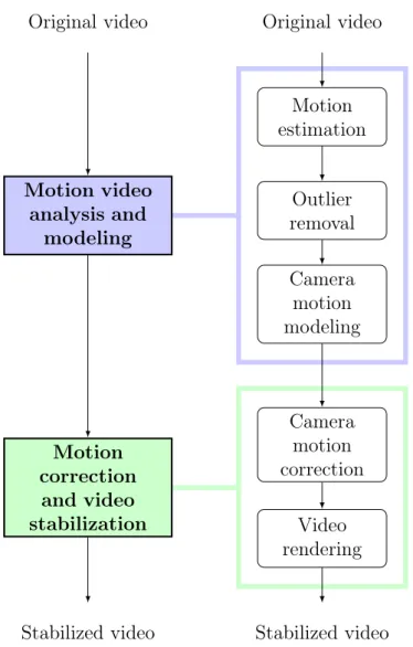
Video stabilization aims at transforming a video I corrupted by involuntary cam-era movements into a stabilized video ˜I, in which these movements are smoothed in order to produce a coherent and continuous video stream with low visual dis-comfort and better display quality. This operation is a complex process composed of many steps that could be roughly grouped into two main block as illustrated in Figure 2.1. First, the original video I is analyzed through motion estimation process. The aim of this first phase is to compute estimates of the camera move-ments from the video. In a second phase, these estimated camera movemove-ments are corrected and smoothed, as in attempt to remove their involuntary parts while preserving their voluntary parts. The video is finally processed by using the softened camera movements, so as to generate the stabilized video signal ˜I. As mentioned in Chapter1, video stabilization has been a major field of research during the last two decades due to the wide range of its potential applications. Many approaches have been introduced in the literature to solve this problem. Although based on these two general principles (analysis and correction), the methods have evolved by adding pre/post processing steps and using more pre-cise models. In particular, the level of complexity in the video analysis step has increased across the years in order to refine the estimation of the camera motion. As a result, most of current state-of-the-art methods are composed of five to ten processing blocks that are conceived to adapt to the different situations encoun-tered throughout the stabilization process and to improve the performances. In this article, we provide a structured overview of the stabilization methods pro-posed in the literature, according to the chart-flow presented on Figure 2.1. To this end, we propose to decompose each of the two main stages of video sta-bilization into a series of functional blocks, that will be studied and described individually. These functional blocks have been picked according to their popu-larity in the community and to their abilities to enlighten the different directions

(35)

34 Chapter 2. Video stabilization : challenges and methods Original video Motion estimation Outlier removal Camera motion modeling Camera motion correction Video rendering Stabilized video Motion video analysis and modeling Motion correction and video stabilization Original video Stabilized video

Figure 2.1 Main steps for video stabilization

taken in the literature. Although all these blocks are not necessary present in all published methods, they constitute a convenient way to compare the different approaches according to the same analysis grid.

The first stage of video stabilization consists in the analysis of the video. The aim is to estimate the camera motion from all the motions observed in video. In the following, we decompose this analysis stage into three main successive steps : motion estimation, outlier removal and camera motion modeling. First, the frames of the video are analyzed so as to understand all the movements in the video : this is the motion estimation step. These movements might be due to the camera or to moving objects/subjects in the scene. In order to only focus

(36)

Chapter 2. Video stabilization : challenges and methods 35

on the movements that are in fact due to the camera, the second step consists in outlier removal. Based on general assumptions on the possible impacts of camera movements on the video, this block discards all movements that are not consistent to a plausible camera displacement. Consequently, this step extracts the movements that will be useful in the stabilization process. Finally, the last block provides a camera motion modeling from the relevant movements ex-tracted from the video. As will be seen in the next section, this can be done either by assuming a geometrical model for the camera displacement (in this case the block outputs geometrical parameters for the camera), or by using an empirical model which does not take the geometrical constraints into account.

At the end of the first stage, camera motion estimates are available and can be used to process the shaky video. The second stage of video stabilization consists in the processing of the video. More specifically, the camera motion models output by the first stage go through a correction process so as to reconstruct a more pleasing video. In the following, we decompose this processing stage into two main successive steps : camera motion correction and video rendering. The first block performs a camera motion correction by smoothing and filtering the camera movements. Whether geometrical parameters of the camera are available or not, the correction step aims at suppressing the involuntary camera movements and to compute a new plausible camera motion. In this step, the strength of the stabilization can also be adjusted so as to provide pleasing results for the viewer. Finally, the new camera movements are applied back to the original disturbed video, within the video rendering step. This final step reconstructs a new video with smoothed camera movements.

In the following, for the sake of completeness and clarity, the video stabilization process is presented as a set of interdependent steps described in the order they appear in the whole VS pipeline. First, the video analysis step consists of esti-mating motions present in the video (Section2.1), then identifying those resulting from the motion of the camera (Section2.2) to be used to model the original path of the camera (Section 2.3). The video is then stabilized by correcting the path of the camera (Section 2.4) and rendering a video (Section 2.5), simulating the scene as captured by a virtual stabilized camera following the corrected path.

Notations

The aim of this whole process is to transform a video sequence I containing unintentional camera movements into a stabilized sequence ˜I. In the following, let zt, [xt, yt, 1] be a pixel belonging to frame t and It(zt) the luminance channel

(37)

36 Chapter 2. Video stabilization : challenges and methods Motion estimation Pixel-based Block-matching Feature-based KLT SIFT SURF Others

Figure 2.2 Main approaches for motion estimation

2.1 Motion estimation

The first step of any video stabilizer is to acquire knowledge of the camera move-ments. However, in the context of digital stabilization, no direct information about the camera is known, since only the video sequence is available. Motion estimation aims to recover movements present in the video sequence, which will be used to determine the motion of the camera. These movements are estimated by searching for correspondences between consecutive frames. Pixels (or blocks of pixels) from the first frame are matched with the pixels (or blocks of pixels) in the following frame if they are assumed to correspond to the same element within the captured scene. Several approaches have been introduced to solve this problem: some try to find a match for every pixel in the frame (Section 2.1.1), others use blocks of pixels (Section 2.1.2) and finally, points of interest can be used to estimate the movements (Section 2.1.3).

2.1.1 Pixel-based matching

Pixel-matching methods seek to determine the motion of pixels between two frames [19]. As illustrated in Figure 2.3, each pixel of the first frame corre-sponds to the projection of a 3D point in the observed scene onto the camera plane, and is matched by the pixel of the following frame corresponding to the projection of the same 3D point onto the new camera plane [20]. To determine this point-to-point correspondence, the luminance of any given object is assumed to be constant throughout a video sequence. Therefore, such methods attempt to match pixels with the same intensity. However, many pixels in a given pair of frames may have similar intensity; therefore additional constraints are needed to obtain a unique solution [21], [22]. Early methods suppose that the movements

(38)

2.1. Motion estimation 37

It It+1

Optical flow

Figure 2.3 Principles of optical flow. Optical flow aims at computing the displacement of each pixel between frame It and It+1. It is often displayed as a vector field.

are predominantly caused by the motion of the camera, which is modeled by a 2D transformation. Such methods, instead of computing the displacement for ev-ery pixel, search for the transformation parameters that best explain the overall displacement of the frame. Those parameters are easily estimated by minimiz-ing the luminance difference between the two adjacent frames [23].If Ht denotes

the transformation matrix between the frames t and t + 1, the best parameters minimize the differences ||It(Htzt) − It+1(zt+1)||2 for all pixels. Robust functions

have also been used to make this approach more robust to outliers [24]. This ap-proach solves simultaneously the different steps of the camera motion modeling. This saves times, but needs a pre-determined motion model. Since only adjacent frames can be compared, there is not enough information to solve a 3D motion model, constraining the results to 2D models. In addition, this cannot be used with an outlier removal scheme. It is also sensitive to changes in illumination. A recent method [25] uses a similar approach to identify the correction directly, using the pixel matches as one component of an energy function using neural networks.

(39)

38 Chapter 2. Video stabilization : challenges and methods

It It+1

Figure 2.4 Principles of block matching. Block matching aims at computing the displacement of blocks of pixels between frame Itand It+1.

Another approach is to determine the optical flow between adjacent frames. Op-tical flow consists in finding the displacement field (ut, vt) of each pixel ztbetween

two consecutive frames It and It+1. These displacements are estimated thanks to

several assumptions, such as that neighbouring pixels have similar movements [26] or that the flow is smooth or piece-while smooth [27]. The flow is often computed iteratively using the spatial and temporal gradients[28]. The main advantage of using optical flow is that it recovers a dense flow field, which is necessary for some stabilization methods [29] or for enhancements such as in-painting [30]. Another advantage is that neighbourhood relations are easy to determine between motion vectors, which can be exploited in later steps [31]. However, computing dense optical flow may require heavy computations. This can be partially alleviated by using other faster matching methods to compute an initial flow before running the iterative algorithm [32]. Another option, which has been used in real-time applications [3], is to use sparse optical flow, which do not solve for motion in low-gradient areas. The main drawback of optical flow is the running time: this is often the longest operation in a video stabilization process that uses it, as the movements from easily matched features must be propagated to flat spaces. Liu et al. [29] report 1.1 seconds per frame to compute the optical flow out of 1.5 sec-onds per frame for the whole stabilization algorithm. In addition, times is spent calculating the optical flow on features that have their own movement in addition to the camera’s, and therefore are hard to use to evaluate the camera’s move-ments. Finally, because motion vectors are determined for pixel coordinates and not for specific features, trajectories of objects or features cannot be determined.

(40)

2.1. Motion estimation 39

2.1.2 Block-matching

Instead of finding correspondences between pixels, block-matching methods use blocks of pixels of size (2n+1)×(2n+1) and estimate their displacements between adjacent frames, as illustrated on Figure2.4. The use of blocks allows to remove some ambiguities that appear when matching individual pixels, by decreasing the chance of several matches being detected. Furthermore, by assuming that motion between two frames is limited, it is possible to only consider blocks of pixels within a certain search radius of the block to be matched, further restricting the possibilities for matches. The best displacement (ux, uy, 1) for a given pixel (zt =

(xt, yt, 1)) is the one minimizing the energy E , with the considered displacements

(ux, uy, 1) smaller than the given search radius.

E(xt, yt, ux, uy) = n X k=−n n X l=−n ||It(xt+ k, yt+ l, 1) − It+1(xt+ ux+ k, yt+ uy+ l, 1)||2 (2.1) To that end, block-matching approaches are based on search windows that con-strain the possible motions. This is computationally very efficient, but two main problems emerge. First, the aperture problem caused by the search windows: smaller windows run the risk of being too small to contain the true motion, while larger windows are prone to containing several possible matches. Secondly, ho-mogeneous surfaces have little to promote one match over another. These regions are therefore often dropped from computing the displacement, and are consid-ered ambiguous. The result is a motion field presenting similar advantages to the optical flow fields, with easy neighbourhood relations but no object trajectories. The main disadvantages is that untextured areas are not filled in.

2.1.3 Feature-matching

Feature matching seeks to identify points in the scene that are easily recognizable. In this case, only the displacements of these points of interest are computed, as illustrated on Figure 2.5. By processing the entire video frame after frame, the positions of these points can be tracked using the properties of the given features, forming trajectories. One of the advantages of using this approach is that the same point can be tracked and recognized across many frames, from the frame it is originally identified to the frame where it is no longer present. In particular, the study of the trajectories can give a better insight on the movements present in the scene.

A commonly used [10], [11], [13], [14], [17], [18], [33], [34] tracking algorithm is the KLT tracker [35]. A feature detection algorithm is used to initialize the position

(41)

It It+1

Figure 2.5 Principles of feature point matching. Feature point matching aims at computing the displacement of only a subset of relevant pixels between frame It and

It+1.

of tracked points, which are then tracked using optical flow. A confirmation check verifies that the feature has been tracked correctly, otherwise the feature trajectory is ended. New feature points can be detected in later frames if too many feature points have been lost.

SIFT points are also widely used [2], [36]–[39]. These features use descriptors based on the image gradient to obtain very specific descriptors that make matches very reliable. The descriptors contain the orientation of the feature in order to be rotation-invariant, and detection is used at several image scales that help avoid problems caused by zooming, although it is slower than most alternatives. SURF points were designed on similar principles [40], but optimized for speed, making them a good alternative [41]–[43]. SIFT features have also been used in conjunc-tion with line detecconjunc-tion methods [44], as deformations caused by stabilization are particularly visible on lines.

Other features used include Maximally Stable Extremal regions (MSER) [45] or FAST corners using BRIEF descriptors [12], [46]. MSER detect contiguous re-gions whose borders are darker/brighter than any pixel in the region. An ellipse is then fitted over the region, using the covariance matrix to identify the ellipse axis in order to make it rotation-invariant. FAST corners are detected when a contigu-ous number of pixels are darker or lighter by a tolerance threshold compared to the central pixel, and descriptors are based on binary comparisons between the cen-tral pixel and the rest of the patch. FREAK descriptors [47] have also been used in

some recent works Zhao2019TrajDerivatives. These binary descriptors use overlapping samples similar to the distribution of retinal cells in the human eye., [48], [49]

Feature-matching provides accurate and fast results, and the obtained trajecto-ries allow for additional temporal analysis in the remaining steps of the process,

(42)

2.2. Outlier removal 41

Outlier removal

Frame-to-frame analysis

Video stream analysis

Figure 2.6 Main steps for outlier removal

although scenes with large uniform regions can sometimes yield few features per frame. However, because features are spread unevenly across the video frames. This can lead to some areas being over-represented in the motion analysis. Fur-thermore, neighbourhood relations are harder to establish.

2.2 Outlier removal

While all movements observed in the video sequence are affected by the motion of the camera, not all observed movements are suitable to determine the camera motion. The presence of moving objects in the filmed scene can be a source of errors, as the movements of the objects could be mistaken for those caused by the camera motion. Errors can also occur while determining the movements in the video sequence. Finally, some movements may be too complex for a given motion model. Detecting and removing such movements is important to ensure accu-rate camera motion analysis. Therefore, several methods use a post-processing step after the movement estimation [50], that are designed to remove these out-liers. Two main approaches can be used, that are either based on frame-to-frame analysis (Section 2.2.1) or on the whole video stream (Section 2.2.2).

2.2.1 Frame-to-frame analysis

Most outlier detectors consider two adjacent frames and label as outliers all the displacements that do not fit the general observed movement. This can be done by computing the fitting error between the estimated camera model and the individual movements in the video. If the majority of movements are caused solely by the camera motion, they are assumed to fit the camera motion model, and those deviating from the model are considered unreliable.

The most commonly used method is the RANSAC algorithm [51]. Using a given motion model, RANSAC randomly selects data to determine the model parame-ters and measures the distance between the expected positions and the observed

(43)

positions, with a threshold determining whether a given point is considered inlier or outlier. The parameters resulting in the fewest outliers are selected. Different variants on RANSAC have been used. For instance, umLESAC uses preliminary tests before measuring the fitting error to discard bad data samples quickly and adapts the number of iterations to the dataset [52]. Another variant, ORSA, uses an a contrario approach to avoid a hard threshold on the fitting error [53]. This approach has the advantage of solving for camera motion and detecting outliers at the same time. But it can led astray if the majority assumption is false for a single frame.

Assumptions on camera motion can also be used to determine outliers. One hypothesis is that objects in the scene move faster than the camera. Outliers are detected simply by thresholding the velocity of the observed movements [45]. Another hypothesis, in the case of dense optical flow, is to consider the smoothness of the flow field. Thresholding the spatial gradient of the vertical and horizontal flow fields detects the edges of moving objects, and by successive iteration can remove all flow vectors corresponding to moving objects [29]. Median filters can also be applied, on both fine scale to remove tracking errors and small moving object, then on a larger scale to remove larger outliers [54]. Finally the spatial distribution can be taken into account. For instance, a RANSAC variant applies a grid over the reference frame and limits the number of movements selected from one quad for any iteration of RANSAC [34], which avoids over-fitting the model to a specific area of the frame. Using a similar grid, RANSAC can be applied separately to each quad, resulting in local outlier detection [4]. Because only adjacent frames are used, this approach can be applied in real-time without requiring a buffer. It can also be used with any type of motion detection methods.

2.2.2 Video stream analysis

Outlier detection can also take into account motion over more than two frames. This allows the consideration of the evolution of motion vectors over time, how-ever it requires tracking points over show-everal frames. Trajectories recovered using feature point tracking is often used in this regard. One criteria that can be ex-ploited is the difference between expected and observed motion. In particular, the motion induced by the camera has been modeled as a projection into a low rank subspace. Trajectories whose projections differ strongly from the original motion at any given time are considered faulty and discarded [18]. similarly, if the RANSAC algorithm has been used to determine an initial transformation, then the differences between the known positions of features and the expected positions can be computed [48]. These differences, called projection errors, can be used to refine the outlier rejection. Trajectories that repeatedly cause large

(44)

2.3. Camera motion modeling 43 Camera motion modeling 2D models 3D models Perceptual Affine Homography Others

Figure 2.7 Main approaches for camera motion modeling

projection errors can then be reclassified as outliers. In addition, trajectories that have been often classified as outliers can be excluded from the initial RANSAC execution and reclassified as inliers only if they have small projection errors. Ob-serving trajectories over a given temporal window can also give insight on which trajectories are the most reliable. Firstly, some approaches require trajectories of a minimum length, such as models using epipolar geometry [55], which require temporally distant frames to work. Trajectories that do not span the required frames are therefore considered outliers. Methods that work directly on trajec-tories may require a minimum length for a trajectory to be usable, and need to augment some trajectories that are too short, in which case it is logical to pri-oritize the trajectories requiring the least degree of interpolation [11]. Finally, moving objects often leave the frame quickly as they pass through the scene, so longer trajectories are prioritized as more likely to belong to the static back-ground of the scene [18]. The spatial distribution can also be exploited over a period of time. Bi-layer clustering is a method used to detect large moving ob-jects in the foreground of videos. It uses motion and colour to segment feature trajectories into two clusters, and chooses to remove the cluster with the greater compacity, as the background of a scene is far less compact than moving objects [11]. These methods are only applicable if feature trajectories have been obtained using feature-matching while detecting motion in the video.

2.3 Camera motion modeling

Once outliers have been removed, the remaining movements are the result of the camera motion. They can therefore be used to model or approximate the camera motion. To that end, two strategies can be used. In most works, the modeling of the camera motion is based on geometrical models that describe the physical process of capturing a scene with a pinhole camera. Early works have proposed to use 2D models that approximate the effects of camera motion on

(45)

the movements of pixels in the video (Section 2.3.1). By recovering the depth information and using 3D models, it is also possible to seek for the original 3D displacements of the camera (Section 2.3.2). Alternatively, another approach is to avoid geometrical models to obtain perceptually plausible models, in order to obtain visually acceptable corrections rather than physically accurate ones (Section 2.3.3).

2.3.1 2D models

As such, the physical movement of the camera lies in a 3D space. However, the influence of the camera movements is only accessible through the frames of the video, i.e a 2D space. This is why 2D models approaches do not attempt to recover the original 3D path of the camera but model its influence between two frames as a 2D transformation. More specifically, considering two successive frames Itand It+1, and a pixel zt , [xt, yt, 1] belonging to frame t, its coordinates

zt+1 in frame t + 1 are given by

zt+1= Htzt (2.2)

where Ht is a 2D-transformation matrix describing the motion between frames t

and t + 1. The general form of matrix Ht,

Ht=   h11 h12 h13 h21 h22 h23 h31 h32 1  , (2.3)

allows to consider several types of 2D transformations such as pure translation, pure rotation, similarity, affinity or homography. 2D approaches have been really popular for their simplicity of use and low computational cost [16]. They do not require the challenging task of depth estimation, and provide, in case of low parallax or small relative depth variations, a fast and robust way of determining camera movements [24], [56]. Moreover, the 2D assumption is often valid on a local temporal scale when the movements of the camera are not to large. They can also be computed from frame-to-frame correspondences, and can thus be used in conjunction with any type of motion detection. Finally, the parameters of the transformation and the pixel position are enough to determine the expected location of the pixels after applying camera motion. This means that the motion caused by the camera is known for every pixel and the corrections required can likewise be known exhaustively.

(46)

2.3. Camera motion modeling 45

The simplest parametric planar transforms to be considered are the similarities (also referred to as simplified affine models) [16]. They are able to handle trans-lations, scaling and rotation along the camera axis and are based on only four parameters a, b, tx, ty such that

Ht=   a −b tx b a ty 0 0 1  . (2.4)

Parameters a and b handle the scaling the rotation along the roll-axis, while tx

and ty respectively model the horizontal and vertical translations. By setting

a = λ cos(θ) and b = λ sin θ, the scaling/rotation effects can be specified with λ the scaling parameter and θ the rotation parameter [57]. The estimation of the four parameters can be solved by linear Least Squares Method on a set of redun-dant equations [36], [58], [59], possibly combined with filtering/outlier removal [32], [42]. Histogram approaches have also proven to be effective in this context [60], [61]. Empirical studies have shown that, in videos acquired with hand-held cameras, most of the involuntary movements such as vibrations are considered significant in the place perpendicular to the z-axis [56]. These results allow to think that by only considering scale, z-axis rotation, and translations, it is possi-ble to obtain an acceptapossi-ble approximation [6], since the impact of pitch and yaw rotations on the final image warping are often minimal for this kind of videos. Furthermore, due to its low number of parameters to be estimated, the similarity model constitutes a relevant solution for real-time applications [3]. The similarity model also presents the advantage of introducing very little deformations, which makes it robust to outliers and noise [62]. However, it cannot account for strong rotations outside of the camera axis , which may limit its performances in strongly degraded videos.

Slightly more complex with six parameters, the affinity (or generalized affine model) is the most commonly used 2D model. By replacing parameters a and b by four parameters a11, a12, a21, a22 the matrix transformation writes

Ht=   a11 a12 tx a21 a22 ty 0 0 1  . (2.5)

The affinity model encompasses most of the qualities of the similarity model, but additionally allows the possibility of shear [9], [37], [44], [46]. The parameters can be estimated with standard differential motion techniques [23], with more complex cost functions [24] or through multi-scale [63] or hierarchical analysis [30], [64]. The major advantage of using an affinity model lies in the fact that it naturally handle global motions, for which the affinity parameters at every

(47)

location should be the same [65]. The model can deal with scenes containing small relative depth variations and zooming effects [38] and provides an acceptable compromise between accuracy and computational cost[45]. However, being a 2D planar transform, it cannot model non-linear inter-frame motion [4].

Finally, the most exhaustive 2D is the homography, which uses 8 parameters. The matrix transform becomes

Ht =   a11 a12 tx a21 a22 ty a31 a32 1  . (2.6)

While the interpretation of the coefficients is not as straightforward as for simi-larity or affinity [2], they control rotations, translations, zooming and sheering in the x- and y- axis [66]. Homographies have been popular for image registration [53], and most authors use techniques developed in this context for the estimation of the eight parameters [13], [14], [44]. Nevertheless, the homography model has the potential to cause severe deformations, particularly in the presence of outliers [12].

Other 2D models include simpler models with 3 [62], [67], [68] or 4 parameters (2 rotations and 2 translations) [69]. So-called 2.5D models propose to compromise between 2D and 3D models, by considering cases where 3D displacements can be simplified to avoid the need for depth (translations 1 axis (x, y or z)) [70].

2.3.2 3D models

Contrary to 2D models, 3D models aim at recovering the actual original 3D displacement of the camera, which is represented by a single point, according to the standard pinhole camera assumption. Instead of only considering the influence of the camera motion in the 2D plane, the 3D models are able to provide physically realistic displacements in all the directions. Their ability to compute a precise estimation of the movement is dependant on the depth recovery step, i.e the estimation of the distance to the camera of each 3D point seen in the frames [55], [71]. Recovering depth consists in analyzing the original video (where the available information lies in 2D planes), in order to retrieve the original 3D content of the scene. This task, referred to as structure-from-motion [17], often uses groups of 3 key-frames and estimates the parametric 3D transformation that best fit the observed movement. In practice, the computation of the model may be subject to numerical instabilities, especially if the movement is not strong enough. To that end, it is common to use distant key frames, that insure that sufficient motion is present. This is only possible using feature trajectories, as it is the only

(48)

2.3. Camera motion modeling 47

motion estimation method that can match points across distant frames. Even so, if the motion contains no depth differences and/or no translations, numerical instabilities are inevitable. To handle this issue, some recent works propose to add geometrical constraints in the model (existence of planes [72], manifold constraints [73]) that help to provide accurate computation. The computation cost, which is often high, can be be kept under control by only focusing on particular regions of interest [74], [75]. Because of this, the depth is usually only recovered for certain pixels, which leads to incomplete motion fields and corrections.

The main drawbacks of 3D models can also be taken into account by building hybrid models that combine 2D models (which are efficient, easy to compute but imprecise) and 3D models (which are physically accurate but tricky to compute). To that end, some methods propose to only consider certain displacements in the 3D space. For instance, by considering only rotations, it is possible to drop the depth recovery task and only focus on the estimation of the calibration ma-trix and the rotation mama-trix [7], [10]. This assumption appears to be valid for hand-held shakes but is violated in more complex conditions such as walking or driving. In the context of moving vehicles, plausible movements are limited to rotations and translation in the direction of the car displacement. By using these constraints, it is possible to simplify the general 3D model and provide ad hoc for-mulation that are lighter than structure-from-motion [8]. Finally, some authors propose to introduce the notion of 2.5D models, and to define ad hoc models that correspond to classical situations (dolly, vertical or horizontal tracking...). The specification of the movements helps to compute the depth estimation and can therefore provide accurate results.

2.3.3 Perceptual models

As seen in the previous subsections, there are many different motion models to choose from. The choice of the appropriate model can be tricky when no extra information is available on the camera movement, which unfortunately is often the case. Moreover, models perform very differently depending on the scene and the camera motion, and choosing an inappropriate model can have severe repercussions on the stabilization results [18]. Several approaches have been proposed to try to combine the robustness and computational efficiency of 2D models with the accuracy of 3D models. Such approaches have in common an important principle : the main objective of video stabilization is to improve visual comfort. As a result, these methods prefer to avoid geometrical models and instead use models that provide visually plausible videos rather than physically accurate ones. Such models are referred to as perceptual models. While their

Video stabilization : A synopsis of current challenges, methods and performance evaluation

HAL Id: tel-03006243

https://tel.archives-ouvertes.fr/tel-03006243

Video stabilization : A synopsis of current challenges,

methods and performance evaluation

Wilko Guilluy

To cite this version:

Université Paris 13

Doctoral Thesis

Video stabilization : A synopsis of

current challenges, methods and

performance evaluation

Author:

Wilko Guilluy

Abstract

Résumé en français

Remerciements

Contents

List of Figures

List of Tables

Chapter 1

Introduction

Chapter 1

Introduction

1.1

Context and motivations

1.2

Basic notions on video analysis and processing

1.2.1

Digital representations of videos

1.2.2

Pinhole camera model

1.2.3

Motion blur and rolling shutter

1.2.4

Compression and encoding

1.3

Contributions and publications

1.4

Overview of the manuscript

Chapter 2

Video stabilization : challenges and

methods

Chapter 2

Video stabilization : challenges and

methods

Notations

2.1

Motion estimation

2.1.1

Pixel-based matching

2.1.2

Block-matching

2.1.3

Feature-matching

2.2

Outlier removal

2.2.1

Frame-to-frame analysis

2.2.2

Video stream analysis

2.3

Camera motion modeling

2.3.1

2D models

2.3.2

3D models

2.3.3

Perceptual models