Investigation of Ethernet switches behavior in presence of contending flows at very high-speed

(1)

a p p o r t

d e r e c h e r c h e

IS S N 0 2 4 9 -6 3 9 9 IS R N IN R IA /R R --L IP 2 0 0 6 -3 8 --F R + E N G Thème NUM

Investigation of Ethernet switches behavior in

presence of contending flows at very high-speed

Sebastien Soudan — Romaric Guillier — Ludovic Hablot — Yuetsu Kodama — Tomohiro Kudoh — Fumihiro Okazaki — Pascale Primet — Ryousei Takano

N° 6031

(2)

(3)

Unité de recherche INRIA Rhône-Alpes

655, avenue de l’Europe, 38334 Montbonnot Saint Ismier (France)

Téléphone : +33 4 76 61 52 00 — Télécopie +33 4 76 61 52 52

Sebastien Soudan∗_{, Romaric Guillier}∗_{, Ludovic Hablot}∗_{, Yuetsu Kodama}†_{, Tomohiro}

Kudoh†_{, Fumihiro Okazaki}†_{, Pascale Primet}∗_{, Ryousei Takano}†

Thème NUM — Systèmes numériques Projet RESO

Rapport de recherche n° 6031 — November 2006 — 23 pages

Abstract: This paper examines the interactions between layer 2 (Ethernet) switches and TCP in high bandwidth delay product networks. First, the behavior of a range of Ethernet switches when two long lived connections compete for the same output port is investigated. Then, the report explores the impact of these behaviors on TCP protocol in long and fast networks (LFNs). Several conditions in which scheduling mechanisms introduce heavy unfair bandwidth sharing and loss burst which impact TCP performance are shown.

Key-words: ethernet switches, queue management, transport protocol, cross-layering.

This text is also available as a research report of the Laboratoire de l’Informatique du Parallélisme

http://www.ens-lyon.fr/LIP.

∗

LIP, UMR INRIA-CNRS-ENS Lyon-UCB Lyon 5668 †

(4)

haut débit

Résumé : Ce rapport présente les interactions entre les switchs de couche 2 (Ethernet) et TCP dans

les réseaux à haut produit débit-délai. Tout d’abord, nous investiguons le comportement de plusieurs switches Ethernet lorsque deux connexions se partagent un même port de sortie. Nous explorons en-suite l’influence de ces comportements sur le protocole TCP. Enfin nous exhibons plusieurs situations dans lesquelles le mécanisme d’ordonnancement introduit un partage inéquitable de la bande passante et des pertes en rafales pénalisant les performances de TCP.

(5)

1 Introduction

Most transport protocol designers addressing wired networks do not take link layer behaviors into account. They assume a complete transparency and determinist behavior (i.e. fairness) of this layer. However, Ethernet switches are store-and-forward equipments, which have limited buffering capaci-ties to absorb congestions that can brutally occur, due to bursty nature of TCP sources [JD05]. Thus many Ethernet switches use contention algorithms to resolve access to a shared transmission chan-nel [FKM04, AOST93, McK99]. These scheduling algorithms aim at limiting the amount of data that a subnet node may transmit per contention cycle. This helps in avoiding starvation for other nodes. The designers of these algorithms have to find a tradeoff between performance and fairness in a range of traffic conditions [MA98]. Considering the case of grid environment where many huge data transfers may occur simultaneously, we explore the interactions between this L2 congestion control mechanisms and TCP and try to understand how they interfere. The goal of this study is to investigate the way packets are managed in high speed L2 equipments (switches) and the implication on transport protocols under different congestion conditions. The question is to understand how the bandwidth and losses are distributed among flows when traffic profiles correspond to huge data transfers.

After a brief introduction on switching algorithms, the second section of this paper details the experimental protocol adopted and the observed parameters. In the third part, we present the steady-state behaviors of CBR (Constant Bit Rate) flows’ packet scheduling and the switch’s characteristic. In the fourth section, this report study the impact on this kind of flows and on TCP. The report ends by a discussion on the problems of switching algorithms in grid context.

2 Switching algorithms

Switching algorithms are designed to solve contentions that may occur on output ports of a switch when several inputs ports intend to send packets on the same port. In input-queued switches, this problem is known as head of line blocking problem. There are mainly two types of such algo-rithms. Some use a random approach by choosing randomly packets among contending input ports as PIM [AOST93] does whereas others (as iSLIP [McK99]) use round-robin. From a global point of view, both can achieve fairness among input port but from a local point of view results can be quite different [Var05, chapter 13].

A user doesn’t know a priori which algorithms are used in its switches nor if they are of one of these two types.

3 Experiment description

In order to observe the bandwidth sharing and loss patterns on a congested output port of a switch, a specific testbed and a restricted parametric space were used to explore 1 Gbps Ethernet port behavior.

3.1 Objectives and Test plan

In order to characterize the switches and the impact of switches on TCP, several experiments have been performed.

The first set of experiments consists of running two contending flows at different constant rates. These two flows permit to observe different behaviors of the switch under different congestion level, to highlights the difference of behaviors of different switches using mean and variance of per-flow

(6)

output bandwidth. Fine-grained observation can also be made using sequence numbers to observe per-packet switching behaviors in presence of two flows.

Then as TCP tends to send packets per bursts, experiments with one CBR flow and one burst are run. The number of packets of the burst is observed as a function of burst’s length.

And lastly two different variants of TCP (BIC and Reno) are evaluated on two different switches. Performance are measured under different situations: with and without SACK as it is designed to improve TCP performance under specific loss pattern and with a 0 ms and 50 ms RTT GigE link as TCP’s performance are impacted by losses and high latencies.

These experiments are run the testbed describe in the next section.

3.2 Testbed

The topology of the experimental testbed is described on figure 1. One GtrcNET-11 [KKT+

03] is used to both generate traffic and monitor the output flows. GtrcNET-1 is an equipment made at the AIST which allows latency emulation, bandwidth limitation, and precise per-stream bandwidth mea-surements in GigE networks at wire speed. GtrcNET-1 has 4 GigE interfaces (channels). Tests were performed with several switches but most of the results presented here are based on a Foundry Fast-Iron Edge X424 and a D-Link DGS1216-T. Firmware version of the Foundry switch is 02.0.00aTe1. “Flow control” is disabled on all used ports and priority level is set to 0. According to manufacturer’s

documentation, D-Link has 512 KB and according to command line interfaceshow memcommand,

Foundry switch has 128 MB of RAM but for both the way memory is shared among ports is not known. GtrcNET−1 Switch ch1 GtrcNET−1 ch3 ch2 flow 1 flow 2 GtrcNET−1 ch0

Figure 1: Experimental testbed

3.3 Parametric space

We assume L2 equipments do not differentiate UDP and TCP packets. Tests that have been made corroborate this fact. Experiments were conducted with UDP flows as they can be generated easily by GtrcNET-1 and as they can be sent at a constant rate.

(7)

The following parameters were explored: flows’ rate, packet length and measure interval length. Different levels of congestion using different flow’s rates were used : 800, 900, 950 and 1000 Mbps. These rates are transmission capacity (TC) used to generate UDP packets. Transmission capacity specify the bitrate (including Inter Frame Gaps and preamble) of an emulated Ethernet link. Experi-ments were strictly included in the period of packet generation. IP packet length are set to 1500 bytes as high-speed connections use full size packets. In order to observe output flow bandwidths, packets

were counted on intervals of 400 and 1000µs (around 33 and 83 packets at 1 Gbps).

3.4 Test calibration

We first compare the flows generated by GtrcNET-1 with and without switch to be sure switches do

not introduce too much noise. Here, the observation interval is 400µs.

With 1000 Mbps (wire speed) as transmission capacity, due to preamble and IFG, transmission

bandwidth will be of 1000 ∗ (64 + 18)/(64 + 18 + 20) = 803 Mbps with 64 bytes packets and

1000 ∗ (1500 + 18)/(1500 + 18 + 20) = 986 Mbps with 1500 bytes packets. Table 1 summarizes

these values.

GtrcNET-1’s is able to generate packets at the specified rates. When GtrcNET-1’s channel 3 (ch3) is directly connected to ch0 and ch3 generates UDP packets, monitored bandwidth on ch0 is constant. Then, the measurements with one flow transiting through the Foundry Fast IronEdge X424 switch was done. Figures 3 represent the output bandwidths observed on ch0 when the flow goes through the switch. In these figures, measured bandwidths are not as stable as the ones obtained without switches (figure 2) but the obtained rates are nearly the same.

Transmission capacity (Mbps) UDP bandwidth (Mbps) 64 B packets 1500 B packets

900 724 888

950 764 937

1000 803 986

Table 1: UDP flows bandwidth with respect to transmission capacity used

0 200 400 600 800 1000 0 0.1 0.2 0.3 0.4 0.5 0.6 0.7 0.8 0.9 bandwidth (Mbps) time (s) flow

(a) IP length = 64 bytes

0 200 400 600 800 1000 0 0.1 0.2 0.3 0.4 0.5 0.6 0.7 0.8 0.9 bandwidth (Mbps) time (s) flow (b) IP length = 1500 bytes

Figure 2: Without switch, TC = 1000

(8)

0 200 400 600 800 1000 0 0.1 0.2 0.3 0.4 0.5 0.6 0.7 0.8 0.9 bandwidth (Mbps) time (s) flow

(a) IP length = 64 bytes

0 200 400 600 800 1000 0 0.1 0.2 0.3 0.4 0.5 0.6 0.7 0.8 0.9 bandwidth (Mbps) time (s) flow (b) IP length = 1500 bytes Figure 3: Switch, TC = 1000

4 Steady-state behaviors of CBR flows’ packets scheduling

This section presents some of the bandwidth patterns observed on the output port of the Foundry Fast IronEdge X424 switch when two CBR (Constant Bit Rate) flows are sent through this output port. We only concentrate on 1500 bytes packets as high throughput flows use such packets size (or over with jumbo frames). Each figure of this section represents the output rate of the two flows (subfigures (a) and (b)). Sums of output bandwidths are always constant at 986 Mbps. Measures presented in this section are made using 1 ms intervals.

4.1 Two CBR flows with same rates

Figures presented in this section use the same input rate for the two flows.

In figure 4, only one flow is forwarded at a time. There are many transitions between the two flows but it seems to be completely random. It can be noticed that the aggregated bandwidth is nearly constant and that one flow can starve for more than 100 ms (for example: flow 1 between 1.6 s and 1.7 s). 0 200 400 600 800 1000 0 0.5 1 1.5 2 2.5 bandwidth (Mbps) time (s) flow 1

(a) Output bandwidth of flow 1

0 200 400 600 800 1000 0 0.5 1 1.5 2 2.5 bandwidth (Mbps) time (s) flow 2

(b) Output bandwidth of flow 2

(9)

In figure 5, flows do not starve but a real unfair sharing is observed for more than 300 ms. From time 1.45 s to 1.75 s, one is running at more than 900 Mbps and the other at less than 50 Mbps.

Figure 5: 900 Mbps + 900 Mbps (1500 bytes)

As seen in all the figures shown in this section, sharing among input ports can be really unfair on “short” time scale, which can have a dramatic impact as 100 ms may be a very long interval within TCP’s dynamic specifically at these rates. Around 8300 1500-bytes packets should have been forwarded at 1 Gbps within 100 ms.

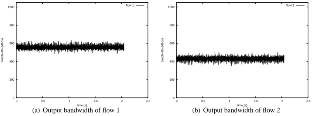
4.2 Two CBR flows with different rates

In figure 6, it can be observed that when the two flows are sending at different rates (with one at wire speed), instant flow rate on the output port varies among a set of values. And finally, when none of the flows is at 1 Gbps and they have not the same rate, as in figure 7, the sharing of the bandwidth is closer to what we would expect to obtain as with 1 ms interval observation the throughput is nearly constant. 0 200 400 600 800 1000 0 0.5 1 1.5 2 2.5 bandwidth (Mbps) time (s) flow 1

As a conclusion of this section, when the two CBR flows have the same rate or one of the flow is at the maximum rate, the behavior of this switch is unfair on “short” time scale (100 ms) but is not

(10)

when none of the two rates is at wire rate. The following sections present some quantitative measures on these situations for several switches.

4.3 Sequence number analysis

In this section, instead of monitoring the output bandwidth, the sequence numbers of forwarded pack-ets are monitored. Figure 8 shows the situation with two 1000 Mbps flows and figure 9 with two 400 Mbps flows on Foundry switch. In these figures is the sequence number of a packet at the date it was observed on the output port represented by an impulse. It can be noticed that on the first figure (figure 8), only one flow is forwarded at a time most of the time just like observed in figure 4, whereas on the second ones (figure 9) output packets are picked alternatively from the two flows (figure 9 (c) is a zoom-in of a short interval).

0 10000 20000 30000 40000 50000 60000 70000 80000 90000 0 0.1 0.2 0.3 0.4 0.5 0.6 0.7 0.8 0.9 1 Sequence number time (s)

(a) Sequence number of flow 1

0 10000 20000 30000 40000 50000 60000 70000 80000 90000 0 0.1 0.2 0.3 0.4 0.5 0.6 0.7 0.8 0.9 1 Sequence number time (s)

(b) Sequence number of flow 2

Figure 8: Evolution of sequence number of packets on the output port (1000 Mbps + 1000 Mbps (1500 bytes) on Foundry switch)

On D-Link switch, even when the two input rates are 1000 Mbps (figure 10), packets on output port come alternatively from the two port but packets are alternatively dropped too. Sequence numbers of forwarded packets are growing by from 1 to 3 (figure 10 (c)) as there is only 1000 Mbps of bandwidth on output port and some of the input’s packets have to be dropped. This is different from the Foundry switches where packets are dropped by burst. The case with 400 Mbps flows and D-link is similar to Foundry one. This likely means the two tested switches have different queue management strategies.

(11)

0 5000 10000 15000 20000 25000 30000 35000 0 0.2 0.4 0.6 0.8 1 1.2 Sequence number time (s)

0 5000 10000 15000 20000 25000 30000 35000 0 0.2 0.4 0.6 0.8 1 1.2 Sequence number time (s) 0 5000 10000 15000 20000 25000 30000 35000 0 0.2 0.4 0.6 0.8 1 1.2 Sequence number time (s) 0 5000 10000 15000 20000 25000 30000 35000 0 0.2 0.4 0.6 0.8 1 1.2 Sequence number time (s)

90 100 110 120 130 140 150 160 170 180 0.005 0.00505 0.0051 0.00515 0.0052 0.00525 0.0053 0.00535 0.0054 Sequence number time (s) flow 1 flow 2

(c) Zoom with both flows

Figure 9: Evolution of sequence number of packets on the output port (400 Mbps + 400 Mbps (1500 bytes) on Foundry switch)

0 10000 20000 30000 40000 50000 60000 70000 80000 90000 0 0.2 0.4 0.6 0.8 1 1.2 Sequence number time (s)

410 400 390 380 370 360 350 340 330 320 310 300 290 280 270 260 250 240 230 0.005 0.00505 0.0051 0.00515 0.0052 0.00525 0.0053 0.00535 0.0054 Sequence number time (s) flow 1 flow 2

(c) Zoom with both flows

Figure 10: Evolution of sequence number of packets on the output port (1000 Mbps + 1000 Mbps (1500 bytes) on D-Link switch)

4.4 Quantitative measures for CBR flows

Following tables summarize statistical metrics for the two flows on different switches with different input rates. The first two columns indicate the input rates in Mbps for flow 1 and flow 2, the next four columns show average, maximum and minimum throughput (Mbps) and its variance (square Mbps) for flow 1. The next four do the same for flow 2 and finally the last column indicates the interval used for throughtput measurements.

It can be observed that tables 2, 3 and 4 show a very high variance and minimum throughput of 0 Mbps when the input rates are equal to 1000 Mbps whereas table 5, 6 and 7 don’t. The three first switches are tend to make one of the flows starve for periods of time longer than 100 ms when the congestion is severe. These three switches also perform unfair sharing under high congestion whereas the three last always split the available bandwith around 494 Mbps when the input rates are equals. In the case of D-Link switch, it occurs even when the input rates are different and the output port is congested.

To conclude this section, it seems switches divide in two different classes. In the first one star-vation can occur and high variance under severe congestion can be experienced. In the second one low variance and no starvation occurs. As TCP connections have no knowledge of which switches the network is made of, it can be guessed that the behavior and performances of the connections can be highly and differently impacted as it will be shown in section 5.

(12)

Input rate ch0(flow 1) ch0(flow 2)

Interval

CH2 CH3 ave max min var ave max min var

1000 1000 800 988 666 19K 188 323 0 19K 100 ms

800 800 197 197 197 0 792 791 792 0 100 ms

References

[AOST93] Thomas E. Anderson, Susan S. Owicki, James B. Saxe, and Charles P. Thacker. High-speed switch scheduling for local-area networks. ACM Trans. Comput. Syst., 11(4):319– 352, 1993.
[FKM04] Morteza Fayyazi, David Kaeli, and Waleed Meleis. Parallel maximum weight bipartite
matching algorithms for scheduling in input-queued switches. IPDPS, 01:4b, 2004.
[JD05] Hao Jiang and Constantinos Dovrolis. The origin of TCP traffic burstiness in short time
scales. In IEEE INFOCOM, 2005.
[KKT+
03] Y. Kodama, T. Kudoh, T. Takano, H. Sato, O. Tatebe, and S. Sekiguchi. GNET-1: Gigabit ethernet network testbed. In Proceedings of the IEEE International Conference Cluster
2004, San Diego, California, USA, September 20-23 2003.
[KT05] Anshul Kantawala and Jonathan Turner. Link buffer sizing: A new look at the old
prob-lem. In ISCC ’05: Proceedings of the 10th IEEE Symposium on Computers and
Com-munications (ISCC’05), pages 507–514, Washington, DC, USA, 2005. IEEE Computer
Society.
[MA98] Nick McKeown and Thomas E. Anderson. A quantitative comparison of iterative
schedul-ing algorithms for input-queued switches. Computer Networks and ISDN Systems,
30(24):2309–2326, December 1998.
[McK99] Nick McKeown. The iSLIP scheduling algorithm for input-queued switches. IEEE/ACM
Trans. Netw., 7(2):188–201, 1999.
[MHR03] Matt Mathis, John Heffner, and Raghu Reddy. Web100: extended TCP instrumentation
for research, education and diagnosis. SIGCOMM Comput. Commun. Rev., 33(3):69–79, 2003.
[TKK+
05] R. Takano, T. Kudoh, Y. Kodama, M. Matsuda, H. Tezuka, and Y. Ishikawa. Design and evaluation of precise software pacing mechanisms for fast long-distance networks. In
In Proceedings of the International workshop on Protocols for Long Distance Networks (PFLDNET), Lyon, France, 2005.
[Var05] George Varghese. Network Algorithmics: an interdisciplinary approach to designing fast
networked devices. Elsevier, 2005.
[XHR04] Lisong Xu, Khaled Harfoush, and Injong Rhee. Binary increase congestion control for
fast long-distance networks. In IEEE INFOCOM, 2004.
Unité de recherche INRIA Futurs : Parc Club Orsay Université - ZAC des Vignes 4, rue Jacques Monod - 91893 ORSAY Cedex (France)
Unité de recherche INRIA Lorraine : LORIA, Technopôle de Nancy-Brabois - Campus scientifique 615, rue du Jardin Botanique - BP 101 - 54602 Villers-lès-Nancy Cedex (France)
Unité de recherche INRIA Rennes : IRISA, Campus universitaire de Beaulieu - 35042 Rennes Cedex (France) Unité de recherche INRIA Rocquencourt : Domaine de Voluceau - Rocquencourt - BP 105 - 78153 Le Chesnay Cedex (France)
Unité de recherche INRIA Sophia Antipolis : 2004, route des Lucioles - BP 93 - 06902 Sophia Antipolis Cedex (France)
Éditeur
INRIA - Domaine de Voluceau - Rocquencourt, BP 105 - 78153 Le Chesnay Cedex (France)
http://www.inria.fr