Zigzag instability of a chi disclination line in a cholesteric liquid crystal

HAL Id: ensl-00182727

https://hal-ens-lyon.archives-ouvertes.fr/ensl-00182727

Submitted on 26 Oct 2007

HAL is a multi-disciplinary open access

archive for the deposit and dissemination of

sci-entific research documents, whether they are

pub-lished or not. The documents may come from

teaching and research institutions in France or

abroad, or from public or private research centers.

L’archive ouverte pluridisciplinaire HAL, est

destinée au dépôt et à la diffusion de documents

scientifiques de niveau recherche, publiés ou non,

émanant des établissements d’enseignement et de

recherche français ou étrangers, des laboratoires

publics ou privés.

cholesteric liquid crystal

Alain Dequidt, Patrick Oswald

To cite this version:

Alain Dequidt, Patrick Oswald. Zigzag instability of a chi disclination line in a cholesteric liquid

crystal. European Physical Journal E: Soft matter and biological physics, EDP Sciences: EPJ, 2006,

19 (4), pp.489-500. �ensl-00182727�

Zigzag instability of a χ disclination line in a cholesteric liquid

crystal

A. Dequidta

and P. Oswaldb

Laboratoire de Physique de l’Ecole Normale Sup´erieure de Lyon, 46 All´ee d’Italie, 69364 Lyon Cedex 07, France Received 16 January 2006 /

Published online: 13 April 2006 – c° EDP Sciences / Societ`a Italiana di Fisica / Springer-Verlag 2006 Abstract. We studied the formation of χ disclination lines in planar cholesteric samples placed in a tem-perature gradient near the cholesteric to smectic A phase transition. We observed that the first simple line which forms close to the smectic-cholesteric front zigzags when it is perpendicular to the direction of planar anchoring and is straight for other orientations. This instability is similar to Herring instability for crystalline surfaces. We show numerically that it originates from a strong increase of the elastic anisotropy close to the transition. In addition, we propose a new method to measure the pitch divergence at the smectic to cholesteric phase transition.

PACS. 61.30.Jf Defects in liquid crystals – 64.70.Md Transitions in liquid crystals

1 Introduction

It was known for a long time that the surface energy γ of a crystal depends on its orientation with respect to the underlying lattice. For this reason, the equilibrium shape of a monocrystal is not spherical but anisotropic with flat facets and rounded parts (respectively “smooth” and “rough” at the atomic scale). It may also happen that certain faces are missing in the equilibrium shape, which leads to angular edges (or points). Smectic B plastic crys-tals are of this type as faces perpendicular to the smectic layers (or close to these orientations) are missing [1]. From a thermodynamical point of view, these orientations cor-respond to metastable or unstable states. In the unstable case, the surface stiffness, given by eγ = γ+d2

γ/dθ2

(where θ is an angle defining the crystallographic orientation of the face) is negative (for a demonstration, see Ref. [2]). What happens, now, if one forces such an orientation to appear? The answer was given in 1951 by Herring [3], who showed that the surface must destabilize and recon-struct into a hill-and-valley recon-structure. This phenomenon is variously referred to as “thermal faceting,”“Herring re-construction,” or“hill-and-valley reconstruction” by met-allurgists [4]. In solids, this instability has been observed on high-index surfaces of certain metals and semiconduc-tors at high temperatures [5, 6]. Unfortunately, this pro-cess is very slow because it requires material transport by diffusion over large distances [7]. For this reason, only the first stages of the reconstruction have been observed.

Her-a

e-mail: [email protected]

b

e-mail: [email protected]

ring instability was also studied at the smectic B-smectic A interface [8, 9] in a temperature gradient G. In these con-ditions, a hill-and-valley structure (very close to a zigzag) forms, with a wavelength proportional to G−1/3 _in

agree-ment with theory.

It turns out that dislocations in solids can also zigzag due to an instability similar to Herring instability. In-deed, let us consider a dislocation pinned at its ends A and B. In very anisotropic crystals such as semiconduc-tors, it frequently happens that the dislocation line ten-sion along direction AB (a quantity strictly equivalent to the surface stiffness of a crystalline surface) is negative. In this case, the line is unstable and takes, at equilib-rium, a“polygonal” shape, the more marked, the higher the anisotropy [10].

Analogous instability has been observed in nematic and cholesteric liquid crystals either. In these materials, the first observation is certainly due to the Orsay Liquid Crystal Group who observed in 1969 that double χ discli-nation lines of cholesteric phases form a zigzag when they are submitted to a strong enough magnetic field [11, 12]. The same year, Kl´eman and Friedel [13] proposed that this instability was originating in the special pair structure of these lines and was due to a change of sign of their line tension under magnetic field. Another, more recent, exam-ple concerns disclination lines of strenght 1/2 which form in flat capillary tubes treated for homeotropic anchoring. In that case, the line zigzags because of a “partial escape” of the director parallel to its axis [14]. Zigzagging disclina-tion lines were also observed in biaxial lyotropic nematic

Fig. 1. χ disclination line in a cholesteric liquid crystal (from Ref. [17]).

liquid crystals [15]. Finally, zigzag instability of a“splay-bend” Ising wall was reported very recently [16].

A common point to several of these experiments (and that we shall discuss later in this article) is the key role played by the elastic anisotropy in the appearance of the instability.

In the present article, we return to simple χ disclina-tion lines in a cholesteric liquid crystal and show that they can spontaneously destabilize in the vicinity of a smectic A phase. Such a line forms at the frontier between two domains containing different numbers of half-pitches. We recall that a cholesteric liquid crystal is a chiral nematic twisted in a single direction, while the smectic A phase has a lamellar structure [17]. A cholesteric is character-ized by its pitch p which is the distance over which the director rotates by 2π. Because ~n ⇔ −~n (~n is the di-rector), the true periodicity is the half-pitch. In practice, χ disclination lines are observed in a “Grandjean-Cano wedge” (for a review, see Ref. [17]). In this geometry, the cholesteric is sandwiched between two glass plates mak-ing a small angle and treated for planar anchormak-ing in the same direction. Due to this angle, the number of half-pitches within the sample thickness is not constant and increases from one side of the sample to the other. Let us denote by h(x) the sample thickness (with the x axis perpendicular to the wedge). It can be shown that, at equilibrium, simple χ disclination lines (Fig. 1) form at thicknesses h(xm) = (2m − 1)(p/4) with m = 1, 2, · · · .

An alternative way to observe the lines is to place a sam-ple of constant thickness in a temperature gradient. If the pitch changes sufficiently with temperature, lines form in the sample perpendicularly to the temperature gradient. This systematically happens close to a smectic-cholesteric phase transition because the pitch strongly increases [18– 20]. In practice, both methods can be mixed, which we did indeed experimentally. Surprisingly, we observed that the first line which develops close to the smectic A-cholesteric front can destabilize for some orientations with respect to the planar anchoring by forming a zigzag reminiscent of Herring instability.

The plan of the article is as follows. In Section 2, we de-scribe the experiment and the main observations. In Sec-tion 3, we show how to measure by extrapolaSec-tion the pitch as a function of temperature very close to the transition toward the smectic phase. In Section 4, we describe in more detail the instability of the first simple line (m = 1). In Section 5, we calculate numerically its line tension as a function of the angle θ that the line makes with the an-choring direction of the molecules on the glass plates. We show that the instability develops when θ approaches π/2, in agreement with experiments, and is due to the diver-gence of the bend elastic constant close to the transition. Concluding remarks are drawn in Section 6.

2 Experimental setup and preliminary

observations

The liquid crystals chosen are two mixtures of 8CB (4-octyl-40_{-cyanobiphenyl) with the chiral molecule ZLI 811}

from Merck (0.45 wt% and 0.15 wt%, respectively). At these concentrations the pitch is inversely proportional to the concentration. These two mixtures have a cholesteric-smectic A phase transition at about T ≈ 33.2◦_{C. The}

samples are sandwiched between two rectangular glass plates of size 2 × 3 cm and of thickness 1 mm. Both plates are treated for strong planar anchoring. The anchoring is achieved by depositing a layer of PVA (polyvinyl al-cohol) by spin-coating on the glass plates. Each layer is dried and polymerized during 40 minutes at 125◦C and, then, rubbed in a single direction (parallel to one edge of the plates) with a nylon fiber cloth placed on a rotating cylinder. Two nickel wires parallel to the short edge of the plates are used to fix the sample thickness. In general, their diameters are different which leads to a wedge geom-etry. The thickness h(x) along the x axis perpendicular to the wedge is measured by imaging with a high-resolution camera the fringes of equal thickness which form in the re-flecting microscope under normal illumination. The sam-ple is placed into a cell consisting of two ovens maintained at different temperatures. It can be moved inside the cell owing to a step-by-step motor acting on a micrometric screw via a speed reducer, and its position is measured with a linear position sensor within ± 5µm. The ovens im-pose to the sample a temperature gradient ~G which has been previously calibrated with a dummy sample con-taining a thermocouple. Finally, the sample can rotate inside the cell which allows us to fix the angle between the temperature gradient ~G and the thickness gradient ~g = (dh/dx)~x. A schematic representation of the exper-imental configuration is shown in Figure 2 (for a more detailed description of the cell, see Ref. [21]).

In practice, the temperatures of the two ovens are cho-sen in such a way that the smectic-cholesteric front and the χ lines that form in its vicinity sit in the gap between the two ovens to be observable under the microscope. A photograph is shown in Figure 3. In this case, ~g k ~G, with the temperature and the thickness decreasing from left to right, and θ = 0 (planar anchoring direction parallel to the

Fig. 2. Schematic representation of the experiment. When ~

G k ~g, the χ lines are parallel to the smectic front. In most of our experiments, the planar anchoring direction is either parallel or perpendicular to ~G.

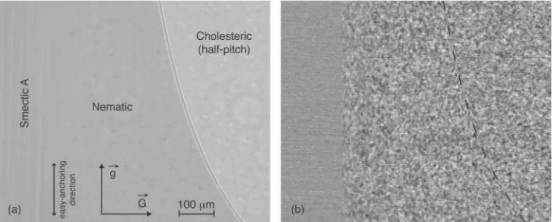
Fig. 3. χ disclination lines observed near the smectic-cholesteric front when the planar anchoring direction is per-pendicular to ~G (θ = 0). All the lines are stable. The dashed line marks the position of the smectic front: at this place, the sample thickness is 18 µm (natural light, 0.45 wt%, g = 13.3 µm/cm, G = 5◦_C/cm).

lines). For this orientation, all the lines are stable. In addi-tion, it can be checked experimentally that the cholesteric is completely unwound and forms a planar nematic phase between the smectic front and the first line (line 1). On the other hand, the director rotates by π within the sample thickness between lines 1 and 2, and again by π between lines 2 and 3, etc.

The situation changes completely when θ approaches π/2. In this case, the first line develops a zigzag instability as shown in Figure 4, whereas other lines remain perfectly straight. This instability of line 1 will be described in more detail in Sections 4 and 5.

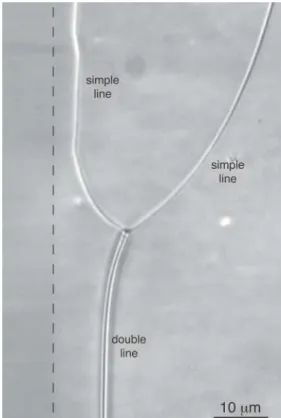
We also observed once a transient configuration in which the first two lines had merged to form a double line (Fig. 5). This configuration was unstable, as the double line tends to shorten, becoming progressively replaced by the two usual lines. In addition, we see in this photograph

Fig. 4. First χ line forming a zigzag when the planar anchor-ing direction is parallel to ~G (θ = π/2 in average). Note the difference of grey levels between the smectic A and the ne-matic phases. At the position of the line, the sample thickness is equal to 10 µm (polarizer and analyzer uncrossed, 0.45 wt%, g = 4.6 µm/cm, G = 2◦_C/cm).

Fig. 5.Unique example of two simple lines merging into a dou-ble line. This configuration is transient, with the doudou-ble line tending to shorten to be slowly replaced by the two simple lines. The dashed line marks the position of the smectic to nematic front. The thickness is approximately equal to 35 µm (un-crossed polarizers, 0.45 wt%, g = 20 µm/cm, G = 50◦_C/cm).

Note that all the experimental conditions were met to favor the nucleation of double lines (in particular, a large thickness gradient was used).

that the usual line close to the smectic front was unstable, whereas the other two (and, in particular, the double one) were stable. This observation is important as it shows that in our experiments, we had to deal with simple lines.

In the following section, we show how to measure the pitch as a function of temperature close to the smectic phase. The non-trivial role of the temperature gradient is emphasized and a new method of measurement is pro-posed.

Fig. 6.a) Wedge sample in a temperature gradient perpendicular to the thickness gradient. In this configuration, the line bends and shifts from the smectic front. The thinner the sample, the larger the effect. In this photograph, the line is clearly visible but the smectic front is almost invisible; b) To see the smectic front, we subtracted two images taken at 0.1 s interval. This technique allows us to visualize both the front and the line. For more clarity, we superimposed a dashed line to the line on the picture (0.15 wt%, G = 12.5◦_{C/cm, g = 12 µm/cm, and h = 12 µm in the middle of the photo).}

3 Pitch measurement

In the classical Grandjean-Cano method, the pitch is mea-sured by placing a wedge sample in an oven maintained at a constant temperature T and by measuring the sam-ple thickness h(xm) at the place xm of the m-th line.

Indeed, it can be shown that, at constant temperature, h(xm) = (2m − 1)(p/4), where p is the cholesteric pitch

at temperature T (for a demonstration, see, for instance, Ref. [17]). This method allows a direct determination of p(T ) and has been widely used in the past.

The determination of p(T ) is a bit subtler when the sample is placed in a temperature gradient. Indeed, let us consider the first line and let us suppose it is stable (no zigzag). The problem which now arises is to determine its position x1 with respect to the smectic front assumed to

be located at x = 0. At vanishingly small temperature gra-dient (G → 0), we already know that p(T ) = h(x1)/4 with

x1= (T − T_{N A})/G. In practice, x1, h(x1) and G are

mea-sured, which allows, in principle, a precise determination of p(T ). The problem is that the relation p(T ) = h(x1)/4

fails when G 6= 0 because the line energy depends on the temperature via the Frank elastic constants. To show this, let us denote by E1(T ) the line energy and by h = h(x1)

the local sample thickness, supposed to be constant (this is true within an excellent approximation because x1 varies

very little in comparison to the sample length when G is changed). In order to calculate the line position x1 with

respect to the smectic front, let us calculate the total en-ergy of the cholesteric phase. It reads:

Etot(x1) = h Z x1 0 1 2K2(x)q(x) 2 dx +h Z L x1 1 2K2(x) µ q(x) − π_h ¶2 dx + E1(x1) (1)

with L the size of the sample, q(x) = 2π/p(x) the equilib-rium twist of the cholesteric phase, and K2(x) the twist

constant (with the two latter quantities being taken at

temperature T corresponding to position x). Note that in this equation, the first two terms represent, respectively, the twist energy of the cholesteric phase supposed to be unwound on the left of the defect (x < x1) and to be

wound with a constant twist π/h on the right (x > x1);

as for E1(x1) it represents the line energy, which includes

the core energy and the excess of elastic energy due to the twist, bend and splay deformations induced by the defect. In the following, we shall assume that the line energy only depends on the temperature at position x1 and is thus

independent of the temperature gradient. This assump-tion is correct in our experiments as the elastic constants change very little over the typical width of the defect (of the order of p/4 as can be seen from the numerically cal-culated director fields shown in Fig. 17).

Minimization of Etot(x1) with respect to x1 gives

π q(x1) K2(x1) − 1 2K2(x1) π2 h + dE1 dx (x1) = 0. (2) In principle, this equation allows us to calculate the posi-tion (or, equivalently, the temperature) of the line in the temperature gradient G.

Experimentally, x1 can be measured under the

micro-scope, which gives the line temperature T1 for a given

temperature gradient. The temperature T1is a solution of

the following equation, equivalent to equation (2): p(T1) − 2hp(T1) π2_K 2(T1) dE1 dT (T1) G = 4h, (3)

where p(T1) is the pitch at temperature T1. So, plotting

T1 as a function of the temperature gradient G, and then

extrapolating this curve to G = 0, give the pitch at the extrapolated temperature T10= T1(G → 0):

p(T10) = 4h. (4)

To test this method and explore a large range of thick-nesses with the same wedge sample, we oriented the latter

Fig. 7. Line temperature as a function of the temperature gradient for four different thicknesses (0.15 wt%).

in the cell so that ~g⊥ ~G. In addition, we chose the pla-nar anchoring direction parallel to ~g in order to avoid the zigzag instability. In this orientation, the first line bends in the temperature gradient as shown in Figure 6. In the left photograph taken in polarized light, the line is well visible and can be easily detected. On the other hand, the smec-tic front is very difficult to localize. In order to improve its detection, we took two images of the same zone at 0.1 s interval and subtracted them. The result is shown beside the photograph: the smectic front is now clearly visible as it marks the limit between a “granular” zone (due to the nematic fluctuations) and another much smoother (corre-sponding to the smectic phase). Because the disclination line is also visible in this picture (this is due to the fact that the camera saturates on the line, which eliminates the noise), the latter can be used to measure simultaneously the front and the line positions and, consequently, the line temperature as a function of the sample thickness (for a given temperature gradient). By performing the experi-ment at different temperature gradients, we can plot, for each thickness h, the line temperature T1 as a function of

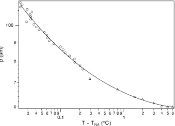
G and, then, extrapolate each curve to G = 0. Such curves are shown in Figure 7. Each extrapolated temperature gives the pitch (equal to 4h according to Eq. (4)) at this temperature. The curve p(T ) obtained in this way is shown in Figure 8 (circles). This method is particularly efficient to measure the pitch in the close vicinity of the transition temperature. To obtain points at higher temperature, far from TN A, we used the classical method consisting of

mea-suring the position of the line (and so the local thickness) in wedge samples maintained at a constant temperature (G = 0). These points are also reported in Figure 8 (tri-angles). This curve shows that the pitch tends to diverge close to TN A. As in references [18–20], we plotted our data

to a law of type p(T ) = a + bT + c(T /TN A− 1)−ν. The

solid line in Figure 8 is the best fit to this law. It gives the critical exponent ν = 0.41 ± 0.05. This value is signifi-cantly smaller than all the values given earlier for esters of cholesteryl and their mixtures (0.65 < ν < 1.2, [18–20]). Nevertheless, we emphasize that our measurements are consistent with the fact that the pitch diverges as K2 as

Fig. 8.Pitch as a function of temperature. Circles have been obtained by the extrapolation method in a temperature gradi-ent, whereas triangles have been measured in samples at con-stant temperature. The solid line is the best fit to a law of type p(T ) = a + bT + c(T /TN A− 1)−ν (0.15 wt%).

proposed by Alben on the basis of a molecular model [22]. To prove this point, let us recall that K2 diverges in the

nematic phase as ξ2

⊥/ξk [23], where ξ⊥ and ξk are the

smectic correlation lengths perpendicular and parallel to the director. As these two lengths diverge close to TN A

as (T /TN A− 1)ν⊥ and (T /TN A− 1)νk, respectively, we

must have ν = 2ν⊥ − νk. It turns out that X-ray [24]

and calorimetric measurements [25] in 8CB have given νk = 0.67 ± 0.03 and ν⊥ = 0.51 ± 0.03. From these

val-ues we calculate ν = 0.35 ± 0.09, in agreement, within experimental errors, with our findings, ν = 0.41 ± 0.05. Note that, in spite of the fact that νkand ν⊥are certainly

not universal exponents, our value of ν is close to the av-erage value of 2ν⊥− νk measured in 26 other materials:

2ν⊥− νk= 0.44 ± 0.12 [26].

In the following section, we return to zigzag instability.

4 Zigzag instability

4.1 Experimental observations

When θ = π/2 in average, the first line forms a sym-metric zigzag as already shown in Figure 4. Experiments indicate that the zigzag stabilizes after half a day, typi-cally. After equilibration, we observed that the angle θ0

between a “zig” (or a “zag”) and the planar anchoring direction (see Fig. 9a) slowly increases when the ature gradient increases (i.e., when the average temper-ature of the line T1 increases), whereas the wavelength

λ decreases in the same conditions. Temperature T1,

an-gle θ0, and wavelength λ are plotted in Figures 10, 11,

and 12, respectively. These graphs show that, for a given thickness, δT = T1− TN Avaries linearly with G, whereas

θ0 and λ may be reasonably fitted to power laws. In

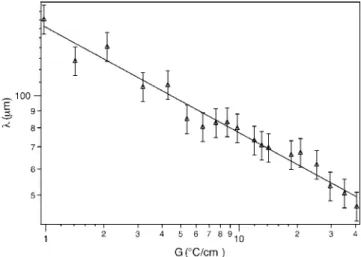
par-ticular, Figure 12 (plotted in logarithmic scale) shows that λ ∝ Gn _{with n ≈ 0.32 ± 0.02, which is very close to 1/3.}

Fig. 9.a) Symmetric zigzag when the planar anchoring direc-tion is parallel to ~G (θ = 90◦_{in average). On this photograph,}

θ0 ≈ 80◦; b) Asymmetric zigzag observed in the same

sam-ple rotated by about 5◦ _{in the temperature gradient (i.e., for}

θ ≈ 85◦ _{in average). In that case, we still measure θ} 0 ≈ 80◦

(natural light, 0.45 wt%, G = 2.1◦_{C/cm, g = 21 µm/cm,}

h = 20 µm).

Fig. 10. Average line temperature as a function of the tem-perature gradient. The line is the best fit of experimental data to a linear law (0.45 wt%, g = 21 µm/cm, h = 20 µm).

Fig. 11. Angle θ0 as a function of the temperature gradient.

The line is the best fit of experimental data to a power law (0.45 wt%, g = 21 µm/cm, h = 20 µm).

Fig. 12. Zigzag wavelength as a function of the temperature gradient. The line is the best fit of experimental data to a power law (0.45 wt%, g = 21 µm/cm, h = 20 µm).

In addition, we observed that the zigzag becomes asymmetric when the sample is slightly rotated in the temperature gradient, on condition that θ be (in average) larger than θ0. This is shown in Figure 9b. In this case,

each segment of the line (“zig” or “zag”) still makes the same angle θ0 with respect to the anchoring direction as

in the symmetric case.

Finally, the zigzag disappears when θ is smaller than θ0. In the following, we shall only consider the symmetric

case for which systematic measurements were done. 4.2 Zigzag angle calculation

In the introduction, we have recalled that a line is ab-solutely unstable when its line tension, given by τ (θ) = E1(θ) + d

2

E1/dθ 2

, is negative. Indeed, let us suppose that the line (perpendicular to the x axis) undulates according to equation x = ² sin(ky), with ² → 0. A calculation of the total energy of the undulating line per unit length along the y axis, of definition:

Etot= 1 λ Z λ 0 s 1 + µ dx dy ¶2 E µ θ + dx dy ¶ dy (5)

gives after expanding E1(θ + dx/dy) to second order in ²:

Etot= E1(θ)+ k2 ²2 4 (E1(θ)+d 2 E1/dθ 2 ) = E1(θ)+ k2 ²2 4 τ (θ). (6) As a consequence, the energy decreases when the line ten-sion is negative, which defines a criterion of absolute in-stability for the line.

Let us now return to our experiment. When ~g k ~G, the line is straight in average, but develops a zigzag when θ = π/2, which means that its line tension is negative for this orientation: τ (π/2) < 0. In addition, experiments show that each line segment (of type “zig” or “zag”) makes an angle θ0which increases and tends to 90◦ when the

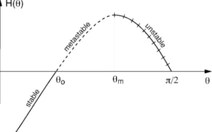
Fig. 13. Schematic representation of the function H(θ) when the line develops a Herring instability. The cross-hatched part of the curve corresponds to unstable orientations; the part in dashed line corresponds to metastable orientations; the rest of the curve in solid line corresponds to stable orientations.

express that the zigzag energy per unit length along y, of expression E1(θ)/ sin θ, is minimal for θ = θ0. That gives

d dθ µ_E 1(θ) sin θ ¶ (θ = θ0) = E0 1(θ0) sin θ0 − E1(θ0) cos θ0 sin2θ0 = 0 (7) or, equivalently, H(θ0) = E10(θ0) sin θ0− E1(θ0) cos θ0= 0. (8)

This equation yields angle θ0provided that the line energy

E1(θ) is known at the line temperature T1. This function

and angle θ0 will be calculated numerically in Section 5.

To conclude this subsection, let us analyze the func-tion H(θ). Because E0

1(π/2) = 0 by symmetry, we have

necessarily H(π/2) = 0. By contrast, H(0) < 0 because E1(0) > 0. Finally, H0(θ) = τ (θ) sin θ, which shows that

H0_{(π/2) < 0 since the line is unstable along this direction}

(τ (π/2) < 0). These considerations allowed us to plot H(θ) in a schematic way in Figure 13. This graph shows the existence of two particular angles: the zigzag angle θ0, for which H(θ) vanishes, and a larger angle, θm, for

which H(θ) passes through a maximum while the line tension changes sign.

In conclusion, this analysis shows that the zigzag angle θ0 is smaller than the smallest angle θ_m above which the

line is completely unstable. In our experiment, θ0 and θm

are very close, which explains why the shape is very close to a zigzag. In the next subsection, we calculate the zigzag wavelength.

4.3 Wavelength calculation

Before calculating the wavelength, let us generalize equa-tion (2) which gives the average posiequa-tion x1of the zigzag

in the temperature gradient (Fig. 14). Let E0be the line

energy for orientation θ0. To simplify, we assume that θ0

is constant along the zigzag, which is well verified exper-imentally. One thus obtains the line position by simply

Fig. 14. Schematic representation of the zigzag. The dashed line marks the average position of the zigzag in the tempera-ture gradient. Zones in light grey are not twisted enough. By contrast, dark-grey zones are too much twisted.

replacing E1(x1) by E0(x1)/ sin θ0 in equation (1).

Mini-mization with respect to x1then gives

π q(x1) K2(x1) − 1 2K2(x1) π2 h + 1 sin θ0 dE0 dx (x1) = 0 (9) or, equivalently, π q(T1) K2(T1) − 1 2K2(T1) π2 h + G 1 sin θ0 dE0 dT (T1) = 0 (10) These two equations generalize equations (2) and (3) to a symmetric zigzag. In the following, we choose the origin of the x axis in order that x1= 0.

We can now calculate the zigzag wavelength. To do this, we must balance three terms:

1. The twist energy lost in the regions that lie between the line and its average position at x = 0 (grey regions in Fig. 14).

2. The variation of line energy due to the temperature gradient.

3. The energy of the point defects which form between “zigs” and “zags.”

The first term reads per unit length along the y axis: h∆f1i = 4 λ Z λ 4 tan θ0 0 ∆f (x) µ_λ 4 − x tan θ0 ¶ dx (11) with ∆f = ·₁ 2K2(x)q 2 (x) − 1 2K2(x) µ_π h− q(x) ¶2¸ h = πK2(x) 2 · 2q(x) −π_h ¸ . (12)

Note we did the integration over a quarter of a wavelength (between the two vertical bars in Fig. 14), which is allowed by symmetry and providing that we can linearize the dif-ferent quantities around x = 0 (see later).

The second term writes in the form h∆f2i = 4 λ Z λ 4 tan θ0 0 E0(x) − E0(0) cos θ0 dx. (13)

The third one is simply given by h∆f3i =

2E∗

where E∗ _{is the point defect energy between a “zig” and}

a “zag.”

To calculate explicitly these three terms, we now lin-earize ∆f (x) and E0(x) around x = 0. That gives

∆f (x) = ∆f (0) + Gax, (15)

where a is a constant, measurable experimentally (see later), of expression a = d dT · πK2(T ) 2 µ 2q(T ) −π_h ¶¸ T =T1 . (16)

Because K2q is independent of temperature (see Sect. 3),

this formula simplifies and becomes a ≈ − ·_π2 2h dK2(T ) dT ¸ T =T1 . (17)

As for the line energy, it can be expressed in the form E0(x) = E0(0) +

dE0

dx x. (18)

From the latter equation together with equations (9) and (12), we calculate:

E0(x) − E0(0) = −x sin θ0∆f (0). (19)

The total energy per unit length along the y axis is obtained by replacing ∆f (x) and E0(x) − E0(0) by their

expressions (15) and (19) in equations (11) and (13), and then by summing h∆f1i, h∆f2i, and h∆f3i. That yields

h∆fi =_λ4 Z λ 4 tan θ0 0 Gax µ λ 4 − x tan θ0 ¶ dx +4 λ∆f (0) Z λ 4 tan θ0 0 µ λ 4 − 2x tan θ0 ¶ dx +2E ∗ λ . (20)

It can be easily checked that the second integral is equal to 0, which gives h∆fi = G₉₆a µ _λ tan θ0 ¶2 +2E ∗ λ . (21)

Finally, the wavelength is obtained by minimizing h∆fi with respect to λ. The result is

λ = µ aG 96E∗_tan2 θ0 ¶−1/3 . (22)

Unfortunately, this formula does not give the explicit dependence of the zigzag wavelength λ as a function of the temperature gradient G. Indeed, the average temperature of the zigzag T1 depends on G and θ0 via equation (10),

while θ0is given as a function of T1by equation (8). As a

consequence, quantities a, θ0, and E∗ depend themselves

on G.

Nevertheless, we have found that λ ∝ G−1/3 _within

experimental errors (see Fig. 12). By comparing to

Fig. 15. Elastic constants K1 (splay), K2 (twist), and

K3 (bend) as functions of temperature from references [27]

and [28] (upwards triangles). The fit functions (in CGS units times 106

) are K1 = 0.76 − 0.06 δT , K2 = 0.31 − 0.026 δT +

0.042 δT−0.41_{, and K}

3= 0.06 + 0.89 δT−0.67.

equation (22), we thus deduce that the combination (E∗_tan2

θ0)/a is quasi-independent of temperature. For

the moment, we have no explanation of this experimental fact, which is perhaps fortuitous. Experimentally, a and θ0

can be measured, which allows us to determine the point defect energy as a function of temperature. The procedure is detailed in the following subsection.

4.4 Point defect energy

Function θ0(δT ) can be deduced directly from Figures 10

and 11. On the other hand, we must know K2(δT ) to

es-timate a(δT ). This elastic constant, as well as K1and K3

(which we will need in the next section) have been mea-sured by Madhusudana and Pratibha [27]. Their data, to-gether with the more recent measurements of K3by

Das-Gupta and Roy [28], are reported in Figure 15. Each curve was fitted to a law of type a + bδT + cδTr _{by taking c = 0}

for K1 (no divergence), r = ν_k= 0.67 for K3(in order to

be consistent with X-rays and calorimetric measurements of Davidov et al. [24] and Thoen et al. [25]). As for K2,

we chose our value of the exponent given in Section 3, r = ν = 0.41. As can be seen in Figure 15, the fits are excellent. Note we took the liberty of shifting in temper-ature the experimental curves K2(δT ) and K3(δT ) of a

few hundredths of a degree to improve the fits, while re-maining within experimental errors given for temperature measurements in references [27, 28]. From the values of the fit parameters given in the caption of Figure 15, we can calculate a(δT ) by taking h = 20 µm and, then, the point defect energy from formula E∗_{= (aGλ}3

)/(96 tan2

θ0) (see

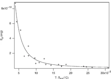
Eq. (22)) by using data given in Figures 10-12. Curve E∗_{(δT ) is plotted in Figure 16: it shows that the point}

Fig. 16.Point defect energy as a function of temperature. The solid line is the best fit to a power law (0.45 wt%, h = 20 µm).

defect energy diverges when T → TN A as δT−m with

m ≈ 2.2. This behavior was expected as the line must become stiffer and stiffer when approaching to the transi-tion temperature due to the divergence of the correlatransi-tion lengths ξkand ξ⊥ [18–20]. This point is discussed in more

detail in the next section.

5 Calculation of the line tension

5.1 Analytical results in the case K1= K36= K2

The director field and the energy of the first simple χ disclination line has already been calculated by Malet [29] under two assumptions:

1. The director remains everywhere parallel to the plates limiting the sample.

2. The splay and bend elastic constants are equal: K = K1= K3, but may be different from the twist constant

K2.

In that case, calculations may be done analytically and lead to the following expression for the angle φ between the director and the x axis:

φ(x, z) = 1 2arctan · coth µ πx h r K2 K ¶ tan µ πz h ¶¸ +πz 2h + π 2(E(x) + 1) − θ, (23)

where z is the coordinate perpendicular to the surfaces located at z = ±h/2, θ the angle between the line and the anchoring direction, and E(x) the Heaviside function.

As for the line energy, it is given by E1= π 4 p K2K · ln µ h 4πrc r K2 K ¶ +2C π ¸ +Ec, (24)

where C = 0.916 is the Catalan constant, rc the core

ra-dius, and Ec the core energy.

much simplified and must be improved, both by taking into account distortions of the director field out of the plane, and more importantly, by including the strong di-vergence of the bend elastic constant K3 close to TN A as

can be seen in Figure 15.

For that reason, we calculated the line energy numer-ically. Our results are presented in the next subsection.

5.2 Numerical calculation in the general case K16= K3 6= K2

To do the calculations, we used a tensorial form of the free energy. Note from now on that this formulation eliminates all the problems associated with the discontinuity of the director field on the cut surface of the Volterra process. In addition, it allows us to calculate the core energy. Let us denote by Qij the quadrupolar order parameter. In the

uniaxial approximation, valid for a long-pitch cholesteric, Qij is given by Qij= Q µ ninj− 1 3δij ¶ , (25)

where ~n is the director. The free energy contains two terms. The Landau energy of expression

fL= A 2QijQji− B 3QijQjkQki+ C 4(QijQji) 2 (26) with A = A0(T − TN A) in the mean-field approximation,

and a Ginzburg term taking into account the spatial vari-ations of the director field:

fG= L 1 2 Qjk,iQjk,i+ L2 2 Qij,iQkj,k+ L3 4 QijQkl,iQkl,j −2L1q²_ijkQ_ilQ_jl,k+ L3q²_ijkQ_ilQ_lmQ_jm,k. (27)

One can verify that fG, not only contains the

Frank-Oseen elastic energy, with the correspondence K1= (2L1+ L2)Q 2 − L3Q 3 /3, K2= 2L1Q 2 − L3Q 3 /3, (28) K3= (2L1+ L2)Q 2 + 2L3Q 3 /3,

but includes additional terms in ∇Q which become rele-vant near the core of the defect (where the Frank-Oseen elastic energy fails).

In practice, parameters A, B, and C have been mea-sured for 8CB: A = 0.18 × 107 erg/cm3 K−1_{, B = 2.3 ×} 107 erg/cm3 , and C = 5.2 × 107 erg/cm3 [30]. As a conse-quence, one can calculate from these data the value of Q which minimizes the Landau energy (26) for a given tem-perature. As we know the elastic constants (see Fig. 15),

we can also calculate from equation (27) the stiffness con-stants L1, L2, and L3. These values of the parameters will

be used in the numerics to calculate the defect energy as a function of θ at the temperature chosen.

Let us now detail the numerics. In order to calculate the director field around the defect and its energy as a function of θ, we wrote a program in Fortran. To simplify, we assumed that the temperature was constant and we neglected the thickness gradient. This imposed to choose the pitch equal to 4h in order that the nematic and the cholesteric phases have the same energy on both sides of the defect. Simulations were performed in 2D, in the plane (x, z), because the configuration is translationally invari-ant along y. The starting point was a configuration topo-logically compatible with a simple χ line making an angle θ with the anchoring direction. The corresponding Qij

-field was calculated by using the Malet formula (23) and the definition of Qij given in equation (25). This field is

then relaxed to equilibrium corresponding to the minimum energy according to the evolution equation:

Qij(x, z, t + 1) = Qij(x, z, t) − α

∂E1

∂Qij(x, z), (29)

where E1 =P_x,zf_L(x, z) + f_G(x, z) is the total energy.

Note that Qij(t = 0) corresponds to Malet configuration,

while α is a time step which must be chosen sufficiently small to allow convergence. In practice, the total energy E1was discretized before to be minimized as a function of

Qij(x, z). This explains why it is not a functional

deriva-tive with respect to Qij which enters into equation (29),

but only a simple partial derivative with respect to Qij.

Calculations were performed using a square grid of 51×51 points corresponding in the real space to a sample section of size 20 × 20 µm. This corresponds to a mesh size of 4000 ˚A much larger than the real core radius of the de-fect, expected to be of the order of a few tens ˚A [17]. For this reason, it was possible to reduce the parameters A, B, C by a factor 400 without changing significantly the calcu-lated energy and the director field configuration. Indeed, this renormalization is equivalent to increase the core size by a factor√400 = 20, the latter scaling likepL/A. This does not change significantly the calculated energy as the corresponding core size remains smaller than the mesh. On the other hand, there is a big advantage to renormalize the Landau coefficients because this allows us to increase the time step α by the same factor (×400) unless the code diverges. Hence, much faster computations can be per-formed. In practice, we consider that the configuration is at equilibrium when its energy E1is constant within 10−4

in relative value. The value of E1 obtained in this way is

the line energy upon condition that the energy density of the nematic phase (equal to that of the cholesteric phase) is set to zero, which we imposed in our calculations.

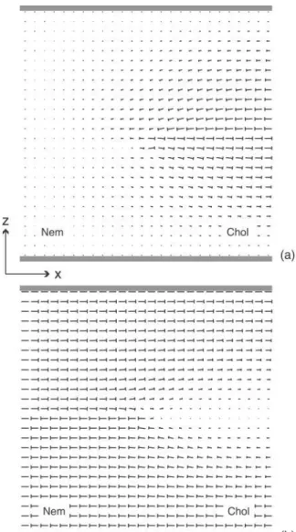
Two examples of director fields calculated numerically at δT = 0.03◦_{C are drawn in Figure 17 by using the}

classi-cal “nail” representation. As we could expect, the director exits the plane (x, y), in contradiction with Malet assump-tions assuming a planar configuration. More important is that the main director field distortions are of “splay-twist”

Fig. 17. Director fields obtained after minimizing the total energy when θ = 0 (a) and θ = π/2 (b) (δT = 0.03◦_{C). In (a),}

the deformation along the x direction is mainly of splay type, whereas in (b) it is rather of bend type.

type in the first configuration (a) (θ = 0) and of “bend-twist” type in the other (b) (θ = π/2). Because K3> K1,

we naturally predict that E1(π/2) > E1(0). This point was

confirmed numerically as shown in Figure 18a, where we see that the larger K3/K1, the larger E1(π/2)/E1(0) (we

checked numerically that E1(θ) = E1(π − θ)). As a

conse-quence the curves flatten when the temperature increases (the anisotropy K3/K1 decreases), to become almost

in-dependent of θ far from the transition temperature to the smectic phase, in agreement with Malet calculations. In order to test our program, we also ran the simulation at δT = 2◦_{C. At this temperature, K}

1 ≈ K3 according to

Figure 15, so that Malet calculations are applicable. We obtained in this case E1 = 2.5 × 10−6dyn independently

of angle θ (within ±1%) in agreement with Malet pre-dictions. This value is also reasonable in order of magni-tude. Indeed, it corresponds to that we would obtain from equation (24) by taking rc ∼ 15 ˚A and a core energy Ec

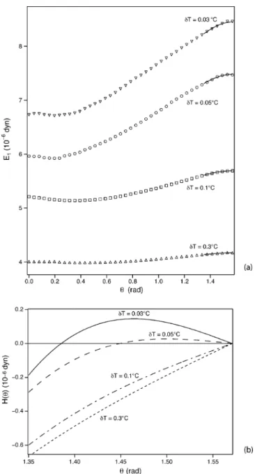
Fig. 18. Energy E1 and function H as a function of angle θ

between the line and the anchoring direction.

counting for 10% of the total energy (which is generally admitted for disclination lines [17]).

The next step was to determine whether the line desta-bilizes and, if so, for which angles. To answer this question, we fitted each curve over an angular window of twenty degrees about its maximum at θ = π/2 to a law of type

y = a+b(π/2−θ)2

+c(π/2−θ)4

. From each fit (correspond-ing to the portion of curve drawn in solid line in Fig. 18a) we calculated the function H(θ) defined in equation (8). These new curves are shown in Figure 18b. We observe that the two curves calculated at δT = 0.03◦_{C and 0.05}◦_C

pass through positive maxima for angles θm = 84◦ and

86◦_{, and vanish for angles θ}

0= 79◦ and 83◦, respectively.

By contrast, the two other curves calculated at higher tem-peratures are always negative. These results demonstrate

Finally, let us estimate the typical size ξ of a point de-fect between a “zig” and a “zag”. By taking E∗_{∼ ξE}

1(θ0)

and by using the values of E∗ _{given in Figure 16, we find}

that ξ ∼ 40 nm at δT = 0.03◦_{C. This value is}

compara-ble to the smectic correlation lengths measured by X-rays at this temperature [24]: ξ⊥ ≈ 20 nm, ξk ≈ 200 nm. This

result is not surprising as the line must become very stiff over distances of the order of, or smaller than, the smectic correlation lengths.

6 Conclusion

In conclusion, we have described a new method to measure the pitch divergence in the close vicinity of a cholesteric-smectic A phase transition. Note that this method could be used likewise to measure the pitch divergence in cholesterics that possess a compensation point where the twist changes sign. In these materials, we should not ob-serve any zigzag instability of the χ lines as K3 has no

reason to diverge. Indeed, the zigzag instability is due to the divergence of the elastic constant K3 close to the

smectic phase, as we have shown experimentally and nu-merically in this article. We must nevertheless confess that our numerics is incomplete as it was performed at constant temperature. One improvement would be to introduce the temperature gradient but we are not sure this would bring any significant new insight to our understanding of the problem.

Much more interesting from our point of view would be to study the dynamics of the lines. This could be done by moving the sample in the temperature gradient at a constant velocity. Measuring the position of the line with respect to the smectic front as a function of the imposed velocity should allow us to measure its mobility as a func-tion of temperature, and could give valuable informafunc-tion about the divergence of the rotational viscosity γ1 close

to the smectic phase.

We thank J. Baudry for his help for writing the Fortran pro-gram used in this article.

References

1. P. Oswald, F. Melo, C. Germain, J. Phys. (Paris) 50, 3527 (1989).

2. P. Nozi`eres, Shape and growth of crystals, in Solid Far From Equilibrium, Beg Rohu Lectures, edited by C. Go-dreche (Cambridge University Press, Cambridge, 1992). 3. C. Herring, Phys. Rev. 82, 87 (1951).

4. M. Flytzani-Stephanopoulos, L.D. Schmidt, Prog. Surf. Sci. 9, 83 (1979).

5. D. Knoppik, F.-P. Penningsfeld, J. Cryst. Growth 37, 69 (1977).

6. J.C. Heyraud, J.J. M´etois, J. Cryst. Growth 84, 503 (1987).

7. D.G. Vlachos, L.D. Schmidt, R. Aris, Phys. Rev. B 47, 4896 (1993).

8. F. Melo, P. Oswald, Ann. Chim. France 16, 167 (1991). 9. F. Melo, P. Oswald, Phys. Rev. Lett. 64, 167 (1990). 10. J. Friedel, Dislocations (Pergamon Press, Oxford, 1967). 11. Orsay Liquid Crystal Group, Phys. Lett. A 28, 687 (1969). 12. Groupe des Cristaux Liquides d’Orsay, J. Phys. (Paris)

Colloq. 30, C4-38 (1969).

13. M. Kl´eman, J. Friedel, J. Phys. (Paris) Colloq. 30, C4-43 (1969).

14. M. Miha¨ılovic, P. Oswald, J. Phys. (Paris) 49, 1467 (1988). 15. Y. Galerne, L. Liebert, Phys. Rev. Lett. 55, 2449 (1985). 16. C. Chevallard, M. Clerc, P. Coullet, J.-M. Gilli, Eur. Phys.

J. E 1, 179 (2000).

17. P. Oswald, P. Pieranski, Nematic and Cholesteric Liquid Crystals, in the Liquid Crystals Book Series (Taylor & Francis, 2005) p. 438.

18. R.S. Pindak, C.C. Huang, J.T. Ho, Phys. Rev. Lett. 32, 43 (1974).

19. C.C. Huang, R.S. Pindak, J.T. Ho, Phys. Lett. A 47, 263 (1974).

20. Shu-Hsia Chen, J.J. Wu, Mol. Cryst. Liq. Cryst. 87, 197 (1982).

21. P. Oswald, M. Moulin, P. Metz, J.C. G´eminard, P. Sotta, L. Sallen, J. Phys. III 3, 1891 (1993).

22. R. Alben, Mol. Cryst. Liq. Cryst. 20, 231 (1972). 23. F. J¨ahnig, F. Brochard, J. Phys. (Paris) 35, 231 (1972). 24. D. Davidov, C.R. Safinya, K. Kaplan, S.S. Dana, R.

Schaetzing, R.J. Birgeneau, J.D. Litster, Phys. Rev. B 19, 1657 (1979).

25. J. Thoen, H. Marynissen, W. Van Dael, Phys. Rev. A 26, 2886 (1982).

26. C.W. Garland, G. Nounesis, Phys. Rev. E 49, 2964 (1994). 27. N.V. Madhusudana, R. Pratibha, Mol. Cryst. Liq. Cryst.

89, 249 (1982).

28. S. DasGupta, S.K. Roy, Phys. Lett. A 288, 323 (2001). 29. G. Malet, Structure et dynamique des lignes de Grandjean

dans les cristaux liquides cholest´eriques `a grands pas, D.Sc. Thesis, Universit´e des Sciences et Techniques du Langue-doc, Montpellier (1981).