HAL Id: ensl-00248419
https://hal-ens-lyon.archives-ouvertes.fr/ensl-00248419v3
Submitted on 14 Feb 2008
HAL is a multi-disciplinary open access archive for the deposit and dissemination of sci-entific research documents, whether they are pub-lished or not. The documents may come from teaching and research institutions in France or abroad, or from public or private research centers.
L’archive ouverte pluridisciplinaire HAL, est destinée au dépôt et à la diffusion de documents scientifiques de niveau recherche, publiés ou non, émanant des établissements d’enseignement et de recherche français ou étrangers, des laboratoires publics ou privés.
Pictures worth a thousand tiles, a geometrical
programming language for self-assembly
Florent Becker
To cite this version:
Florent Becker. Pictures worth a thousand tiles, a geometrical programming language for self-assembly. Theoretical Computer Science, Elsevier, 2009, 410 (16), pp.1495-1515. �10.1016/j.tcs.2008.12.011�. �ensl-00248419v3�
Pictures worth a thousand tiles, a geometrical programming
language for self-assembly
∗Florent Becker
LIP — ENS LYON — UMR CNRS 5668 46 allee d’Italie 69364 Lyon cedex France [email protected] February 14, 2008 Abstract
We present a novel way to design self-assembling systems using a notion of signal (or ray) akin to what is used in analyzing the behavior of cellular automata. This allows purely geometrical constructions, with a smaller specification and easier analysis. We show how to design a system of signals for a given set of shapes, and how to transform these signals into a set of tiles which self-assemble into the desired shapes.
We show how to use this technique on three examples : squares (with optimal assembly time and a small number of tiles), general polygons, and a quasi periodic pattern : Robinson tiling.
1
Introduction
Self-assembly is the very common phenomenon of spontaneous emergence of shape (and thus func-tion) through accretion of small basic components. It can be observed at the microscopic scale through the formation of crystals and quasi-crystals, in the formation of coral reefs. It is also a major challenge for nano-technology: assembly of nano-components through external means is a delicate and costly process, and replacing this “manual” assembly process with self-assembly could lead to tremendous improvement in speed. This is witnessed by the experimental results of Rothemund, Winfree et al. in [Rot01], where they actually implement self-assemblin tile-sets or in [Rot05], for some more implementations of the closely related technique of self-folding DNA strands.
Since Winfree [WLWS98, Win95], there has been an ongoing interest in a theoretical model of this phenomenon, self-assembling tilings. This model comes from the tradition of theoretical computer science, and draws its roots in Wang tilings. As in Wang tilings, the basic components are Wang tiles, that is unit squares with colors on their edges. By adding glues to the edges of these tiles, one can create self-assembly: given a finite set of tile types, put an infinite number of copies of each tile type in a “pot”, watch them stick to each other, and see what is (are) the shape(s) of the resulting aggregates.
∗
This model has led to a number of results and techniques, which have allowed for the assembly of arbitrary computable shapes [WYS96], with very few tiles [ACG+02], in the presence of errors
[WB03], and so on [SW04a, Win06].
In this paper, we present a geometrical approach to a more compact and legible presentation of self assembling tile systems. We give a geometric programming language based on straight line signals which abstracts the process of self-assembly. This simple language is not too restrictive, and can model most of the constructions of self-assembly from the literature.
Signal systems are a classic device in the study of Cellular Automata and computation. They have led to a variety of papers, such as [MT99] in the context of CAs or [DL05] for computation with purely abstract signals. Their importation in the world of self-assembly is not immediate, since in self-assembly, space and time are more entangled than they are in classic models. We need to introduce a Time Consistency condition in order to ensure that a diagram made of signals actually makes sense in terms of self-assembly.
With this new formalism, we are able to give three constructions. The first one is for squares; it works in optimal time with a constant number of tiles, thus 32 times faster than in [BRR06]. The second is a way to build any convex polygon, and shows a little refinement of the programming language, as it uses weak links in self-assembly. This construction allows, with a small number of tiles, to assemble polygons with an arbitrary good resolution. This kind of constructions allows self-assembly to get rid of “aliasing” problems. These problems are very common in the constructions of the literature, and they are genarally silently ignored. In fact, the resource “resolution” is the one that is used to implement all the nice tricks of self-assembly, be it Turing computation or fault tolerance. The framework we use for polygons could probably be adapted to other constructions to smoothen their output.
Last, we show a construction of Robinson tilings. This is the first quasiperiodic construction in self-assembly. It also shows how to deal with infinite output within our paradigm. These infinite outputs have never been dealt with in a systematic manner, with definitions in [PWR04] being implicit. This is also an example of a local computation resulting in a strictly quasi-periodic pattern where the computation is local only and yet does not rely on trial and error. The use of our Time Consistency condition to keep a global synchronization is crucial.
2
Self assembling tilings
Definition 1 (The model of self-assembly). A seeded tile system is a 5-tuple T =< T, t0, τ, g, P >.
Each of these variables is defined in the following.
• The set of tiles. T is a finite set of tiles. Each of these tiles is an oriented1 unit square with
the north, east, south and west edges labeled from some alphabet Σ of glues (or colors). For each t ∈ T , the labels of its four edges are canonically denoted σN(t), σE(t), σS(t) and σW(t).
• The seed. t0 ∈ T is a particular tile known as the seed.
• The temperature. τ is a positive integer called the temperature. In this paper, τ = 2.
1Whether tiles are oriented or not does not change the problem much, since the orientation of each side of a tile
can be encoded in its color. This way, the rotation of the tiles can be prevented. Still, it is clearer to reason about oriented tiles than unoriented ones
• The strength function. The function g goes from Σ to N.The value g(α) is called the strength of α. There is a special glue, null with g(null) = 0. The attraction between two glues is given by the function g2(x, y) = δyx· g(x). That is, the attraction between two different glues is null,
and the attraction between two identical glues is given by g.
T -transitions. A configuration is a map from Z2 to (T ∪ {empty}), where the tile empty is
the one having in its four sides the glue null. Let A and B be two configurations. Suppose that there exist t ∈ T and (x, y) ∈ Z2 such that A = B except for (x, y) with A(x, y) = empty and
B(x, y) = t. If also
g2(σW(A(x + 1, y), σE(A(x, y)) + g2(σE(A(x − 1, y)), σW(A(x, y)))+
g2(σS(A(x, y + 1)), σN(A(x, y))) + g2(σN(A(x, y − 1)), σS(A(x, y))) ≥ τ
then we say that the position (x, y) is attachable in A, and we write A →t@(x,y) B. We write A →T B when such a t, (x, y) exist. Informally, this means that B can be obtained from A by
adding a tile t in such a way that the total strength of the interaction between A and t is at least τ . Let →∗T denote the transitive closure of →T.
Derived supertiles. The seed configuration, Γt0, is the one that satisfies Γt0(0, 0) = t0 and,
for all (x, y) 6= (0, 0), Γt0(x, y) = empty. The derived supertiles of the tile system T are those
configurations X such that Γt0 →
∗
T X. Final supertiles are those from which no further transition
can be made.
Production of shapes. A shape is a 4-connected finite subset of Z2. The shape of a derived supertile A will be denoted by [A] and corresponds to {(x, y) ∈ Z2 : A(x, y) 6= empty}. The set of shapes of final supertiles is the set of final production; it is the output of the tile system.
Direction of a tile. The direction of a transition is the direction in which it has extended the pattern. If t consists of adding a tile at z = (x, y), then the direction of t depends on the neighbours of z which are in the pattern before t is added. If z only has one neighbour, then the direction of t is the opposite of the direction of that neighbour (if the neighbour is (x, y − 1), then t has direction N). Similarly, when there are two neighbours, if they are, say, the western and southern ones, then t is NE. When z has more than two earlier neighbours, or two opposite neighbours, we say that it has no direction.
From now on, we will consider only temperature 2 self-assembling system. From a chemical point of view, the lower the temperature is, the simpler it is to implement the system. In practice, temperature 1 is not powerful enough from a combinatorial point of view to allow interesting constructions, and temperature 3 is not chemically feasible. Moreover, temperature 2 is all we need for translating signals into tiles. This means that all our constructions work at higher temperatures by scaling the glue strengths appropriately2.
The RC condition Consider a temperature 2 self-assembling system. If in a derived supertile, there is exactly one tile with a strength 2 glue on its northern (respectively southern) edge per row, and one with a strength 2 glue on its eastern (respectively western) edge per column, we say that the supertile is RC (Row-Column). Thus, for a row north (respectively north) of the seed, the first tile to be put is the one with a strength 2 glue on its southern side (respectively northern). Likewise for columns.
2When the temperature is odd, one has to favour one of the axis by rounding strengths on that axis up, and down
The direction of the transitions which lead to an RC supertile can be determined by looking at the position of the tile with respect to the first tile of its row and column. For example, if the transition happens to the south of the first tile in the column, and to the east of the first tile of the line, then the transition has a direction SE .
Self-assembling systems can simulate cellular automata (and hence Turing machines) in a RC fashion. If the stopping state of the automaton is taken to break the RC-ness of the production, then it is undecidable whether the system is RC. Therefore, this RC condition is undecidable in general.
3
The peculiarities of self-assembly
Self-assembling tilings represent a kind of compromise between two classical models: Wang tilings and cellular automata.
In Wang tilings, the notion of time is totally absent from the model: tilings exist (or not), but one does not build them. In that model, a signal is made by local constraints. There is no notion of propagation per se, the signal exists everywhere at once.
In cellular automata, a signal has a velocity, and it goes from point A at time t to point B at time t0. t, t0, A and B are constrained by the speed of light, but still, time and space are nicely orthogonal.
In a self-assembling system, things are more difficult, as time and space are entangled. In a production, each cell of the plane has exactly one time associated with it, the time at which it was attached in the derivation of the production. Also, signals in self-assembly need a medium to propagate and interfere.
The first problem with signals in self-assembly is that each cell can only change state once, from empty to full. This means that when some signals must cross somewhere, they have to arrive there at the same time or one of them will be blocked by the other one. This can be especially painful when one tries to combine several signal schemes. In cellular automata, it is enough to take the cartesian product of automata. In self-assembly, it is not so, as when two signals cross spatially, they have to also be synchronized.
Another subtlety concerns the possible slopes of the signals. The spatial slope of a signal is also an image of the order in which the tiles have been attached. For example, in order to propagate information from the South-West to the North-East, it is crucial that in each line, the tiles are attached from left to right, and in each column from down upwards: a tile can only depend on its neighbours if they were attached before itself. If we want to draw a picture with signals, the order in which we draw it determines what it can look like.
Lastly, self-assembly is an asynchronous process, in which there are two sources of non-determinism. The first source comes from the choices to be made when putting a tile at a given place. The second is the choice at each time of where the next tile will be put. This non-determinism is more difficult to take in account, as it demands a global analysis of the assembly process : one can have global non-determinism even in the presence of local determinism.
In the self-assembling systems of the literature, these difficulties are solved with the help of the RC condition. We will use this same RC condition for our constructions, in a form adapted with continuous signals.
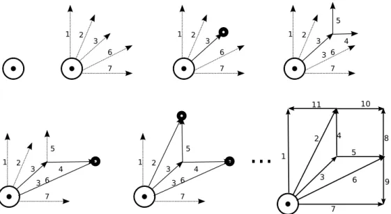
Figure 1: A self-assembling system E for assembling a square, presented through a 7 × 7 production
(a) The signals. (b) The order of con-struction.
Figure 2: An abstract view of the assembly of a square
4
Signals systems
The idea of signals system comes from the observation of how most tile-set are actually conceived. Let us take a simple problem: we want to assemble the set of all squares, and we want the assembly to have an optimal speed. Our exact measure of speed, defined in [BRR06] and [SW04b] is not crucial for this developement. Let us simplify the problem by only considering squares of even size. We count size as the distance between the center of the tiles; thus, those squares have an odd number of tiles. This oddity allows us to use actual distances when we will work with signals later. The tileset E depicted on figure 1 is an example of what one can do. It is not the most economic in terms of number of tiles, but it works in optimal time, and nicely shows the essential features of signal interactions.
Figure 1 does not show how we actually think about this tile-set. We have a much more abstract view of it, like figure 2(a). Figure 2(a) can in fact be turned into a formal definition of a geometric programming language. Programs in that language can in turn be transformed into a self assembling system.
In figure 2(a), what we see is the flow of information in the shape as it is being assembled. In substance, it states that what we do in order to build a square is the following: we draw a diagonal upto the point that will be the center of the square; Then we transmit the information that the assembly should stop by sending signals to the middle of the edges opposite the source, which we find as the intersection of lines 2 and 4; Then, it is possible to finish the square.
which the tiles are put. This is not realistic in the context of DNA self-assembly which is a parallel and random process, and neither does it correspond to the model of self-assembling tilings. In order to implement such a construction scenario in a self assembling system, we need to specify the dependencies, and to account for them in the design of the set of tiles. This gives a drawing like figure 2(b).
This figure reads as follows. First, notice that all the signals no longer have the same status: 2 and 6 are now privileged. The small arrows on the signals 2 and 6 are their expansion direction, respectively N and E. What this means is that at a given time, the construction can only go as far north as 2 has advanced, and as far east as 6 has advanced. In the self assembling system E , this is implemented by having the first tile of each row be “on” signal 2, and all first tile of each column on signal 6. Remember that these tiles are necessarily the ones with strength 2 glues. Thus, the signals 2 and 6 control the expansion of the construction in their expansion direction. They cut the square into 3 regions, each with a diagonal expansion direction. For instance, the central region has a NE expansion direction, which means that a tile in that region is put after its southern and western neighbors. Hence, this region grows in the NE direction. With these constraints, the transmission of information takes place as wanted, as the signal 2 has to wait for 4 further east (likewise for 6 and 5).
4.1 The visual syntax of Signal Systems
The conjunction of these two drawings is what we will define more formally as an expanding signal system (ESS), from which we are going to define our tile systems. ESS live in the plane R2equipped with the distance l1 or Manhattan norm: |(a, b)| = |a| + |b|. Given a suitable ESS, we will be able
to automate the design of the tiles, making the design more intuitive, and the proofs easier. Definition 2 (Expanding signal system). An expanding signal system is given by a finite set of region types R, a finite set S of signal types, and a finite set C of collision types .
• A region type is defined by its name. There is a special region called the exterior. • A signal type is given by
– a vector s ∈ Z2, the slope,
– a potential expansion direction d ∈ {H, V, O} (for Horizontal, Vertical and nOne). Signal types with a horizontal slope cannot be V, and signals with a vertical slope cannot be H. – two adjacent regions, one on the left and one on the right.
– a bit, defining the signal as either one time or repetitive.
• A collision type c is made of two set of signal types, c− is the set of its incoming signals, and c+ is the set of its outging signals. A collision has to be consistent. By consistent, we mean the following: let c be a collision, for s ∈ c+∪ c−, the subjective slope of s as seen by
c is slope(s) if s ∈ c+, and −slope(s) if s ∈ c−. Its signal enumeration is the function from Z/|c|Z to c+∪ c− defined by enumerating the signals of c+∪ c− in the order of their subjective slope (in counter-clockwise order). A collision is consistent if, in its signal enumeration, for any i ∈ Z/|c|Z, the left region of the signal i is the same as the right region of the signal i + 1. • C contains a special collision type, the source . For the source, we have: − = ∅.
Figure 3: The signals system for squares. Up, the signals with their slope vectors. H signals have an horizontal triangle on them, and V signals a vertical triangle. All signals are repetitive. Down, the collisions. Signal names are the numbers, and region names are the letters on the side of the signals.
Symetrically to , a signal system can have end collisions, for which c+ = ∅. We will see that these collision are essential in order to produce finite drawings.
4.2 Signal systems in action
Definition 3 (Sketch). A sketch on a set L on a is a quadruple (P,S,H,F) with P a set of points, S a set of line segments, H a set of half-lines and F a set of faces on the plane such that:
• The end-points of all segments and half-lines are exactly the points P • Faces of the sketch are delimited by the lines of the sketch.
Each element of P , S, H and F has a label in L.
For a sketch c, we note c(x, y) for the element of c that contains the point (x, y).
Each signal system defines a grammar of sketches. Instead of strings of symbols, our grammar uses symbols on elements of a sketch. The productions of this grammar are called non-complete drawings, and its terminal productions are called complete drawings (or simply drawings).
The set of symbols we use are the collision types, signals types and region types from S, all of them terminal. We also have a non-terminal symbol ¯s for each signal type s and one (¯c) for each collision type c. Points are labeled by collision types, lines by signal types, and faces by region type. Henceforth, we call the points of a drawing, signals its lines, and the faces regions.
The derivation rules for a given signal system are the following: Initial production ¯ at (0, 0) is the initial production of the grammar
Region To any active whose edges all have a terminal symbol, attribute the unique region type that is compatible with the signals types of the edges.
Collision for any set of non-terminal signals S concurring to an integer point p such that there is a collision type c with c− = S, add a collision at p with type ¯c. Then replace each of the signals ¯s with a segment s stopping at p. This rule only applies if the resulting signals don’t intersect any other signal.
Outgoing signals for any point p with collision type ¯c, add
• a half-line from p with slope s(t) and with signal type ¯t for each repetitive signal t ∈ c+ • a segment from p to p + s(t) with signal type ¯t for each one-time signal type in c+ • Change the type of the collision to c.
These rules imply in particular that no signals cross elsewhere than at a collision in a complete drawing.
We say that a signals system is correct if for any non-complete drawing, there is a complete drawing that contains it. This essentially means that signals don’t intersect at non-integer points, and only as prescribed by the collisions. Both of these conditions are of course undecidable for general signal systems, but they are more clear and natural to prove than the minute details of the behaviour of a self-assembling tile-set. They correspond to the halting question for programs in classical languages: their indecidability is a fundamental fact of computation, but we still prefer
Figure 4: An example derivation of a square by our ESS. Non-terminal collisions are represented by a circle, and non-terminal signals have dangling ends.
to analyse code written in our favorite language rather than in raw machine instructions of Turing states.
If we remove the integer-coordinates condition we get something akin to signal systems `a la Durand-Lose [DL05]. We would then have to deal with accumulation points, which is in general impossible with a finite tile-set.
A collision (or signal) c0is said to depend on a collision c (or signal) in a drawing if there is a path from c to c0 by following signals in their directions. In particular, all collisions and signals depend on , and if an element e0 depend on another one e, then any non-complete drawing containing e0 contains e. Intuitively, this means that e0 possesses information on e.
4.3 Are Space and Time compatible? Time Consistency
Signal drawings correspond to figure 2(a) in the case of squares: they don’t include information about the directions of expansion of the various parts of the pattern. We have to check that such a drawing can actually be drawn locally while creating its own support. Even if the depndencies don’t have a cycle, there might be conflicts or deadlocks between signals, since they also interact through the existence of parts of the drawing being made. In self-assembly, one tackles these problems by using RC constructions. Thanks to the RC condition, one can determine the flow of time in a production without looking at its actual history. Similarily, for signal systems, we introduce a continuous version of the RC condition, Time Consistency. It gives us, for each part of a drawing, a local expansion direction or the “local flow of time”.
We determine these directions thanks to the position of the seed and to the expansion directions of the signals. We will cut the drawing into provinces to which we attribute a direction. If this partition is correct, then the drawing is Time Consistent, and we have our directions.
Once the signal system is compiled into a self assembling tile system, the direction of the province will be the direction of the tiles.
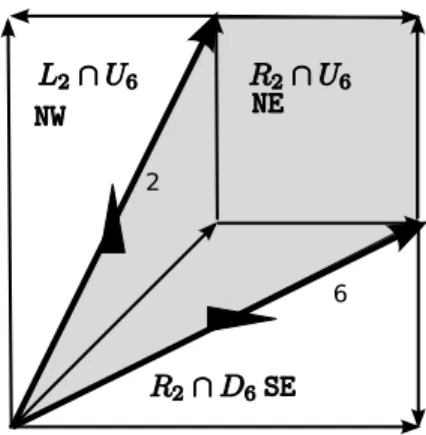
Figure 5: Provinces, in the case of the square
We define the provinces as follows. Let s = ((x, y)(x0, y0)) be a segment bearing a signal with expansion direction V . We define for this segment 2 regions of the plane:
• Ls is the left half of the horizontal band containing s, i.e. Ls = {(a, b) : min(y, y0) ≤ b <
max(y, y0) ∧ a < x + bxy00−x−y}
• Rsis the right half of that band, i.e. Rs= {(a, b)|min(y, y0) ≤ b < max(y, y0)∧a > x+bx
0−x
y0−y}
Likewise, if s has a H expansion direction, then we define the associated regions as follows: • Us is the upper part of the vertical band containing s: Us = {(a, b) : min(x, x0) ≤ a <
max(x, x0) and b < y + axy00−y−x}
• Ds is the lower part of the same band: Ds = {(a, b) : min(x, x0) ≤ b < max(x, x0) and b >
y + ayx00−y−x}
A province is the intersection of a Lsand Rs. We attribute to each province a direction according
to the following table:
∩ Us Ds
Rs NE SE
Ls NW SW
Definition 4. A drawing is Time Consistent if the following conditions are met: • The provinces form a partition of the domain of the drawing.
• For each signal whose type t has expansion direction O, the province p it appears in is such that the slope of t lies in the quarter plane defined by the direction of p.
5
Compiling Signals into Tiles
5.1 Discretization of sketches
Now that we have seen how to get a set of drawings from a signals system, we will show how it can be compiled into a self assembling system. First, we will define an interpretation of some self
assembling systems in terms of signals, then we will show that if a signals systems only gives RC diagrams, then there is a self assembling system that can be interpreted as this signals system. Our interpretation is faithful to the geometry, and a final production of a self assembling system is a discretization of a diagram of the interpretation.
Definition 5. A local configuration of a sketch is an intersection of that sketch with a unit square centered on an integer point.
Given a signal system S, and a set of tiles W , an interpretation function is a function which to each tile of W associates a local configuration of a labeled directed 2-dimensional sketch on S.3
We say that a pattern p on W is a concretization of a sketch c according to an interpretation function i if for any (x, y) ∈ R2, either
• (x, y) belongs to the exterior region of p and there is no tile at ([x], [y]) in p • or c(x, y) = [i(p([x], [y]))](x − [x], y − [y]),
where [x] represents x rounded to the nearest integer.
Informally, an interpretation function associates to each tile of a set a piece of a figure. When we have a pattern made with those tiles, we look at the juxtaposition of these patterns. If it is a valid sketch, then we say that the pattern is a concretization of that sketch.
5.2 The compilation
Theorem 1. Let S be a correct signal system such that any drawing of S is Time Consistent. Then there exists a self-assembling system S and an interpretation function such that the final productions of S are exactly the concretizations of the drawings of S. Moreover, we have an algorithm for finding S, and S is RC.
Note that the correctness and time consistency on the signal system are undecidable, as is deciding whether a signals system assembles at least one finite drawing.
5.2.1 Compilation algorithm
We will build a temperature 2 self assembling tile-system S. The definition of the interpretation function is implied by the construction, as we build our tiles as pieces of sketches.
Since collisions only happen at integer points and signals have rational slopes, there is only a finite number of local configurations that can happen in a drawing. Any given signals can only appear at a finite set of positions in a cell of the grid. Several signals can only cross the same cell if they are close enough to a collision.
These local configurations can be listed: there are at most 2q signals of slope p/q coming through any unit square in a drawing. From these, some are impossible: they contain region inconsistencies, signals which cross without collision, or imply that one of their neighbors itself is impossible: if two non-parallel signals share the same unit square, they must be implied in a collision nearby (at least one of them). This means that they must not cross before one of them at least reaches an integer point.
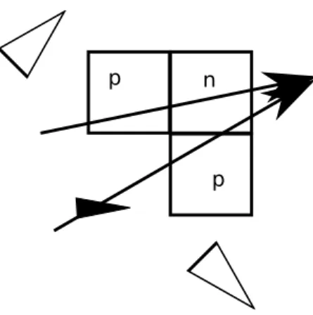
Figure 6: A tile we derive from a local configuration. Right, the color of one of the edges; this glue has strength 2 because of the V signal.
Note that one time signals are dealt with in the process: they may only pass through integer points a fixed number of times, and can be made to change color each time. Then their extremal local configurations can be removed, as they contain a signal stopping without collision, which cannot happen.
One enumerates these possible configurations one adds a tile for each of them. The color of the glues between two tiles is the configuration of the corresponding edge (taken as a closed segment). The strength of the glues depends on the type of the signal which cross it. A vertical edge has a strength 2 glue if it is crossed by a H signal, and an horizontal edge if it is crossed by a V signal.
Note that the above algorithm, applied to an arbitrary ESS, can yield quite a big tileset (ex-ponential at most). This can be necessary in some cases, with lots of parallel but different signals running side by side, but is often a waste. However, if one can prove that no local configuration of a drawing contains both a collision and a signal not involved in that collision, then the tile-set can be made to have size O(sq), with s the size of the ESS and q the gcd of the slopes. In fact, in that case, we can optimize the algorithm by stating that two signals in a local configuration must be involved in a common collision. Determining the legal local configurations amounts to starting with each collision and looking outwards how the signals split into different cells. This also makes the algorithm work in O(sq). This optimization applies to all the ESS we present in this paper. 5.2.2 Proof of the construction
We establish the correctness of this self-assembling system by showing that any derived supertile can be completed into a concretization of a complete drawing, and that any finite drawing can be reached as a final production.
Correction
Lemma 1. For any derived supertile c of the system constructed above, there is a drawing d such that c can be completed as a configuration of a Wang tile set into a concretization of d. That is, ∃c0 ∈ SZ2, c ⊂ c0 and c0 is a concretization of d.
Proof. By induction.
Figure 7: Local choices in the case when there is no collision in the cell: the two previous tiles bring enough information to put the next one. The hollow triangles represent the directions of the provinces.
Now consider c1 →t@(x,y) c2, and let c0 be a concretization which contains c1. If in c0, the tile
at (x, y) does not contain a collision, then there is only one type of tile that can be added at (x, y), and that is t. This comes from the Time Consistency condition, and how it is translated into the RC condition.
If we only have O signals on a tile, then this tile will be attached to two neighbours, those corresponding to the direction of the province we are in. Because of Time Consistency, signals can only come from that same quarter-plane, so we only have one possible local configuration given the edges of the neighbours.
Consider a case with a H signal s on the tile with a positive slope. Suppose this signal marks the limit between a N E and a SE province. Then because of time consistency, all signals which get onto the same tile as s have to come from the south-west if they are higher than the signal, and from the north-west if they are lower than the signal. Only the first case is possible, and the first tile which the two signals share is one where s comes from down, and the other signal from the left. This means that this tile could only be put after its S and W neighbours. Hence, there is no choice when putting the tile at (x, y). Thus, c0 also extends c2.
If (x, y) contains a collision, then the set of tiles that can be added at (x, y) corresponds to the set of collision that are compatible with the signals seen at (x, y). By correctness, for each of these collisions, there is a drawing which contains c1 and has that collision at (x, y). Thus, all derived
supertiles can be
Conversely, take a final production, it can be completed into the concretization of a valid drawing. It covers the whole domain of that drawing, since every signal with expansion direction H or V must be complete and, because of the RC condition, any province also.
Completeness
Lemma 2. For any drawing d of S, there is a final production p of
As shown earlier, the choices for the tiles with a collision on them mimics the indeterminacy at work in that collision. By replaying the choices of the drawing when placing the tiles that bear the collision, we can control which drawing d extends a pattern. Thus, we get a
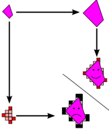
Figure 8: Discretization after scaling yields much more regular shapes than the converse
6
Assembling polygons
After squares, we tackle the more generic problem of convex polygons. Given a model convex polygon with integer coordinates, we want a tileset whose final productions are all the homothetic of this model polygon. In order to assemble a polygon with tiles, we need a discretization. Thus, we say that we assemble a polygon p ∈ R2 when we assemble the set Z2∩ p. Note that when we say that we assemble an homothetic k · p of a polygon p, we assemble a discretization of the homethetic. This means that up to rescaling, we have an arbitrarily good resolution.
The motivation to assemble the set of all homothetics of a given shape is given in [BRR06]. This allows to get rid of counters used to control the size of the production and to keep the number of tiles we use low. It also allows for more geometrical and simpler constructions, as is witnessed by our use of signal systems.
In order to assemble a polygon, we need it not to be degenerate: as it turns out, in discrete geometry, the discretizations of convex polygons, as defined above, do not have the nice properties such as connectivity which we are used to expect from them on the plane R2. Because of this,
we will at first add some restriction on the polygons in order to state our result, then we will see how to deal with these restrictions. First, we have to restrict ourselves to connectible polygons p, whose discretization is connected from a sufficiently fine resolution. A polygon p is connectible if and only if for each vertex of v of p, there exists a vertical or horizontal half-line issued from v whose intersection with p is not reduced to {v}.
Let p = (v0, . . . , vk) ∈ Nk be a polygon with vN its highest vertex (the one with the greatest y
coordinate, and vS the lowest, vW the westernmost, and vE the easternmost. We call N E quadrant
the vertices between vN and vE, and so on.
For two successive vertices z0 = (x0, y0) and z1= (x1, y1), z0∧z1is the point among {(x0, y1), (x1, y0)}
that is on the same side of the line z0z1 as p.
We call outer triangles the elements of
O = {z0, z0∧ z1, z1|z0, z1 two successive vertices of p}
and inner triangles those of
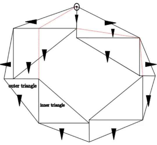
Figure 9: A (tentative) ESS for building polygons with signals
We say that a polygon is nice when none of these triangles intersect, and all of their sides have length at least 3.
6.1 A construction for the nice case
In figure 6.1, we give an example of a drawing of the ESS we will be using.
Theorem 2. For any nice polygon p, There is a self assembling system at temperature 2 which assembles the set {np}n∈N. The number of tiles in that system is O(c), the circonference of p.
A similar theorem is also true of non-nice polygons, but the proof requires some more techni-calities which we will see later.
6.1.1 ESS associated with p, first try
The associated ESS is built as shown on figure 6.1. Note that in this figure, all the “construction” points which were added have integer coordinates, as they are the intersection of vertical and horizontal lines passing by points of integer coordinates.
There is one collision type for each vertex of each triangle, inner or outer, with the collision type associated with v0 being the source. For each of these collision types, c+ and c− are simply
defined as induced by the definition of the signal types.
The two outer triangles containing are special, they will be treated last. In all the remaining of the description, read “all (outer) triangles” as “all (outer) triangles but these ones”.
There is a signal type associated with each edge of each outer and inner triangle, including the edges of p . These signals also go down, and when they are horizontal, they go towards the outside of p. The legs of these triangles are signal types of expansion direction O. The expansion directions of the hypothenuses are given in the table 1.
Within each quarter, we were able to transmit the size of the triangles from one to the next using the fact that they always shared an edge, which allowed us to have a collision starting the construction of each triangle, and a stopping signal. When one considers two adjacent triangles which do not belong to the same quarter, it is generally not so: for one of the triangles, the segment
quadrant NE SE NW SW
inner triangle V O V O
outer triangle H V H V
Table 1: Expansion directions on the hypethenuses of the triangles
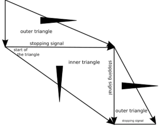
Figure 10: A closer look at three triangles in the SE quadrant
which they share is just a part of its edge. We will consider the border between the NE quarter and the SE quarter. The case of the NW and SW quarters is symmetrical. There are two possibility: either the NE triangle tN is wider than the SE , or the SE triangle tS is wider than the NE .
Let (x0, y0) be the South-West vertex of tN, (x1, y0) be the North-West vertex of tS, and (x2, y0)
be the vertex of the polygon. In the first case (represented in the East on figure 6.1 and also in figure 11), we will add in tN a O signal that will cross the line y = y0 in (x1, y0). This signal will
start from (xN, y0), the top vertex of tN. This signal takes place on a line with rational slope, so,
by the same reasoning as with the triangles, we can get a signal type for that signal. This allows us to put a collision which stops the construction of tS at (x1, y0), and carry on with the rest of
the construction.
In the second case (West in figure 6.1, and also in figure 12), there is an outer triangle of either the NE or NW quarter which intersects the line x = x1. Let t0N be that triangle, and yN the y
coordinate of its southern edge. We can send a passive signal to (yN, x1) by sending a vertical O
signal. This signal will have to cross the hypothenuse of one inner triangle. We bend slightly this hypothenuse so as to make the intersection an integer point. We can then send a passive vertical signal from that point, and a horizontal passive signal from (x0, y0) to find (x1, y0), from which we
can build tS.
Please assume for the time being that we have a construction for the two first triangles. 6.1.2 Berlin Wall
This ESS is ad hoc, and it is easy to see that the set of diagrams which it assembles are the set of the homothetics of p. It seems we hold our ESS for assembling the homothetics of p. Alas, none of these drawings is Time Consistent, as a the the Ls and Rs for s, s0 ∈ V intersect whenever s and
Figure 11: A closer look on the transmission between quadrant in the Eastern case
Figure 12: A closer look on the transmission between quadrant in the western case: the dashed line is the new signal, it bends slightly an hypothenuse to make the intersection an integer point.
Figure 13: Problematic interferences between the east and the west: when the grey part has been assembled, tiles can be put in the light rectangle, which is not included in p, because the drawing is not RC.
Figure 14: The Berlin Wall
s0 are at the same height in p, one on the Western side, and the other on the Eastern side. As a consequence, if one applies the compilation process of theorem 1, one gets a tileset which can grow shapes that are bigger than p because of interferences between the western and eastern threads. To remedy this, we need to build a Berlin Wall between East and West which prevents them from interfering.
Formally, this Berlin Wall will be presented as a set of signal types with a new expansion direction, Vertically Absorbing, with the rule that an VA signal marks a limit for any Ls or Rs.
With this addition, the diagrams are Time Consistent. This signal is implemented by tiles with a glue of strength 0 on their N and S edges. That is, one can prove an analog to theorem 1 with Absorbing signals implemented by tiles with a strength 0 glue.
The actual Berlin Wall we use is not straight, and we need some auxiliary signals and collisions to draw it, as shown on figure 14
This allows the construction to be Time Consistent, and hence gives, for any nice polygon, a tile set which assembles all the homothetics of that polygon. The exact scale one gets can be controlled
Figure 15: The construction of the largest of the two initial triangles
via the length of the first signal. This length can be controlled by tweaking the concentrations. This gives an image of p with a constant number of tiles whichever resolution we choose to have. 6.1.3 Initialization
We haven’t yet explained how we build the two triangles adjacent to the top vertex of p, and which are used as a yardstick throughout the rest of the construction. We take the one whose southern edge is the highest, say ((xt, yt)(xt, yt− h)(xt+ w, yt− h)). We use a signal type of
slope (0, −h) to draw the line (nxt, xyt)(nxt, nyt− nh). Then, the construction of the triangle
((xt, yt)(xt, yt− h)(xt+ w, yt− h)) can take place normally. Then we turn the other triangle into
a trapezoid, which we can also draw with signals.
Lemma 3. For any nice polygon p, there is an ESS with Absorbing signals whose set of drawings is {np}n∈N, and whose drawings are all Time Consistent.
Thus, by a version of theorem 1 adapted for Absorbing signals, we get theorem 2.
6.2 Coping with not-so-nice cases
6.2.1 Degenerate triangles
In the above construction, we have supposed that there was no vertical or horizontal side in p —if there was, some outer triangle would be degenerate, which is not nice. This is not a problem : if the degenerate triangle is not adjacent to the yardstick, then the construction proceeds normally by just omitting it; else, we can replace it with a rectangle.
6.2.2 Overlap of triangles
We solve the problem of overlapping triangles by replacing the conflicting triangles with quadrilat-erals. This includes the case where a triangle of the skin is not included in the polygon.
We say that an outer triangle t1 is implied in a conflict with another outer triangle t2 if t1
intersects an inner
We modify the skin in order to eliminate conflicts in the following way: we replace the outer triangles with quadrilaterals (possibly degenerate) , and we will remove the conflicts between the quadrilaterals by an operation of rollback.
Figure 16: A succesfull step of rollback
Let t = (z0, z1, z2) be an outer triangle, and z1 its right angle. Let us suppose that t is in the
NE quarter. We replace t with the quadrilateral q = (z0, z1N, zE1, z2), where z1N and z1E are two
instances of z1, which we will call the mobile vertices of q. We say that the direction of z1d is d.
The inner triangle at the south of t becomes (zE
1, z2, z3), and the inner triangle at the west becomes
(z1N, z0, z−1), which means that they will be affected by subsequent moves of zN1 or z1E during the
rollback of q. The definition of conflicts for quadrilaterals is analogous to that for triangles. Now that our quadrilaterals are ready, we repeat the following step of rollback as long as there are conflicts in the polygon: take a quadrangle q which is implied in a conflict, and is not adjacent to the top vertex of p, choose one of its mobile vertices, and move it one step in its direction, except if this would bring it onto another vertex of q. This is illustrated in figure 16. This process converges to a non-conflicting skin.
In fact, one can even assure that inner triangles as well as outer quadrangles do not intersect. Moreover, if there are degenerate quadrangles, ie quadrangles where only one of the mobile ver-tices has been moved, we can move the untouched vertex once, and the quadrangle is no longer degenerate.
We say that a polygon is amenable when the rollback process converges to a partition where the discretizations of all the pieces are connected.
Lemma 4. For any connectible convex polygon p, 5p is amenable.
Simply observe that if all the triangles have been rolled back out of 1/2 · p, there can be no more conflict.4 We need to take 5p so that 5p \ 5/2 · p contains enough integer points.
Theorem 3. For any connectible polygon p, there is a self assembling system at temperature 2 which assembles the set {5np}n∈N.
First we need to show that we can assemble any amenable polygon. For this, all we need is to show how to assemble the quadrangles we got. These quadrangles are not totally random: they have two opposite edges which are segments of the discrete grid, and one of these edges will be used as input. We call inner edge the edge between the two mobile vertices. We build such a quadrangle as follows: from the vertex of the input side which was mobile, we send a signal along the inner edge. This signal has a V expansion direction. The hypotenuse is still the same signal, but we add a diagonal O signal which stops the inner edge.
4
Figure 17: Assembly of a quadrangles
Figure 18: Robinson’s tile-set
7
Robinson tiling
The third problem we tackle is the assembly of Robinson tiling. This tiling is an example of a Wang tileset which always tiles the plane in a quasi periodic fashion, and never in a periodic fashion. It is an important theorical device, linked with Berger’s theorem. It is also the first example of self-assembly of an aperiodic tiling of the plane.
7.1 The tiling
Robinson’s tile-set is made of 6 tiles, plus their rotated counter-parts. We will give here a purely factual description of some of its features. We will not give any proof. Much more details and the proofs can be found in [AD97], an annex to [GG97].
If one decorates each of the tiles by keeping only the lines and then zooming out, the resulting figure looks like an infinite extension of figure 19.
The recursive structure of the patterns A square is a closed line as seen on figure 19 The pattern consists of interspersed squares of various sizes. We distinguish these squares by their rank rather than their size. The bumped tiles form rank 0 squares, and also the vertices of rank 1 squares. The vertices of the squares of rank (n + 1) are located at the center of the squares of size
Figure 19: A bird’s eye view of a Robinson tiling. The grey frame has direction SW
n. Each of these n-squares is contained in a n-frame, which has the same center and is twice bigger, as shown on the figure. This n-frame is the set of tiles which “depend” on that square. A rank 1 square is also a 1-frame. Each n-frame contains four n − 1-frames, whose centers are the edges of the same rank-n square. Each n squares contains a L in its center: if the size of the frame is s and the center is at (0, 0), then two of the four segments (0, 0)(0, s/2),(0, 0)(0, −s/2),(0, 0)(s/2, 0) and (0, 0)(−s/2), 0 have a line on them. We attribute a diagonal direction to each frame, the opposite of the bisector of the two segments forming the L. This way, a N E n-frame occupies the N E quarter of the n + 1-frame that contains it. Each n + 1-frame contains four n-frames, one of each direction. The parent of a n-frame is the n + 1 squares which contains it.
The patterns have a recursive structure: one gets a n + 1-frame from an n square by choosing a direction for the n + 1 square, ie the position of the L in its center. The relative position of the n + 1 frame and the n frame depends on the orientation of the n frame, as stated above. Knowing this position, one has two fill the three other quarters, the four center segments and the center of the n + 1-frame. The quarters are filled with symmetrics of the n frame, and the rest depends only on the direction of the n + 1-frame. Note that if one extends a frame of direction d in a direction other than d, the resulting pattern is not a frame.
When using this recursive procedure to get a pattern, if all the directions one chooses for the successive frames are the same, then only a quarter-plane is covered. In that case, the pattern can be completed by adding an infinite L around this quarter plane and filling the other quarter-planes with similar patterns.
North-West determinism An important property of Robinson tileset R is that it can be for-mulated as a north-west deterministic tileset: that is, one can add marks to the tiles so that given two tiles at (1, 0) and (0, −1), there is at most one matching tile that can be put at (0, 0). For more details on how to achieve this, see [PK99]. As this tileset is globally invariant under rotation by π/2, this is also verified for the other diagonal directions. This will allow us to build a great part of the patterns: as long as we have determined one tile in the column x and one in the row y, we will be able to determine the tile at (x, y) by just propagating the knowledge of the tiling using this determinacy property. Thus, our main problem will be opening new rows and new columns,
that is putting the first tile in a given row or column. This can be overcome by a precise control of where these new rows and columns are open. This can be achieved thanks to the RC condition.
7.2 Self assembly for the whole plane
We have not yet defined what it means for a self-assembling system to tile the whole plane according to a pattern. We want any point of the plane to be eventually covered by a tile. This gives us a limit tiling of the plane. Then, we color the tiles of that limit tiling and look at the resulting pattern.
First, we define limit patterns for self-assembly.
Definition 6. Let T be a self-assembling system, p a production of T and p = p0 →T p1 →T
. . . →T pn. . . be a sequence of productions such that Sn∈N[pn] = Z2, we say that the pattern
S
n∈Npn is a limit extension of p.
Definition 7 (Infallible self-assembling system). Let T be a self-assembling system, we will say that T is infallible when all its productions have at least a limit extension.
A self-assembling system is infallible when any production can be extended to cover the whole plane. This actually means that given any “fair” system for choosing where the next tile will be attached, the system will eventually cover any position in Z2. We will look at the set of tilings of
the plane generated by such systems.
The limit set LTof a self-assembling system T is the set of all the limit extensions of Γt0, the
initial configuration.
Yet, looking at limit sets is not enough: we want to give ourselves some freedom, and to be able to use a layer of computation for actually doing the assembly, and then forget it when we look at the limit set. Suppose we want to obtain a pattern that is all black with red spots on the points of the form (45x, 34y). We will need to count modulo 45 and 34. Then we need to say that all the different tiles we used for this count were actually different shades of black except when the count was 0 modulo 45 for x and 0 modulo 34 for y.
For this, we introduce a projection: let i be a function from the set of tiles to a set of colors Σ, then ¯i is defined naturally on patterns by ¯ı(t)(x, y) = i(t(x, y)).
Definition 8. Let S be a set of tilings by Σ, we will say that a self-assembling system T assembles S when T is infallible, and there is a mapping i : TT → Σ such that the set {¯ı(c)|(c) ∈ LT} is S.
In order to get this self-assembling system T , we will use an analogue of theorem 1 for infinite patterns.
Let S be an ESS. Let d be a non-complete drawing, we call terminal part of d the sketch drawn by the terminal symbols of d. A limit drawing is the pendant of a limit extension for tile system: let D = d0 ↔ d1 ↔ . . . dn. . . be a sequence of derivations of the grammar associated with S. The
limit of D is the union of the terminal parts of the dn, we call it a limit drawing of S.
We extend the notion of Time Coherent for limit extensions of drawings in a natural way. With this definition, we get the following theorem. We do not give the proof, which is similar to that of theorem 1.
Theorem 4. Let S be a correct signal system such that any limit drawing of S is Time Consistent. Then there exists a self-assembling system S and an interpretation function such that the limit productions of S are exactly the concretizations of the limit drawings of S. Moreover, we have an algorithm for finding S, and S is RC.
Figure 20: Primary frames (black) and secondary frames (grey). (0, 0) is the star
7.3 Self asssembling a Robinson Tiling
Theorem 5. There is a self-assembling system T at temperature 2 which assembles the set of Robinson’s tilings without infinite line.
This theorem might be surprising: one might think that some global information is needed in order to successfully assemble a strictly quasi-periodic pattern. This global information is in fact not present in the tiles, but in the order in which they are put, as we shall see. With that construction, backtracking is not needed.
In fact, we even get the tilings with infinite lines, but as tilings of a quarter-plane or half-plane. This corresponds to the probability 0 case of an unfair choice of region to cover.
In order to build this tile system T , we will use a two layered tile system: one layer R will contain the (Determinised) Robinson tiles, and the other layer F will cater for the details of the assembly. It is this second layer, the foundation that will make use of signals. The set of tiles of our self-assembling system is a subset of F × R. The strength function will only depend on the F component of each glue, hence we will treat F as a self-assembling system, and R as a mere Wang tileset. F will be the by-product of theorem 4.
In short, we will use F to build a hierarchy of squares corresponding to a set of increasing frames of the Robinson tiling. This allows us to cover the whole plane. We call the frames that contain the point (0, 0) primary frames, and the frame whose parent is primary secondary frames (that is, a non primary frame immediately inside a primary frame). The proper part of a primary frame is the part that is not included in the previous primary frame.
Here comes the subtlety linked to the determinization of the tile set: in order to make the tile set deterministic, in the construction of [PK99], all the n-frames facing in a given direction are not the same. Some of the colors they have depend on neighbouring tiles. Therefore, in the determinized tile-set, a n-frame is not only characterized by its direction, but also by the 4 neighbouring tiles directly outside its corners (Its corner tiles). For each of these, some colors in the n-frame state whether they are vertical arms (v), horizontal arms (h), or a cross (c).
We will need to pass this information from one primary frame to the next. It also means that not every sequence of primary frames can happen, the sequences have to be consistent: one of the corner tiles is shared by the two frames, so it has to be of the same type as seen by the two frames. This in turn limits the choice for the direction of the larger primary frame.
As Robinson’s tileset is North-West deterministic, when a tile attaches to the pattern in a diagonal direction, it cannot introduce any mistake in the pattern. Therefore, for any tile t ∈ F which does not have any strength 2 glue, we can safely put all the tiles of {t} × R are in T .
The problematic of F is to cover the plane while putting the tiles with strength 2 glues where their R component can be guessed. Note that on the diagonal of a frame in a Robinson tiling,
the tiles only depend on one neighbour. More precisely, they depend on one neighbour and the information “This tile is on the diagonal d of a frame of direction d0”, where d and d0 are the direction of the diagonal and the frame.
Note finally that for any frame, the orientation of the frame can be deduced from the type of the tile in the middle of any edge of the frame. Thus, the first tile in the proper part of a given primary frame will be in the middle of a side.
Lemma 5. There is an ESS S with Time consistent drawings, and a bijection φ between the set of Robinson tilings without infinite line and the set of the limit drawings of S such that for any drawing d,
• the signals of type V or H are located :
– on the diagonals of secondary frames of φ(d),
– or are one time signals of length 1, two per primary frame, at the middle of the edges of a primary frame; the signal type in that case depend on the orientation of the primary frame. All signals in the proper part of that same primary frame depend on the extrimity of one of these signals.
• The type of any element within the proper part of a primary frame depends reflects the ori-entation of that frame.
• the center of the secondary frames contains a collision whose type depends on the orientation of that secondary frame.
• Signals mark the central arms of each primary frame.
Before we prove this lemma, let us see why it is the key to theorem 5: suppose for a moment that we do have this signal system S and that we feed it to theorem 4. We get a self-assembling system F . To get T from F we need to select the right subset of F × R. There are four kinds of tiles in F :
• the tiles that will be attached thanks to 2 strength 1 glues, for which we can safely put all F × {t} into T
• The tiles on the diagonals of the secondary frames: for these, all the information we need is one neighbour and the type of the signal they are on: because they are on the diagonal of a frame, their neighbours are symmetrical with respect to this diagonal. Thus, one of them suffices to determine the tile. So given a tile f , the signal type it is on, and a potential neighbour on the side which has a strength 2 glue, we can select a unique tile r ∈ R and add (f, r) to T .
• The tiles in the center of the secondary frames are a special case of the previous item: their input are not symmetrical, but their missing input can be guessed from the corner type of the primary frame. Therefore, there is also a unique tile r ∈ R for which (f, r) ∈ T .
• The last case is the extremity of the one time signal. This is where the choice of the orientation of the primary frame is made. Thus, we add to T all the tiles that are compatible5 with the
5
neighbour from the previous primary frame with a strength 2 glue. The choice of which of them is actually put corresponds to the choice of the orientation of the frame, and the choice of its neighbouring corner tiles.
Proof of lemma 5. The idea for S is given on figure 21. It is to build reursively one frame of each size, with each included in the next one. What we need for this recursion is to be able, given a n-frame with some suitable collisions on its sides, to build a n + 1-frame with the same collisions.
We set a collection of signals, each parametrized by one or two direction and some extra bits. In particular, each of the signals and regions carries the orientation of the n + 1-frame which is being built.
border marks the limit of the n + 1-frame.
square allows to find the centers of the n-frames, along with diag, diag2, diag3 and diag4. The signals diag* are located on the diagonals of the secondary n-frames, and they have as parameter the orientation of the n-frame, and the orientation of the n + 1 frame. They can be made H or V by the hypothesis of lemma 5. Which of them are actually H or V depends on the relative position of the previous n-frame and the current n + 1-frame as shown on figure 21.
The signal active corner marks the beginning of the n + 1-frame. The collision that initiates it is placed depending on the type of the previous n frame; if that frame’s direction is d, then it is placed in the corner d + π/2. If such a placement is not possible because the position of active corner belongs to the previous frame (in the case of two successive frames with opposite directions), then active corner is put at the other end of the same side. This signal has as parameter the direction of the central cross of the n + 1-frame, which it passes to all the other signals. On this direction depends the type of the tiles on the cross, but also the position of the signals active corner and active middle for the next frame to be built. The possible cases are summed up on figure 22
Time consistency is proven recursively by observing that if a primary frame does not violate it, then its parent neither.
From lemma 5, we get by theorem 4 our self-assembling system F . Our remarks ensure that we can find a subset of F × R in which the choice of the R components corresponds to φ, since our H and V signals are on the diagonals of frames, and have the direction of these frames as parameters. This ensures that S is infallible and assembles the set of Robinson tilings without infinite line (theorem 5).
8
Conclusion
We have presented a graphical programming language with a compilation algorithm to self-assembling system. This geometric formalism allows to work in a continuous setting rather than in a discrete world. This lifts a great burden in both the description and the analysis of many constructions. This has allowed us to build two non-trivial example constructions, one for generic convex polygons, and one for Robinson patterns.
We have exposed this expressive framework in which most constructions of the literature can be expressed. We gave its semantics and compilation algorithm into self-assembling system. The semantics make it in general impossible to have an efficient algorithm for compilation, but a simple condition on the behaviour of the signal system allows for an efficient implementation.
Figure 21: Recursive construction for Robinson frames as an ESS. Signals with a star are one-time signals. This enforces the width 1 of the gap between the four squares. Variants of this figure occur according to the relative directions of the two primary frames which are involved.
Figure 22: The position of active corner (c) and active middle (m) depending on the orientations of the two last frames
We gave for example a simple system for assembling squares, the “hello, world!” of self-assembly. The signal formalism allows one to easily grasp the behaviour of the system and check its correctness. Moreover, it represents ther reasonning one would have made to prove the self-assembling system if we didn’t know about signal systems, but in a systematic manner.
The second example, polygons, allowed us to see that geometric construction are nicely done in this context, and that the formalism can be extended for cases when the usual assembly does not give a simple solution to the problem at hand. Note that the use of the Berlin Wall is also a novelty in self-assembling system. Thus, the need for an extension comes from a peculiarity of self-assembly itself, and not from a lack of expressiveness of signals.
The last example, Robinson tiling is the first example of a self-assembled quasi-periodic pattern. It shows how nicely the simple semantics of signal system fits in the under-explored domain of infinite constructions. The scale-free presentation of signal system is here crucial to concisely express the recursive process of construction.
8.1 Future Work
Some more work can go into the optimization of the compilation process: the size of the resulting self-assembling system can in general be quite big, but some optimization make it actually feasi-ble when we have some guarantees about the assembly process. In particular, the choice of the label of regions could be improved (be more specified) in order to lower the number of legal local configurations.
The frequent device of simulating a computation within a region of the self-assembling system is not specifically accounted for in our formalism. This allows us to see that it is not as necessary as it may seem, as none of our examples make use of it. It is also possible to simulate it by drawing a space-time diagram with signals. Still, it might be worthwhile to have it be explicitely present in the presentation of the constructions. This leads to the more general question of how to repre-sent function calls (or subroutines) in geometrical languages. An even-higher-order programming language with “natural” compilation into self-assembling tilings seems to be a tangible goal.
Another nice trick of self-assembly which is not —yet— representable with signal systems is the use of the firing squad cellular automaton in [BRR06] in order to draw a line orthogonal to the flow of information (in the construction of the diamond). By using a firing squad, it is possible to draw a SE-NW line in a NE region if there are marks in its extremities and if its length is known sufficiently in advance. Integrating this trick gracefully is a semantical challenge, because such a signal could not carry information, and would have to be prepared sufficiently in advance. Still, it is a useful device to remove some of the rigidity of the Time Consistency condition. It might for example allow us to get rid of the Berlin Wall in the construction of polygons.
As it is presented here, the Robinson construction seems to depend heavily on the particularities of the Robinson tileset, and especially on its deterministic formulation. However, the recursive structure of the construction depends only on the recursive structure of the patterns. There must be a general framework in which all substitution tilings —under some sanity conditions— can be assembled.
References
[ACG+02] Len Adleman, Qi Cheng, Ashish Goel, Ming-Deh Huang, David Kempe, Pablo Moisset de Espan`es, and Paul Wilhelm Karl Rothemund. Combinatorial optimization problems in self-assembly. In STOC ’02: Proceedings of the thiry-fourth annual ACM symposium on Theory of computing, pages 23–32, 2002.
[AD97] Cyril Allauzen and Bruno Durand. Classical decision problems, chapter Tiling Prob-lems. Springer-Verlag, 1997.
[BRR06] Florent Becker, Ivan Rapaport, and Eric R´emila. Self-assemblying classes of shapes with a minimum number of tiles, and in optimal time. In S. Arun-Kumar and Naveen Garg, editors, FSTTCS, volume 4337 of Lecture Notes in Computer Science, pages 45–56. Springer, 2006.
[DL05] J´erˆome Durand-Lose. Abstract geometrical computation: Turing-computing ability and undecidability. In S. Barry Cooper, Benedikt L¨owe, and Leen Torenvliet, editors, CiE, volume 3526 of Lecture Notes in Computer Science, pages 106–116. Springer, 2005. [FMZ05] Claudio Ferretti, Giancarlo Mauri, and Claudio Zandron, editors. DNA Computing,
10th International Workshop on DNA Computing, DNA 10, Milan, Italy, June 7-10, 2004, Revised Selected Papers, volume 3384 of Lecture Notes in Computer Science. Springer, 2005.
[GG97] Y. Gurevich and E. Gradel. Classical decision problems. Springer-Verlag, 1997. [MT99] Jacques Mazoyer and Veronique Terrier. Signals in one-dimensional cellular automata.
Theor. Comput. Sci., 217(1):53–80, 1999.
[PK99] P Papazoglou and J Kari. Deterministic aperiodic tile sets. Geom. Funct. Anal., 9(2):353–369, 1999.
[PWR04] Erik Winfree. Paul W.K. Rothemund, Nick Papadakis. Algorithmic self-assembly of dna sierpinski triangles. PLoS Biology, 2004.
[Rot01] Paul W.K. Rothemund. Theory and Experiments in Algorithmic Self-Assembly. PhD thesis, University of Southern California, 2001.
[Rot05] Paul W. K. Rothemund. Design of dna origami. In ICCAD, pages 471–478, 2005. [SW04a] Rebecca Schulman and Erik Winfree. Programmable control of nucleation for
algorith-mic self-assembly. In Ferretti et al. [FMZ05], pages 319–328.
[SW04b] David Soloveichik and Erik Winfree. Complexity of self-assembled shapes. In Ferretti et al. [FMZ05], pages 344–354.
[WB03] Erik Winfree and Renat Bekbolatov. Proofreading tile sets: Error correction for algo-rithmic self-assembly. In Junghuei Chen and John H. Reif, editors, DNA, volume 2943 of Lecture Notes in Computer Science, pages 126–144. Springer, 2003.
[Win95] Erik Winfree. On the computational power of DNA annealing and ligation. In DNA Based Computers, pages 199–210, 1995.
[Win06] Erik Winfree. Nanotechnology: Science and computation. In Junghuei Chen, Natasha Jonoska, and Grzegorz Rozenberg, editors, Nanotechnology: Science and Computation, Natural Computing, chapter Self-healing tilesets. Springer, 2006.
[WLWS98] Erik Winfree, Furong Liu, Lisa Wenzler, and Nadrian C. Seeman. Design and self-assembly of two-dimensional dna crystals. Nature, 1998.
[WYS96] Erik Winfree, Xiaoping Yang, and Nadrian C. Seeman. Universal computation via self-assembly of DNA: Some theory and experiments. In Proceedings of the Second Annual Meeting on DNA Based Computers, held at Princeton University, June 10-12, 1996., pages 172–190, 27, 1996.