HAL Id: tel-03125284
https://tel.archives-ouvertes.fr/tel-03125284
Submitted on 29 Jan 2021HAL is a multi-disciplinary open access
archive for the deposit and dissemination of sci-entific research documents, whether they are pub-lished or not. The documents may come from teaching and research institutions in France or abroad, or from public or private research centers.
L’archive ouverte pluridisciplinaire HAL, est destinée au dépôt et à la diffusion de documents scientifiques de niveau recherche, publiés ou non, émanant des établissements d’enseignement et de recherche français ou étrangers, des laboratoires publics ou privés.
Imaging after Optical Modulation (OPIOM) in
fluorescence macro-imaging and fluorescence
endomicroscopy
Ruikang Zhang
To cite this version:
Ruikang Zhang. Implementations and applications of Out of Phase Imaging after Optical Modulation (OPIOM) in fluorescence macro-imaging and fluorescence endomicroscopy. Biophysics. Sorbonne Université, 2018. English. �NNT : 2018SORUS541�. �tel-03125284�
Chimie Physique et Chimie Analytique de Paris Centre Laboratoire PASTEUR - UMR 8640
Pôle de Chimie Bio-Physique
Implementations and applications of Out of Phase Imaging
after Optical Modulation (OPIOM) in fluorescence
macro-imaging and fluorescence endomicroscopy
Présentée par
Ruikang Zhang
Thèse de doctorat de Chimie-Physique
Dirigée par Ludovic Jullien
Soutenance publique prévue le lundi 3 décembre 2018
Devant le jury composé de :
M. Yves GOULAS Rapporteur
Mme. Nelly HENRY Examinatrice
M. Stéphane JACQUEMOUD Examinateur
M. Ladislav NEDBAL Rapporteur
M. Ludovic JULLIEN Examinateur
M. Jean-Denis FAURE Invité
M. Vincent CROQUETTE Invité
First I would like to express my deep gratitude to my supervisors. Pr. Ludovic Jullien, for giving me the chance to join in this interesting project at the very beginning, and for his instructive advice, kind encouragement and valuable guidance during the three years. Especially grateful for his instruction and contribution to my thesis and publications, which have added great value to my PhD work. Dr. Thomas Le Saux, thanks for all the technical supports and intellectual discussions to the construction of the instruments, and the company for the trips to Versailles. I’m continually impressed by his wide-range competence and knowledge, which have greatly facilitated my lab works in all aspects during the 3 years. Dealing with a multidisciplinary subject like this is always a big challenge for me who have little knowledge of chemistry and biology, but their supports have given me the firm courage to overcome the difficulties.
I want to thank Dr. Yves Goulas, Dr. Ladislav Nedbal, Dr. Nelly Henry and Pr. Stéphane Jacquemoud, members of jury for their interest and involvement to the evaluation of my thesis and for taking the time to participate to my PhD defense.
I am sincerely grateful to the biologists of INRA Versailles, Pr. Jean-Denis Faure, Dr. Lionel Gissot and Dr. Zsolt Kelemen for their indispensable contribution to this project, and the rich knowledge in botany that they shared. It was such an honor to work with them during my PhD.
I would also like to offer my thanks to Pr. Vincent Croquette who have developed an easy-to-use software, which has thoroughly changed our ways of working and enormously improved the efficiency in experimental measurements and image processing.
I’d like to express my great appreciation to Mme. Raja Chouket for her contribution in my work from sample supply to data collection, as well as her supports from lab works to daily life. It was such a pleasure to work with her.
I would also like to thank everyone who helped and contributed in my project. Thank Jérome Quérard for his kind assistance in the first year. Thank Agnès Pellissier-Tanon for her technical support in the use of LaTex. Thank Alison Tebo and Marie-Aude Plamont for providing the biological samples.
My special thanks are extended to "les mezzanines" : Louise Hespel, Didier Law-Hine, Julien Dupre-de-Baubigny and Jorge Royes Mir, for creating a lovely ambience in the office, and to all other members in our laboratory, Isabelle Aujard, Agathe Espagne, Jérome Delacotte, Marina Garcia-Jove Navarro, Arnaud Gautier, Chenge Li, Zoher Gueroui, Anne Halloppe, Frederico Milheiro Pimenta, Shunnichi Kashida, Emmanuelle Marie, Hela Benaissa, Fanny Broch, Tiphaine Peresse, Lucas Sixdenier, Christophe Tribet, Wei-An Wang and Xiaojiang Xie for their kindness and all the help they gave to me.
CCD : Charged-coupled device PMT : Photomultiplier tube SNR : Signal-to-noise ratio
NAD(P)H : Nicotinamide adenine dinucleotide phosphate H+
UV : Ultraviolet
IR : Infrared
NIR : Near infrared
FMN : Flavin mononucleotide FAD : Flavin-adenin dinucleotide UVA : Ultraviolet A (400-315 nm) FLD : Fraunhofer line depth FP : Fluorescent protein GFP : Green fluorescent protein
EGFP : Enhanced green fluorescent protein YFP : Yellow fluorescent protein
RFP : Red fluorescent protein BFP : Blue fluorescent protein LED : Light-emitting diode AC : Alternating current DC : Direct current
CW : Continuous wave
ROI : Region of interest TRITC : Tetramethylrhodamine FITC : Fluorescein isothiocyanate DAPI : 4’,6-diamidino-2-phenylindole PBS : Phosphate-buffered saline
FLIM : Fluorescence lifetime imaging microscopy OLID : Optical lock-in detection
STD : Standard deviation
SAFIRe : Synchronously amplified fluorescence imaging recovery FFT : Fast Fourier transform
RSFP : Reversibly photoswitchable fluorescent protein OPIOM : Out-of-phase imaging after optical modulation NA : Numerical aperture
BSA : Bovine serum albumin
I General Introduction 10
1 Introduction 11
1.1 Fluorescence: an excellent observable for biological observations . . . 11
1.2 Background light: a major limitation in sensitive and quantitative fluorescence imaging . 12 1.2.1 The ambient light background . . . 13
1.2.2 The autofluorescence background . . . 14
1.3 State-of-the-art for background reduction in fluorescence imaging . . . 18
1.3.1 Strategies against the background of ambient light . . . 18
1.3.2 Strategies against a background of autofluorescence . . . 20
1.3.3 Strategies overcoming interferences of both ambient light and autofluorescence . 24 1.4 Objectives of this PhD work . . . 34
II Macro-imaging 36 1 Radiometric analysis for Speed OPIOM macro-imaging 37 1.1 Fluorescence emission from biological media at the macro scale . . . 37
1.1.1 Transparent media . . . 37
1.1.2 Non-transparent media . . . 38
1.2 Speed OPIOM signal at the leaf surface upon modulated resonant dual illumination . . . 40
1.3 Speed OPIOM resonnance conditions for different RSFPs . . . 40
1.4 Illumination strategy . . . 41
1.5 Fluorescence emission detection under ambient light . . . 42
2 A Speed OPIOM macroscope and its applications in fluorescence bio-imaging 43 2.1 Article: Macroscale fluorescence imaging against autofluorescence under ambient light . 44 2.1.1 Introduction . . . 44
2.1.2 Results . . . 47
2.1.3 Discussion . . . 53
2.1.4 Materials and Methods . . . 55
2.1.5 Acknowledgement . . . 58
2.1.6 Conflicts of interests . . . 58
2.2.2 Supplementary Figures . . . 64
2.2.3 Supplementary Table . . . 66
3 Speed OPIOM for agronomical applications 68 3.1 Introduction . . . 68
3.2 Results . . . 69
3.2.1 Expression of reversibly photoswitchable fluorescent proteins in plants . . . 69
3.2.2 Reversibly photoswitchable fluorescent proteins as selection markers in plants . . 69
3.2.3 Quantification of Dronpa-2 expression . . . 71
3.2.4 Live Speed OPIOM monitoring of biotic stresses . . . 77
3.3 Conclusion . . . 79
3.4 Experimental section . . . 80
3.4.1 Methods . . . 80
3.4.2 Acquisition parameters used for the images . . . 82
III Endomicroscopy 83 1 A Speed OPIOM endomicroscope and its applications in fluorescence bio-imaging 84 1.1 Introduction . . . 84
1.2 Results . . . 87
1.2.1 The Speed OPIOM microendoscope . . . 87
1.2.2 Optical characterization . . . 88
1.2.3 Speed OPIOM to improve optical sectioning in fluorescence microendoscopy . . 88
1.2.4 Speed OPIOM to eliminate autofluorescence in fluorescence microendoscopy . . 90
1.3 Discussion . . . 96
1.4 Conclusion . . . 97
1.5 Supporting Information and Experimental Section . . . 97
1.5.1 Endoscopic setup for fluorescence imaging . . . 97
1.5.2 Reconstruction of the Pre-OPIOM and OPIOM images by removal of the comb pattern . . . 99
1.5.3 Simulation of the Pre-OPIOM and OPIOM signals in fluorescence microendoscopy100 1.5.4 Calibration of light intensity . . . 105
1.5.5 Autofluorescence of the fiber bundle . . . 106
1.5.6 Materials . . . 106
1.1 Conclusion . . . 111
1.2 Perspectives . . . 112
Bibliography 113 A Nature Communication Article 135 A.1 Article: Resonant out-of-phase fluorescence microscopy and remote imaging overcome spectral limitations . . . 135 A.1.1 Summary . . . 136 A.1.2 Results . . . 137 A.1.3 Discussion . . . 140 A.1.4 Methods . . . 140 A.1.5 References . . . 142 A.1.6 Acknowledgements . . . 142
A.1.7 Author contributions . . . 142
A.1.8 Additional information . . . 143
A.2 Electronic Supplementary Material . . . 144
A.2.1 Supplementary Figure 1 . . . 145
A.2.2 Supplementary Figure 2 . . . 146
A.2.3 Supplementary Figure 3 . . . 147
A.2.4 Supplementary Figure 4 . . . 148
A.2.5 Supplementary Figure 5 . . . 149
A.2.6 Supplementary Figure 6 . . . 150
A.2.7 Supplementary Figure 7 . . . 151
A.2.8 Supplementary Figure 8 . . . 152
A.2.9 Supplementary Figure 9 . . . 153
A.2.10 Supplementary Figure 10 . . . 154
A.2.11 Supplementary Methods . . . 155
A.2.12 Supplementary Note 1: Photoswitchable fluorophore responses to dual illuminations158 A.2.13 Supplementary Note 2: Determination of the RSFP kinetic parameters . . . 179
A.2.14 Supplementary Note 3: Speed OPIOM implementation . . . 179
A.2.15 Supplementary Note 4: Matlab code for OPIOM imaging . . . 192
A.2.16 Supplementary Note 5: Comparison of the selective contrasts obtained with Speed OPIOM, SAFIRe and OLID . . . 193
A.2.17 Supplementary Note 6: Speed OPIOM limitations arising from noise considerations198 A.2.18 Supplementary References . . . 201
Introduction
Fluorescence imaging has proven an essential tool for sensitive observation of species of interest in biological media. In particular, the possibility of fluorescently labeling specific biomolecules by means of genetic fusion has enabled one for locating targets and quantifying them from their probe contents. Nevertheless, fluorescence observation is easily contaminated by the ever-present autofluorescence of the biological media. Moreover fluorescence detection suffers from ambient light, which has mostly limited sensitive and quantitative detection of fluorescent probes to dark environments. In this introduction, we first explain why fluorescence is an attractive observable in biology. We then examine how ambient light and autofluorescence interfere with fluorescence observation and review state-of-art works reporting on their reduction. This introduction ends up with the presentation of the objectives of this PhD work.
1.1
Fluorescence: an excellent observable for biological observations
When it is illuminated with an appropriated wavelength, a fluorophore gets promoted to its first excited electronic state S1. Fluorescence results from its back relaxation to the fluorophore ground state S0 by emission of a photon. Both the intensity and the spectral signature of fluorescence have made it attractive as an observable in biological observations. More specifically, fluorescence exhibits three favorable features:
• Sensitivity. The observations based on fluorescence are usually highly sensitive, thanks to the high quantum yield of the fluorophore, which enables one for immediate identification of fluorescent probes in complex biological media. Since the emitted photons are red-shifted with respect to the excitation wavelength, the fluorescence signal can be easily separated from the excitation light by spectral filtering. The fluorescence can thus be enhanced by increasing the excitation intensity and be detected over a low background;
• Specificity. In animal and plant cells, a few metabolites and biomolecules are intrinsically fluores-cent, so as to possibly be used as probes to monitor physiological activities. However these species are in small amounts, with irregular local distributions and complex associations to bio-activities. Therefore exogenous fluorophores are more commonly adopted as probes after associating them by genetic engineering to specific structures or biomolecules,1which opened a new door for more
specific biological observations down to the single-molecule level;2, 3
• Selectivity. Several favorable features of the fluorophores have been used to selectively distinguish them from one another and from the background interference. In the spectral domain, fluorophores with distinct absorption or emission spectra can be discriminated by optical filtering or spectral analysis. In the time domain, lifetime imaging, which is based on the fluorescence decay rate from the S1to the S0state has been developed to retrieve the respective fluorescence signals from different fluorophores. More recently, fluorophores endowed with specific dynamic photochromic features have also found applications in selective imaging (vide infra).
Yet, despite all the aforesaid favorable features, fluorescence suffers from several limitations for imaging:
• Light scattering or reflection of ambient light by the sample, as well as autofluorescence originating from endogeneous fluorophores can interfere with the fluorescence of interest;
• Fluorescence usually covers a broad emission over several dozens of nanometers. It correspond-ingly gives rise to a poor spectral resolution, which limits the number of fluorescent labels to be distinguished in multiplexed imaging;
• Fluorophores tend to fatigue after multiple on-off cycles and they ultimately photobleach upon exposure to continuous and intense excitation light.
In the following, we concentrate on the discussion of the first limitation and the methodologies to overcome it.
1.2
Background light: a major limitation in sensitive and quantitative
fluorescence imaging
With the advances of sensitive photo-detectors and digital cameras, and the development of genetically encoded fluorophores, there has been an increasing demand on the sensitive and quantitative detection of fluorescence signals. The quantitative measurement of fluorescence relies on digital recording devices such as charged-coupled devices (CCD), and photomultiplier tubes (PMT).4 The imaging devices are usually constructed with a two-dimension grid of square-shaped pixels, which individually converts the received photons to voltage signals. Linearly correlated to the received light intensity, these voltage signals are numerized and recorded as a digital image. The digital image provides two fundamental types of information: the spatial information gives us the localization of the fluorescent structure and the intensity information is related to the local concentration of the fluorophore of interest. Film recordings further provide temporal information such as the movement of the target object and the local evolution of the fluorescence intensity.
For a quantitative measurement to be realized, the recorded signal should ideally arise exclusively from the fluorophore of interest contained in the sample. However, in the real world, the intensity values of the digital images are attributed not only to this fluorophore, but also to a background caused by ambient
intensity interferes with the signal of interest, which introduces an uncertainty to the quantification of the fluorescence.5, 6 Furthermore, the inhomogeneity of the background gives rise to artifacts through the image, which can be detrimental to the contrast and the localization of the fluorophore of interest.7
In addition to the interference to the absolute intensity value, the background intensity brings an increase of shot noise, causing variance of the intensity value, which adds to imprecision of the mea-surement. As the noise is positively correlated to the detected intensity, the fluorescence signal has to be significantly stronger than the background noise, so as to yield a satisfactory signal-to-noise ratio (SNR). When the fluorescence signal of interest is so weak that the background overwhelms the image, the presence of a strong noise level makes it impossible or difficult to identify the real fluorescence signal.8 It is worth noting that while the absolute intensity added by the background can be digitally corrected in one way or another, the shot noise cannot be similarly eliminated.
In general, scattering of ambient light and autofluorescence mostly account for the bothersome background in fluorescence observations. In the following, we describe the sources of ambient light and autofluorescence, as well as their characteristics.
1.2.1 The ambient light background
The interference of ambient light originates from direct reflection or scattering from the specimen exposed to light sources from the environment, which obscures the fluorescence signal in the specimen since it is much stronger than the fluorophore emission. The simplest way to avoid this trouble is to eliminate ambient light from the environment, which explains why fluorescence imaging is usually performed in the dark. However, this radical solution is not always relevant. In the clinical field, fluorescence guided surgery has been used for efficient diagnosis of abnormal tissues. To ensure high contrast fluorescence imaging, the lighting in the operating room has to be turned off and switched on to excitation light during the aquisition,9, 10 which is not practical for real time operation. Fluorescent imaging has also been increasingly used in agronomy for monitoring of photosynthetic performance and environmental stress of the plants. In this case, ambient light in open air results in a background signal 103times more intense than the fluorescence intensity, bringing an even more adverse condition for fluorescence detection.
However the background from ambient light can be distinguished from the fluorescence signal sought for by relying on some distinct features. Firstly, in both indoor and outdoor conditions, ambient light can be considered as constant during acquisition, which makes it easy to eliminate by lock-in or time-gated detection. Secondly, light sources such as the Sun and lamps exhibit broad spectra with relatively flat shape in the visible region, whereas the labelling fluorophores have generally much narrower emission bandwidths of less than 100 nm giving distinct spectral features out of the background. More particularly, sunlight at the sea level exhibits a set of spectral holes (Frauhofer lines) at certain wavelengths originating from the absorption during its passage through atmosphere, which led to develop a series of methods to reduce the contribution of solar radiation during fluorescence measurements. The variety of methods introduced to overcome the interference of ambient light in fluorescence imaging is discussed below.
1.2.2 The autofluorescence background Source of fluorescence in biological media
Autofluorescence (or natural fluorescence) usually originates from the light emission of intrinsic fluo-rescent molecules in cells or tissues, when they are exposed to excitation light at certain wavelengths. In imaging, the autofluorescence is distinguished from the emission of exogenous fluorescent markers artificially added to label specific cell and tissue structures.
A variety of substances account for autofluorescence of biological samples. In animals, the cells and tissues contain fluorescent molecules such as NAD(P)H, flavin and lipopigments at different locations and concentrations.11–14 Many other fluorophores are found in plant cells, such as flavonoid, chlorophyll and the substances of the cell wall.15–18 The endogenous fluorophores usually have absorption spectra spanning the ultra-violet to the blue wavelength range, and spectral profiles of emission varying from the UV to the visible range (see Fig.1.1,1.2). Some specific fluorophores such as melanin even emit strong IR fluorescence upon NIR excitation.19 Most of these fluorophores are cellular metabolites that play important roles in the cellular metabolism. As such, some of them are indispensable components in culture media of microorganisms, which cause also intense autofluorescence in such media.20
Major endogenous fluorophores: distribution and optical characteristics
Blue-green fluorescence Strong blue-green fluorescence emission has been observed in cells and
tissues, especially in cell cytoplasm. NAD(P)H and flavins proved to be the major source of the aut-ofluorescence signal in this wavelength range.21 NAD(P)H is a coenzyme found in all living cells, in which it plays a vital role as a redox carrier in the reactions of the energetic metabolism. In its reduced state, it exhibits a fluorescence emission in the blue region from 440 to 500 nm upon excitation at 395 nm.22, 23 The two derivatives, NADH and NADPH, show little difference of spectral shape. A blue-shift of the emission maximum and the augmentation of the quantum yield of fluorescence are observed when NAD(P)H is bound to enzyme proteins.24
Flavins are important coenzymes existing in animal, plant and fungi. Given their wide distribution in living cells, they are considered to be major sources of intracellular green autofluoescence emission. They act also as redox carriers in a variety of enzymatic reactions. Riboflavin, along with its two derivatives, flavin mononucleotide (FMN) and flavin-adenin dinucleotide (FAD), share similar absorption and emission spectra, peaking at about 440-450 and 525 nm respectively.25 A red-shift of emission to 540-560 nm has been evidenced when the flavin is bound to proteins.26
Structural proteins like collagen and elastin, mostly in the extracellular structures of animal tissues,27, 28 can also give rise to autofluorescence emission in the 470-520 nm range, with excitation maxima at 350-470 nm.
While the major sources of blue-green autofluorescences have been discussed above, one should also consider the contribution of yellow or orange fluorescence emitters such as lipofuscins, which exhibit a broad emission spectrum.29 Lipofuscins are metabolic products resulting from lipid oxidation. They are accumulated as pigment granules in cytoplasm with aging or pathological changes of the cells.30–32 Lipofuscins have excitation maxima ranging from 340 to 390 nm, and they exhibit a yellow-orange
range.
Endogenous sources of blue-green fluorescence are much more abundant in the vegetal world. In addition to NAD(P)H and flavins, which are universal in living cells, a lot of other endogenous fluorophores emit in the blue-green wavelength range, such as alkaloids, flavonoids and phenolics.18, 33 However most of the fluorescence generated from the inner leaf structures are reabsorbed by chlorophyll, having limited contribution to the epidermic blue-green emission.34 At the level of an entire leaf, the main sources of blue-green autofluorescence are the components of the walls of epidermal cells and vascular bundles (mainly ferulic acid, an important element found in organic polymers such as cutin, lignin and suberin, which exhibits emission from 400 to 550 nm upon UVA excitation).33, 35, 36
Red fluorescence Red fluorescence from animal tissues was observed for the first time in rat tumor,37 which was later attributed to the porphyrins. Porphyrin fluorescence has a distinct emission peak at 635 nm, and an excitation maximum at 400 nm. The intensity of red fluorescence is highly correlated to metabolic disorders and the presence of tumors, which has found applications in diagnosis of cancer.38 Fluorophores like lipofuscins can also interfere in the red autofluorescence, especially in neoplastic tissues.
In the world of plants, Chlorophyll is the sole source of autofluorescence emission in the red and far-red region,39which makes the red autofluorescence an appreciable signal for the physiological state of the plant. Indeed, since the Chlorophyll fluorescence is inversely related to the photosynthetic activity,40 it has been widely used as a probe for photosynthetic study and stress monitoring of plants.41–44
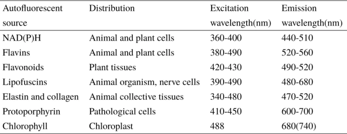
Autofluorescent Distribution Excitation Emission
source wavelength(nm) wavelength(nm)
NAD(P)H Animal and plant cells 360-400 440-510
Flavins Animal and plant cells 380-490 520-560
Flavonoids Plant tissues 420-430 490-520
Lipofuscins Animal organism, nerve cells 390-490 480-680 Elastin and collagen Animal collective tissues 340-480 470-520
Protoporphyrin Pathological cells 410-450 600-700
Chlorophyll Chloroplast 488 680(740)
Table 1.1 – Common biochemical sources of autofluorescence in nature, with their respective emission and excitation maxima. Information summarized from15, 18, 45, 46
Figure 1.1 – Fluorescence excitation (A) and emission (B) spectra of various endogenous tissue fluo-rophores. Spectral shapes are shown for the best relative excitation/emission conditions. The figures are derived from.46
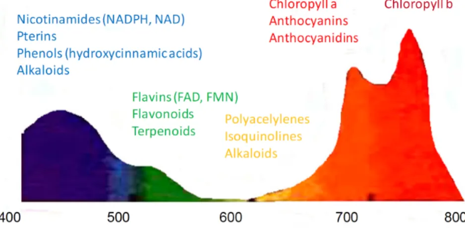
Figure 1.2 – Fluorescence emission spectrum of a typical green leaf under UV-radiation (λexc=355 nm). The fluorescence peaks are found in blue (430-450 nm), green (520-530 nm), red (680 nm) and far red (740 nm) regions. The figure is derived from.15
1.3
State-of-the-art for background reduction in fluorescence imaging
1.3.1 Strategies against the background of ambient light
Spectral analysis
In fluorescence detection, carefully selected optical filters are necessary for discriminating the target fluorescence from the excitation light and the emissions from other ranges of the spectrum. Since the majority of the light sources possess a broad spectrum from UV to IR which covers the emission spectrum of the most commonly used fluorescence probes, spectral filtering has found limited use in elimination of ambient light.
However, the Fraunhofer Line Depth (FLD) method has been exploited to retrieve the red fluorescence signal from the reflected sunlight in sunlight-induced Chlorophyll fluorescence measurements.47 FLD makes use of the dark lines (so-called Fraunhofer lines) of the solar spectrum resulting from the absorption of solar and earth atmospheres, where the fluorescence signal is relatively stronger than the reflected solar intensity and is in consequence detectable. Indeed three main Fraunhofer Lines are found in the red to far-red wavelength range, in which Chlorophyll fluoresces: one hydrogen (H) absorption band is centered at 656.4 nm whereas two dioxygen (O2) absorption bands are centered at 687.0 nm and 760.4 nm. FLD relies on intensity measurements inside and outside of the Fraunhofer lines, and the fluorescence signal is deduced by comparison of the two measurements. In particular, the FLD method measures the incident solar irradiation on the ground level and the radiance from the target plants inside the dark line (λin) and at a wavelength nearby (λout). The method assumes that the reflectance (r) and the fluorescence intensity (F) from the two measured channels are constant, which may give rise to unreliable results. Several methods aiming at improving the accuracy of the FLD measurement have been proposed in the recent decades. Instead of using only one outside band as a reference, one measures two or more bands and adds correction factors to deal with the change of r and F,48, 49 or uses advanced interpolation to get more precise spectral information around the dark lines.50, 51 Further improvement of this method relies on high resolution spectral measurement devices. FLD is a mature method for Chlorophyll fluorescence measurement under daylight. It is suitable not only for ground-based measurement, but also for airborne and even spaceborne fluorescence imaging. However this method is exclusively adapted to Chlorophyll measurement of vegetation under solar light condition, which limits its applications elsewhere.
Dynamic excitation methods
Difference imaging While it is difficult to find a common way to block out the ambient light, a lot of
efforts have been made to enhance the fluorescence intensity itself by playing with the excitation light, so as to reduce the contribution of the ambient light.
The easiest way is to do a subtraction between the images recorded with and without illumination of excitation light. The major disadvantage of this method is due to the fact that the noise induced by the high level ambient light cannot be eliminated by the image subtraction. If the fluorescence intensity is at the same level or even lower than the noise level, the signal would be hard to be detected.
This method has been implemented by using a self-reset complementary metal-oxide-semiconductor image sensor to record the fluorescence image of the Green Fluorescent Protein (GFP) expressed in a
of overexposure by reseting the output value of each pixel when the number of photons received exceeds its threshold. This sensor permits one to collect more fluorescence signal by increasing the exposure time with a reduced noise level of the ambient light. Two images were captured with and without the excitation light under room lighting condition and the difference between them was calculated to retrieve the fluorescence image.
Subtraction has also been applied to detect fluorescence in plants.53 A reference spectrum was first measured under broad-band artificial light. Then a second spectrum was acquired with an additional excitation UV light. The fluorescence spectrum extracted after subtracting the reference was used to analyze the Chlorophyll fluorescence signal and monitor the water stress.
As simple as it is, the subtraction method has limited interest in fluorescence detection under conditions of high level of ambient light, as well as under a temporally varying lighting environment.
Pulsed-light excitation Pulsed excitation light with gated detection is a more commonly used approach for fluorescence imaging under ambient light. The pulsed excitation light is usually generated with a flash lamp or Light Emitting Diode (LED) source with a duration of millisecond down to microsecond, in order to reach an instantaneous intensity more than 10 times the maximum intensity in continuous mode. The camera is synchronized with the flash at a fast shutter speed. Such a system allows not only to enhance the instantaneous fluorescence response, but it also reduces the exposure time to diminish the input of ambient light intensity, which results in an obvious elevation of the fluorescence to background ratio.54, 55 In practical applications, the image captured during the pulsed excitation is corrected with an image previously recorded in the absence of the excitation pulse, to further eliminate the contribution of the ambient light.56, 57 An optimized strategy was recently proposed to avoid the error signals during the subtraction caused by periodically current-driven ambient light in the operating room.58 The pulses were synchronized with the frequency of the background light such that the pulses and the acquisitions occured at the lowest point of the background light intensity. Several devices based on this approach have been developed and applied under various lighting environments,54, 55, 57–60 from room light to sunlight conditions, performing reliable and sensitive fluorescence imaging ability (see Fig.1.3).
Lock-in detection by light modulation Another approach to distinguish a fluorescence signal from the
ambient background relies on lock-in imaging, in which the intensity of the excitation light is modulated at a certain frequency. The fluorescence intensity is consequently modulated with the pace of the excitation light at which any modulation of the ambient light background can be neglected. By applying a time domain Fourier transform, the modulated component of the fluorescence is extracted while the background is filtered.
This method has been successfully applied for fluorescence detection of a bacterial sensor in the soil under daylight condition.61 A more complicated protocol based on modulating both the excitation light and the ICCD sensor was demonstrated in another work for fluorescence imaging of a living animal.62 In this imaging system, the recorded images are phase sensitive. Their intensity depends on the phase delay (η) of the modulation signals between the excitation light and the gain of the ICCD. The fluorescence image containing the modulated component was calculated from three images acquired with different η
Figure 1.3 – Leaf fluorescence using flash versus continuous illumination (CI). Flash illumination was compared against CI from a 100 W Xenon arc lamp, both equipped with the same bandpass filter as part of the chlorophyll filter set (450/50 excitation filter, 740/140 emission filter). The comparison was done on an equal-exposure-time basis, 25 µs exposures or one 900 µs exposure respectively. Therefore, the light dose for imaging the specimen was approximately 180-fold greater under flash illumination. Artificial shaded sunlight from incandescent lamps was set equal to daylight level (10% of full insolation) in the field of view. Ambient (a), and ambient + CI (b) images of the test specimen, a leaf on sand; (c) digital difference image (b) minus (a); summed nonflash (e) and flash images (f); (g) digital difference image (f) minus (e). Graphs (d) and (h) show line profiles of fluorescence across the leaf image at the position indicated by horizontal white lines in panels (c) and (g) respectively. Figure derived from.60
(see Fig. 1.4). Compared to the pulsed excitation approach, the lock-in strategy enables one to gain higher Signal-to-Noise-Ratio (SNR) thanks to a frequency-domain noise filtering. In addition, this strategy is insensitive to irregular fluctuation of the ambient light, which is an advantageous with respect to the other approaches reported above.
1.3.2 Strategies against a background of autofluorescence
Choice of optical filter sets
A typical fluorescence imaging microscope necessitates a fluorescence filter set, which usually consists of three components: an excitation filter, a dichroic beamsplitter, and an emission filter. The fluorescence filter set is used to separate the excitation and the emission optical pathway, as well as to confine the band pass of both channels in order to avoid the interference of excitation light and enhance the fluorescence intensity from the specific fluorescent reporter. As such, the bandpass of the filters should be particularly
Figure 1.4 – iRFP fluorescence images acquired at the phase delay (a) 0◦, (b) 90◦, (c) 180◦ from a representative mouse. (d) The extracted image of AC amplitude. (e) CW Image of DC. (f) Spectra of the fluorescent room lights acquired in the surgical suite showing far red energy. The arrows point to the breast cancer location and the dashed circles represent the background ROIs. Figure derived from.62
picked up to match the excitation and emission band of the fluorophores that one wants to observe. In current fluorescence microscopy, the standard filter sets are TRITC, FITC, and DAPI for red, green, and blue fluorescence respectively. These standard filter sets can eliminate autofluorescence in these wavelength ranges, when it is less intense than the reporter fluorescence. However they cannot filter out the whole autofluorescence background since the latter covers the whole visible region (see Fig. 1.1), which overlaps the emission peaks of all the fluorophores.63
In practice, one can personalize the filter combinations for more specific observations. Considering that autofluorescence arises from a large gamme of unknown natural molecules, which exhibit different absorption bands, an excitation light with a broad spectrum may lead to a stronger autofluorescence signal since more endogenous fluophores tend to be excited. In this case, excitation filters with narrower bandpasses are ideal to limit the autofluorescence to those whose excitation band overlaps that of the reporter fluorophore.64–67
The choice of the emission filter plays a more important role in distinguishing the fluorescence signal. Since the reporter fluorophores exhibit narrow emission spectra with specific peaks, narrow bandpass filters centered around these peaks are often used to augment the contribution of the reporter signals against the non specific broad band autofluorescence. The use of dual bandpass filters has also been reported in fluorescence imaging.65, 67 In a recent work,67an optimized filter set was described and used
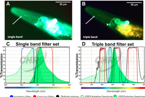
for GFP imaging in Caenorhabditis elegans to overcome the problem of autofluorescence. The proposed filter set used (i) an excitation filter with a very narrow bandwidth of 10 nm centered at the maximum excitation peak of GFP (488 nm) and (ii) more particularly a dual band emission filter with a first pass at 520/20 nm for the GFP emission peak (509 nm) and a second pass at 595/40 nm for the autofluorescence signal. By using a RGB camera, the autofluorescence signal passed through both bands, which appeared yellowish, while the GFP signal was observed mainly through the first pass and remained green (see Fig. 1.5). Compared to broad band filtering, this filter set optimized both the excitation and emission part, firstly to minimize the induced autofluorescence signal from the specimen, secondly to distinguish the color rendering of the GFP signal and autofluorescence signal. Albeit the contrast was enhanced, this method did not truly reduce the autofluorescence background. Moreover it cannot deal with the case when the GFP signal is weaker than the autofluorescence of the same bandpass.
Figure 1.5 – The LSD2022 C. elegans strain expresses an integrated collagen::GFP transgene (ROL-6::GFP), which is visible in the cuticle (white arrow). In addition, the strain LSD2022 expresses GFP driven by the ttx-3 promoter in the AIY interneuron pair (white arrowhead). (A) C. elegans worm (LSD2022) imaged with a commonly used single band filter set (C). (B) The same animal imaged with the triple band filter set (D), where Green is GFP and yellow is autofluorescence. The figure is derived from.67
.
Instead of remaining in the visible region, near infrared fluorescence (NIR) imaging has been another strategy to get rid of the problem of autofluorescence,68, 69 since very few intrinsic fluorophores emit fluorescence beyond 650 nm in the NIR region.70 Further studies have shown that the second NIR region (1200-1800 nm) is even more favorable than the NIR region (650-950 nm), since the autofluorescence contribution at the former region is almost negligible.19, 71 Hence fluorescence imaging in the NIR region has been widely adopted to investigate biological systems in order to obtain an autofluorescence-reduced background.72–76 Although a variety of near infrared dyes such as Indocyanine Green (excitation peak
new NIR emitting fluorophores with higher quantum yield and biocompatibility.
Choice of the growth medium
Fluorescence detection of cells and microbes can also suffer from autofluorescence interference from the growth media the autofluorescence of which can be intense20 and sometimes variable due to cell secretion.77 To generate suitable growth conditions for microbes, growth media are often rich in nutrients, including vitamins such as vitamin A and riboflavin, which are main sources of autofluorescence. The PBS buffer can be used to wash away the fluorescent culture medium right before recording an image. However the medium removal influences the longevity of cells and hampers long-term observation. Various alternatives exhibiting significantly reduced autofluorescence than traditional culture media (E.X. agar gel, LB culture,. . . ) have been reported.45, 78, 79 Although low autofluorescence culture media are not always available for specific uses, the choice of the culture medium should be considered at first if possible, since it is one of the easiest approaches to circumvent the autofluorescence problem.
Chemical treatment
Autofluorescence from cells or tissues can be diminished by specific chemical treatments. Sodium boro-hydride has proven useful to quench autofluorescence induced from aldehyde or formalin fixatives.80–82 Riboflavin can be reduced to a non-fluorescent state by injection of a sodium dithionite solution.83 Copper sulfate can be used to quench lipofuscin-like autofluorescence84and reduce haemosiderin-laden macrophages autofluorescence.85 A series of diazo dyes like trypan blue82, 86, 87and Sudan black B88–91 can be used to mask or absorb visible autofluorescence emission in tissues. They are frequentely adopted in immunofluorescence applications.92, 93 However these dyes are usually applied after immunofluores-cent labeling, which causes also signal reduction of the labels. Such treatments are often combined for better diminishing of the autofluorescence background.82, 94–97
Photobleaching treatment
The autofluorescence of biological samples tends to fade after long time UV irradiation, due to photo-bleaching of the autofluorescent molecules. Photophoto-bleaching refers to photo-induced chemical alteration of the fluorescent molecule such that it is permanently disabled to fluoresce.98 This irreversible destruction of the fluorophore is troublesome in most cases. Nonetheless, it has been an useful tool for diminishing unwanted autofluorescence of animal tissue such as brain, liver and lung.99–102 It has been evidenced that UV irradiation (20 W) should last for at least 24 h to get a significant autofluorescence reduction through the whole sample, and after a treatment of 48 h, most of the autofluorescent background was faded.99 In another work,100 a high power multispectral LED array (240 W) was adopted as the irradiation source, and the process was shortened to 4 h with 80% autofluorescence reduction, which reached 90% after 24 h. Albeit the sample is often photo-treated prior to immunolabeling so as to avoid to affect the label fluorophores, the photo-treatment has also been done after labeling, with cooling during irradiation in order to preserve the quality of the fluorescence marker. It has been additionally shown that fluorescent
proteins like GFP are relatively resistant to photobleaching.45 Due to the chromophore encapsulation, they exhibit a lower bleaching rate than small fluorophores.103, 104 In any case, one should be aware that UV irradiation can easily jeopardize inner components that are critical to the cell activities, which might not be suitable for real time monitoring in situ, not to mention the time consuming pretreatment.
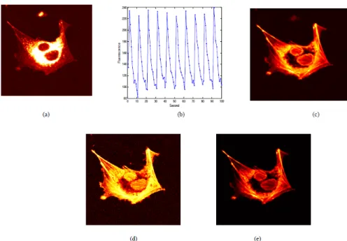
Figure 1.6 – Effect of autofluorescence removal on image quality in the case of FTLD-T tissue with anti-phosphorylated tau immunostaining.(a-c) Low magnification, composite immunofluorescence images of representative fields of view in untreated (a), photobleached for 48 h (b) and chemical quencher treated (c) samples. Colors represent fluorescence in the following channels via excitation by their respective light sources: Alexa 488 (green): λex= 488 nm (argon laser) λem= 493-570 nm; Texas Red (red): λex= 561 nm (DPSS 561 nm laser), λem= 601-635 nm; DAPI (blue): λex= 405 nm (Diode 405 laser), λem= 410-507 nm. Scale bar = 100 µm. (d-r) Higher magnification images of the dotted regions in untreated (d-g), photobleached (i-l) and chemical quencher treated (n-q) samples, with separate fluorescence channels, merged image, and quantified fluorescence signal profiles. Dotted lines in the merged channels (g, l, q) represent the line on which signal profiles (h, m, r) were generated. Scale bar = 50 µm. Autofluorescent particles (af), immunolabeled tau fluorescence (tau) and nucleus signal (nuc) are indicated. The figure is derived from.102
1.3.3 Strategies overcoming interferences of both ambient light and autofluorescence
In the previous section, we introduced several methods for reduction of sample autofluorescence by chemical or photochemical treatments. All of them have significant disadvantages: (i) the choice of the biological media is limited for certain specimens, with a compromise for the cell growth condition;
of the labeling intensity. Furthermore the chemical or photo-toxicity have to be carefully investigated, which limits their applicability to in vivo observations. By contrast, optics-based strategies provide a non-invasive way to investigate biological samples without physical or chemical intrusions. However, intensity detection based on light perturbations have got trouble to eliminate the nuisance of autofluorescence, since both the autofluorescence background and the fluorophore signal are responsive to the excitation light. This section will focus on reviewing several optical imaging techniques exploiting different types of kinetic features of fluorophores,105relying on light as a perturbation parameter and signal processing to retrieve the fluorescence of interest from both ambient light scattering and autofluorescence background.
Fluorescence Lifetime Imaging Microscopy (FLIM)
Fluorescence lifetime imaging microscopy (FLIM) is an imaging technology exploiting the differences of lifetime of the excited state of fluorophores.106, 107 When a fluorophore is excited by a photon, it relaxes towards the ground state and its probability of being excited then obeys an exponential decay as a function of time. Therefore the observed fluorescence intensity exhibits also an exponential decay. In FLIM, it is the lifetime rather than the direct intensity, which is used to discriminate fluorophores. Being an intrinsic property of the fluorophore, lifetime is independent of the local concentration and the brightness of the fluorophore, but it may vary with its molecular environment.108
Three different ways are generally implemented to extract the lifetime information of the fluorescence. First, time-correlated single-photon counting (TCSPC) relies on the detection of individual emitted photons and the associated delay time of their arrival to build an histogram of the number of photons at different time points.109 Exponential fitting of the histogram then provides the lifetime(s). Second, the fluorophores are excited with a pulsed laser, and the detection is triggered after a series of time delays. The decay lifetime is reconstructed after analysis of the recorded intensities.110 While the two former methods rely on pulsed excitation, FLIM can also be implemented with a frequency-domain detection. This approach generates a modulation of the excitation light. As a consequence, the fluorescence intensity is modulated. The fluorescence lifetime can be determined from its modulation depth and phase delay.107, 111 As FLIM allows one to discriminate fluorescent emitters by the difference of their lifetimes, it has been considered to discriminate autofluorescence as well as the time-independent ambient light. Indeed the background autofluorescence exhibits lifetime ranging from ps to several ns.112–115 Hence the targeted fluorescence can be collected with time-gated detection after the autofluorescence dies out. This approach has been implemented to eliminate the chloroplast autofluorescence in plant cells.116 Since the autofluorescence of the chloroplast declines extremely fast(several ps time scale) whereas the lifetime of the common labels like GFP and YFP is to the nanosecond range, the detection started with a delay of 0.3 ns after the pulse excitation, which allowed to completely remove the autofluorescence with only a slight reduction of the label fluorescence. However, autofluorescence has an average lifetime around 4 ns, overlapping the one of most common organic fluorophores. Expanding the detection delay elevates the contrast but at the price of a loss of the fluorescence intensity sought for. For this reason, engineered long-lived fluorescence probes have been designed to ensure complete decline of the autofluorescence while keeping the desired fluorescence at a considerable level. Hence Jin et al. used lanthanide-based
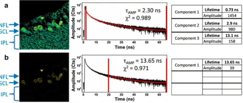
luminescence probes with very long lifetime up to µs and ms.117 Nevertheless these probes have limited photon flux, which lowers the sensitivity. Ryan et al. developed azadioxatriangulenium (ADOTA) dye, the 20 ns lifetime of which is three times longer than usual autofluorophores so as to facilitate detection after the autofluorescence has diminished (see Fig. 1.7).118, 119 More recently, Optical Activated Delayed Fluorescence (OADF) extended the lifetime to tens of µs by exploiting the long live dark state of Ag clusters.120 After a primary pulsed excitation, the Ag cluster is excited to a dark state, which can be depopulated to the excited emissive state by a secondary illumination at longer wavelength with a time delay. Thereby the repumped fluorescence can be activated after fading of the endogenous fluorescence.
Figure 1.7 – Time-gated FLIM applied to tissue labeled with ADOTA. Panel (a) shows the FLIM equivalent of the steady-state image; data collection starts after 2.5 ns and excludes scattered excitation only. In panel (b) data collection is delayed by 10 ns. All of the data shown in this figure were obtained in one collection of data from a single, 80×80 µm (300 pixels × 300 pixels) area of tissue. The figure is derived from.118
By relying on the study of lifetime which is independent of the fluorophore concentration but variable to the molecule context, FLIM is yet not an ideal tool to quantify the local amount of the fluorophore.
Optical Lock-In Detection (OLID)
Several fluorophores exhibit light-driven switch between two states of different brightness, which can be turned on and off reversibly upon illumination of two different wavelengths.121–123 This specific photo-dynamic feature was exploited by G. Marriott et al.124, 125 to isolate the fluorescence signal of the photoswitch from a high level background. Periodic light perturbation drove the fluorophore throughout several cycles of photoswitching and the modulated fluorescence signal of the specific probe was isolated from the constant scattering background as well as the steady autofluorescence background from non-photoswitching sources by what G. Marriott et al. named lock-in detection (OLID). More precisely, the probe was first photoswitched from a dark state to a bright state with a short UV light pulse, and a subsequent excitation light was applied to photoswitch it back to the dark state with a much lower rate. After repeated illuminations over several cycles, the acquired signal from the probe exhibited a sawtooth-like modulation. To amplify the desired signal, a cross-correlation was performed between each pixels of the imaging field and a reference waveform picked from a small region where the fluorophore only was present, so as to analyze the temporal similarity. The cross-correlation coefficient ρ(x, y) at a given pixel
ρ(x, y) =X t
{I(x, y, t) − µI}{R(t) − µR}
σIσR (1.1)
where I(x, y, t) is the detected intensity at pixel (x, y) at time t during the cycle, and R(t) is the reference waveform. µI and µR are the averages, and σI and σR are the standard deviation values of the pixel intensity and the reference waveform respectively.124 With this algorithm, the background (including the ambient light-induced scattering and the autofluorescence which is not supposed to present any photoswitching feature) was not correlated to the reference and thus yielded a cross correlation close to zero. In the contrary, any modulated signal exhibiting a response behavior similar to the reference wave was enhanced, which allowed to selectively display the information of the photoswitchable probe.
OLID was first experimentally demonstrated with reversibly photoswitchable small fluorophore (ni-trospirobenzopyran; nitroBIPS) and genetically encoded fluorescent protein, Dronpa, used to achieve high contrast imaging of living cells and mammalian tissues (Xenopus spinal cord explant and live Zebrafish) free of the artifacts arising from autofluorescence.124 OLID imaging was subsequently also validated with a cyanine probe, which can be photoswitched at high light intensity.126
Eq. (1.1) shows that the modulation intensity is normalized by the STD of the two signals. Thereby the calculated coefficient is not linearly related to the local concentration of the probe. The same team has proposed an optimized method using the “scope” as a weighting factor.127, 128 The scope value is actually the mean peak-valley measured from each pixel during each local cycle:
S(x, y) = N1 N X
i=1
(Lmax(x, y)i−Lmin(x, y)i) (1.2)
where the Lmax(x, y)i(respectively Lmin(x, y)i) is the local maximal (minimal) intensity of the ith cycle, and N is the number of cycles recorded. Meanwhile, the reference point is automatically selected from the pixel possessing the largest scope, without the need of manual process.
The scope values have been used to weight the cross-correlation image127 (see Fig.1.8). While the addition of the scope has taken into account the switching amplitude and further enhanced the contrast as well as the signal-to-noise ratio, the ability of OLID to quantify the local content of the photoswitching probe is still questioned, especially when the background is so overwhelming that the modulation is at the noise level, where the extracted scope is highly unreliable. An erroneously selected reference point leads to alternative correlation analysis (see Fig.1.12), which fails to yield the right OLID image.129 In another work, the scope values were used directly as a weight factor to the raw fluorescence intensity image for the sake of an enhanced contrast.128 Nonetheless, since the final result is coupled with both the scope and the raw intensity (which distorts the real intensity of the fluorescent probe), OLID is not suitable for the quantification of the probe.
Synchronously Amplified Fluorescence Imaging Recovery (SAFIRe)
R. Dickson and his team developed another selective imaging technique called synchronously amplified fluorescence imaging recovery (SAFIRe).130, 131 In their approach, a specific optical modulation strategy is applied so that only the fluorescence of the probe of interest is modulated while the background stays
Figure 1.8 – (a) A single image frame of the living cell (labeled with a non-photoswitchable probe Rhodamine 123 and a photoswitchable protein rs-mcherry-rev) representing peak response to switching; (b) Reference waveform obtained from the fluorescence intensity profile at the selected reference point; (c) Scope image; (d) Results from the correlation image; and (e) Results from the scope-weighted correlation image. The figure is derived from.127
steady. This discrimination exploits a few specific fluorescent molecules, which possess long-lived dark states. When a fluorophore is promoted by light from its ground-state S0 to its excited state S1, it has a certain probability to transit to a dark state T1. When the dark state is long-lived, fluorescence drops even at rather low light intensity. However the population of the dark state can be interestingly reduced upon a secondary illumination with high energy. It regenerates the emissive state S1 faster than the natural decay rate from T1, which thus elevates the fluorescence signal. SAFIRe has implemented this scheme by exploiting several fluorophores in which the depopulation of the dark state occured upon illumination at a wavelength longer than that of the fluorescence emission. While maintaining a constant primary excitation light, optical modulation of the secondary light allowed to dynamically control the population of the emissive state, resulting in a modulated fluorescence intensity. Meanwhile, the collected background was free of the crosstalk from the secondary light with a longer wavelength, therefore remained unmodulated. After performing a time-domain Fourier transformation of the signal from each pixel, the SAFIRe image was reconstructed, where the modulatable probe was amplified whereas the background was removed. Similar to a lock-in amplifier, this scheme allowed to eliminate both autofluorescence and ambient light.
SAFIRe was first validated with Ag nanodots,130and then with organic fluorophores like xanthene131 and Cy5.132 It was later implemented in bioimaging using specific genetically encoded fluorescent proteins, which were able to be photoswitched with the mechanism discussed above. In the first attempt, AcGFP was used to label mitochondria in NIH 3T3 cells while labeling EGFP was introduced elsewhere as a background interference. The image was obtained with a confocal scanning system using an optical
background.133 In another work, SAFIRe was applied in wide field imaging, where a series of engineered BFP mutants modBFP/H148K were found attractive as modulatable labels to enhance the imaging contrast against autofluroescence (see Fig.1.9).134
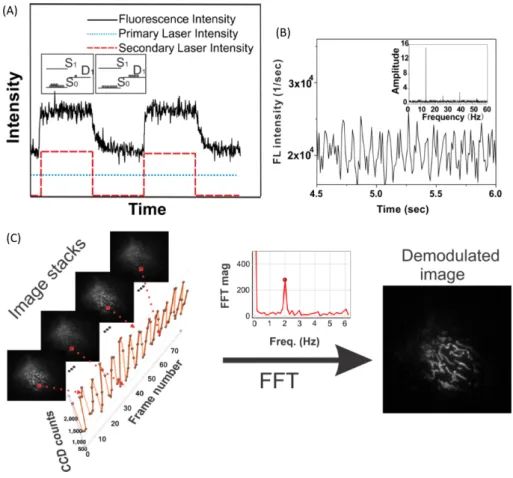
Figure 1.9 – (A) Fluorescence response of an optically modulatable blue fluorescent protein (modBFP/H148K) with constant primary excitation and modulated secondary excitation. The insets show Jablonski diagrams representing dark/bright populations; (B) Time trace of aqueous modBFP/H148K with 372 nm primary excitation and 514 nm secondary excitation modulated at 13 Hz. The inset shows the fast Fourier transform (FFT) of the bulk intensity trajectory, recovering the modulation frequency encoded in the fluorescence signal. (C) Analysis of optically modulated image stacks acquired with SAFIRe by taking the Fourier transform of each pixel’s intensity trajectory. The demodulated image is formed from the FFT amplitude at each pixel. The figure is derived from.135
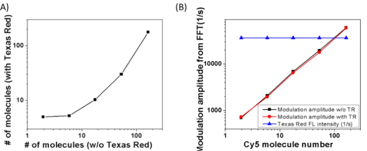
Quantitative measurement of fluorophore concentrations in the presence of an high background was validated by Hsiang et al.,135 using diluted Cy5 solution at varying concentrations with and without a Texas Red fluorescence background. Fig. 1.10A shows the number of Cy5 molecules measured by FCS, respectively in a Texas Red solution and fluorescence-free water. The curve exhibits a non-linearity at low Cy5 numbers, due to the interference of the fluorescence background. In contrast, the FFT amplitude in Figure1.10B reconstructed a quasi-identical linear dependence on the Cy5 concentration in both solutions, devoid of any contribution from the non-modulated background. SAFIRe has also been successfully used in fluorescence correlation spectroscopy (FCS) for background-free quantification of Ag nanocluster.136
Figure 1.10 – (A) Highly nonlinear correlation between the numbers of Cy5 molecules measured by FCS with and without a constant Texas Red background; (B) Plots of the SAFIRe signal (FFT amplitude) vs the number of Cy5 molecules, showing that the modulation amplitude is independent of the presence of the unmodulatable Texas Red background. The figure is derived from.135
A first limitation of SAFIRe originates from constraining the fluorophores to rely on a red-shifted illumination for dark state depopulation to avoid crosstalk. To overcome this limit, Dickson’s research group has proposed a smart approach combining SAFIRe and FRET.137The primary excitation light was applied to the donor, that transfers its energy to the acceptor. Meanwhile a secondary light of longer wavelength than the emission peak of the donor excited the acceptor, giving rise to a competition against the FRET transfer. As a consequence, the intensity of the secondary light was negatively correlated to the fluorescence emission of the donor.
A second SAFIRe limitation originates from constraining the fluorophores to exhibit a long-lived dark state. To avoid seeking dark state fluorophores, Dickson’s research group introduced an all-optical method utilizing simulated emission depletion.138 It exploits the depletion of the fluorescence state by stimulated emission induced by a secondary depletion laser at a longer wavelength than the fluorescence emission, which could be modulated by modulating the depletion laser. The selectivity of this protocol relies on an higher STED efficiency of the targeted fluorophore than the one of the background emitters. Moreover this approach requires high intensities of both primary and secondary lights (mostly attainable in a confocal system), which may generate photobleaching and phototoxicity to the sample and limit its use in real time living cell observations.
A recent work evaluated reversibly photoswitchable fluorescent proteins as labels for SAFIRe imag-ing.129 To avoid the generation of a modulated autofluorescence background which would originate from the high energy secondary light with short wavelength required to depopulate the dark state of RSFPs such as rsFastLime, this work introduced a dual modulation system (DM-SAFIRe), where both the primary and the secondary lights were modulated, but at different frequencies. While the non-photoswitching back-ground independently followed the modulation of the two photoswitching-driving lights, the rsFastLime emission was selectively modulated at both frequencies, which gave rise to a pair of sideband signals (see Fig.1.11) in the Fourier domain completely excluding the background. The superiority of DM-SAFIRe with regards to OLID and SM-SAFIRe in RSFP imaging was established in live NIH-3T3 cells (see
Figure 1.11 – Dual modulation enables background-free rsFastLime detection. rsFastLime interacts with both 405 and 488 nm lasers, while the autofluorescence background is excited independently by each laser. The Fourier transform shows that only rsFastLime presents sideband signals (at 7 and 11 Hz) when the 488 and 405 nm lasers are respectively modulated at 9 and 2 Hz. The figure is derived from.129
Out-of-Phase Imaging after Optical Modulation (OPIOM)
In order to get a more selective kinetic signature of reversibly photoswitchable fluorescent probes, Out-of-Phase Imaging after Optical Modulation (OPIOM) has added the phase lag of the modulated signal to the frequency-dependent modulation depth exploited by SAFIRe for selective imaging. Indeed, OPIOM acts as a band-pass filter for the RSFP signal whereas SAFIRe acts as a low pass filter. As a consequence, OPIOM is more easily prone to direct multiplexed observations of several RSFPs. Moreover OPIOM relies on an exhaustive theoretical frame, which led to extract analytic conditions for its optimal implementation. The OPIOM theoretical framework was first illustrated by Quérard et al.139 It is based on a thorough analysis of the photo-induced switching behavior of a reversibly photoswitchable probe between two states
1 and 2, bright or dark, where the thermodynamically stable state 1 can be photochemically depopulated
to the thermodynamically unstable state 2 with a rate constant
k12(t) = σ12I(t), (1.3)
whereas it is populated back either by photochemical induction or slow thermal recovery at a rate constant
k21(t) = σ21I(t) + k21∆, (1.4)
where σ21I(t) and k∆21are respectively the photochemically-driven and the thermally-driven contributions. Since the exchanging rates between the two states depend on the light intensity I(t), a slight sinusoidal modulation of the light intensity generates a modulation of the population of the two states, but with a phase delay due to the relaxation time of the switch.
i(t) = i0
Figure 1.12 – (A) Signal/background (S/B) comparison of SM- and DM-SAFIRe vs OLID in live NIH-3T3 cells co-expressing untargeted EGFP and mitochondria-targeted rsFastLime: (left to right) raw image, S/B≈1.4; OLID, S/B≈6; demodulated image at 405 nm frequency (SM-SAFIRe), S/B≈5; demodulation at the sideband frequencies (DM-SAFIRe), S/B≈9. (B) S/B comparison in the presence of bright non-rsFastLime background: (left to right) raw live cell image as in (A), S/B≈1; OLID using automatic selection of brightest feature for reference waveform, S/B≈1.6; OLID with manual selection of reference point, S/B≈5; demodulation image upon DM-SAFIRe, S/B≈9. Scale bars = 10 µm. OLID and SM-SAFIRe give similar contrast improvements, and DM-SM-SAFIRe gives a further 2-fold improvement. The figure is derived from.129
where εi1,insin(ωt) and εi1,outcos(ωt) are respectively the in-phase and out-of-phase components of the concentrations at the modulation frequency. Interestingly, further calculation revealed that the i1,in and i1,outvalues are tunable with two modulation parameters: the offset intensity I
0and the angular frequency ω. In particular, the amplitude of the out-of-phase term i1,out exhibits a resonant behavior with a single optimum when the parameters matches:
I0 = k∆ 21 σ12+ σ21 (1.6) ω = 2k∆ 21 (1.7)
where σ12and σ21are the photoswitching action cross-sections of the probe. The optimal conditions are exclusively related to the kinetic features of the probe itself. Since the fluorescence emission is directly related to the population of the bright state, the out-of-phase signal can be extracted from the fluorescence modulation of each pixel simply by temporal Fourier transformation, and used for quantification of the RSFP concentration.
Figure 1.13 – (a) Out-of-phase imaging after optical modulation (OPIOM). A periodically modulated light generates modulation of the signal from reversibly photoswitchable fluorescent probes exchanging between two states (1 and 2), each having a different brightness. The image of a targeted probe is selec-tively and quantitaselec-tively retrieved from the amplitude of the out-of-phase component of the fluorescence emission at angular frequency (ω) upon matching I0 and ω to its dynamic parameters (σ12, σ21, k21∆). (b) Theoretical response of a reversibly photoswitchable fluorophore, 1 2, submitted to light harmonic forcing of small amplitude. The absolute value of the normalized amplitude of the out-of-phase oscil-lations in concentration of 2,
∆2 out nor m
, is plotted versus the light intensity I0 (in ein.s
−1.m−2) and the adimensional relaxation time ωτ120. σ12 = 73 m2.mol−1, σ21 = 84 m2. mol−1, k21∆ = 1.5 × 10⁻²s−1. The figure is derived from.140
(Dronpa-2 and Dronpa-3141) in mammalian cells and zebrafish.140 The images were obtained with a wide field epifluorescence microscope or a single plane illumination microscope by modulating the excitation light from a LED source with a central wavelength of 480 nm. To get the maximal OPIOM response, the modulation parameters [I0, ω] were tuned to match the resonance conditions (Eqs. (1.7)). OPIOM selec-tively visualized the Dronpa-3 labeled structures in the cells, completely rejecting the autofluorescence and EGFP signal which did not exhibit any out-of-phase response (see Fig.1.14). Moreover OPIOM band-pass discrimination enabled to independently image both Dronpa-2 and Dronpa-3 in systems containing both RSFPs.
With a single excitation light at 480 nm, OPIOM relies on repetitive exchange between state 1 and 2 (1 being bright state and 2 being dark state in the case of the Dronpa mutants used), where the population of state 2 is light-driven and recovery of the state 1 occurs with a slow thermal resetting rate of up to several minutes. Under this circumstance, low modulation frequency had to be used to match the resonance. The image acquisition required more than 2 minutes.140 Chen et al. combined SAFIRe131and OPIOM140to achieve a faster imaging rate by introducing a secondary continuous wave light at 405 nm which accelerated the recovery process from 2 to 1.142 The low intensity co-illumination light allowed to drastically increase the light modulation frequency and speeded up the imaging rate to a sub-second time scale.
Figure 1.14 – OPIOM application in mammalian HEK293 cells and in 24 hpf zebrafish embryos. (a,b) Selective imaging of nuclear Dronpa-3 against membrane-localized EGFP. (c,d) Selective imaging of Lifeact-Dronpa-3 against autofluorescence. Fixed (a) or live (b) cells, and zebrafish embryo (c,d) were imaged by epifluorescence (a–c) or single plane illumination microscope (d) (the dashed rectangles indicate the zone illuminated by the thinnest part of the light sheet) upon illuminating with sinusoidal (a–c) or square wave (d) light modulation of large amplitude tuned on the resonance of Dronpa-3. Images labeled Pre-OPIOM and OPIOM correspond to the unfiltered and OPIOM-filtered, respectively, images. Scale bars: 50 mm. The figure is derived from.140
An advanced OPIOM protocol exploiting dual illumination, named Speed OPIOM, was independently introduced by Quérard et al. to increase the frequency of the periodic illumination.143 In Speed OPIOM, both light sources at 480 and 405 nm are modulated in antiphase, leading to a photoswitching between the bright and dark states of the RSFP which is both much faster and of larger amplitude than in OPIOM. Following the theoretical analysis, the fluorescence signal of the RSFP also exhibits a tunable out-of-phase response with a single resonance in the space of the illumination parameters. Interestingly, instead of tailoring the absolute average intensity I0 and the radial frequency ω, one can maximize the Speed OPIOM amplitude only by adjusting the ratios I2/I1and ω/I1to specific values determined by the kinetic photoswitching properties of the RSFP, where I1and I2are the average light intensities at 480 and 405 nm respectively. Moreover, the maximum Speed OPIOM response is twice that in the original one color OPIOM.143 In particular, the resonance conditions show that we can modulate the light sources at higher frequency by increasing both light intensities while keeping constant their ratio, allowing to shorten the imaging time down to the millisecond timescale. Experimental validations have evidenced that Speed OPIOM is a powerful tool for quantitative imaging of reversible photoswitching fluorescent probes, overcoming the autofluorescence background under adverse lighting conditions.
1.4
Objectives of this PhD work
Our group theoretically introduced and experimentally validated the Speed OPIOM protocol for cell obser-vations in fluorescence imaging in works performed before the beginning of this PhD. A simple and cheap homemade epi-fluorescence microscope and a light-sheet fluorescence microscope were respectively de-veloped, with modified illumination systems embedding dual LED or laser sources to achieve two-color