Automatic fixtureless inspection of non-rigid parts based on filtering registration points

(1)

1

Automatic fixtureless inspection of non-rigid parts based on filtering

registration points

Sasan Sattarpanah Karganroudi1_{, Jean-Christophe Cuillière}1(*)_{, Vincent Francois}1_{, Souheil-Antoine Tahan}2 1_{Équipe de Recherche en Intégration Cao-CAlcul (ÉRICCA), Université du Québec à Trois-Rivières, Trois-Rivières, Québec, Canada} 2_{Laboratoire d'ingénierie des produits, procédés et systèmes (LIPPS), École de Technologie Supérieure, Montréal, Québec, Canada}

*Corresponding author: cuillier@uqtr.ca

Abstract

Computer aided inspection (CAI) of non-rigid parts significantly contributes to improving performance of products, reducing assembly time and decreasing production costs. CAI methods use scanners to measure point clouds on parts and compare them with the nominal computer aided design (CAD) model. Due to the compliance of non-rigid parts and for inspection in supplier and client facilities, two sets of sophisticated and expensive dedicated fixtures are usually required to compensate for the deformation of these parts during inspection. CAI methods for fixtureless inspection of non-rigid parts aim at scanning these parts in a free-state for which, one of the main challenges is to distinguish between possible geometric deviation (defects) and flexible deformation associated with free-state. In this work the generalized inspection fixture (GNIF) method is applied to generate a prior set of corresponding sample points between CAD and scanned models. These points are used to deform the CAD model to the scanned model via finite element non-rigid registration. Then defects are identified by comparing the deformed CAD model with the scanned model. The fact that some sample points can be located close to defects, results in an inaccurate estimation of these defects. In this paper a method is introduced to automatically filter out sample points that are close to defects. This method is based on curvature and von Mises stress. Once filtered, remaining sample points are used in a new registration, which allows identifying and quantifying defects more accurately. The proposed method is validated on aerospace parts.

Keywords

Geometric inspection, non-rigid parts, GNIF, fixtureless inspection, principal curvatures, von Mises stress. 1. Introduction

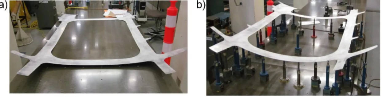
In many industrial sectors, an increasing need for product quality requires respecting smaller and smaller tolerances, which can be obtained by setting up accurate geometric dimensioning and tolerancing (GD&T). Although developments at automating production processes enable manufacturing companies towards mass production with shorter delays, quality control is often time-consuming and usually requires significant human intervention. Geometric dimensioning and tolerancing standards such as ASME Y14.5 and ISO-GPS affirm that inspection of manufactured parts must be carried out in a free-state condition unless otherwise specified. Exemptions to this rule are given in ISO-10579 and ASME Y14.5 (2009) for non-rigid parts. Indeed, in several industrial sectors, such as the aerospace and automotive industries, many manufactured parts are designed and used with a very small thickness with respect to the other dimensions. The problem with these non-rigid (flexible) parts is that they are likely to deform, in a free state, in such a way that the order of magnitude of part deformation may be equal if compared to the part defects itself. For these parts, free-state deformation mainly occurs due to gravity effects (the own weight of the part) or to residual stresses. In [1] the compliance of a part is defined as the ratio between an applied force and the induced deformation in the part. Based on this definition, manufactured parts are classified in three categories as rigid, non-rigid and extremely non-rigid parts. In this classification, a part is considered as a non-rigid part if the deformation induced by a reasonable force (around 40 N) is over 10% of the assigned tolerance. In Figure 1-a, a non-rigid aerospace panel in a free-state deformation due to its compliance is well illustrated.

Consequently, in common inspection methods, as described in [2], dedicated holding fixtures are designed and used to compensate for the flexible deformation of non-rigid parts during inspection. However, these dedicated fixtures are very sophisticated and very expensive to set up in most cases. Thus, in general, geometric inspection of non-rigid manufactured parts is a significant problem since it is expensive and since it takes a large part of production lead-time. For example, some inspection setup for non-rigid parts in aerospace industry requires 60 to 75 hours of operation for setting up one fixture [3]. Meanwhile, a second identical set of fixtures is often required for repeating the inspection at the customer’s facility. In Figure 1-b, the part introduced in Figure 1-a in a free-state is shown as constrained on such a fixture set.

POSTPRINT VERSION. The final version is published here :

Sattarpanah Karganroudi, S., Cuillière, J.-C., Francois, V., & Tahan, S.-A. (2016). Automatic fixtureless inspection of non-rigid parts based on filtering registration points. In International Journal of Advanced Manufacturing Technology (Vol. 87, pp. 687-712).

(2)

2

Figure 1: An aerospace panel, a) in free-state, b) constrained on its inspection fixture [4]

Beholden to the improvements in computer graphics and optic scanners, manual and tactile methods of measurement and inspection have progressively been replaced by Computer Aided Inspection (CAI) methods. CAI methods are noteworthy due to the ability of automating all the inspection process which speeds up and increases the accuracy of inspection by eliminating human intervention and its inseparable error. To evaluate the surface profile of a part, a point cloud measured on part surfaces is compared with the Computer Aided Design (CAD) model. These measurements are performed with two types of geometry acquisition tools: contact and non-contact devices. A review on measuring methods in free-state is presented in [5] and a specific focus is put on using laser scanners in [6]. For non-rigid parts, since coordinate measuring machines (CMM) technology acquires points on the part by means of a probe, which can disturb its geometry due to contact with the probe, using non-contact measurements, such as laser scanners is more appropriate to acquire point cloud of surfaces in a free-state as shown in Figure 2.

Figure 2: Surface data acquisition by a handy scanner.

In CAI, as mentioned above, a point cloud measured on the part surface is compared with the CAD model of this part. The objective is assessing the deviation of these points from the CAD model and comparing it with the tolerances as specified. One of the problems in CAI is that the CAD model is defined in a coordinate system that is not necessarily the same as the coordinate system associated with measured points. Of course, comparison between CAD and scanned models has to be performed in the same coordinate system and in the same state of elastic deformation. As introduced before, measuring non-rigid manufactured parts in a dedicated inspection fixture can solve these problems but, since inspection fixtures such as conformation jigs are costly and time consuming, setting up fixtureless inspections based on CAI methods is foreseen. In these fixtureless inspection methods the non-rigid part is measured in a free-state, and an optimal transformation between the CAD model and the acquired point cloud is computed. For rigid parts, this transformation can be represented by a rigid transformation matrix. For non-rigid parts, finding this transformation is much more difficult since it combines location and orientation along with elastic deformation. This process of finding the best transformation before comparing scan and CAD data is referred to as

registration. Registration methods have been widely studied for rigid parts and several methods have been proposed

[5, 7]. Among these methods, the iterative closest point (ICP) algorithm [8] has been very popular and a source of many adaptations and enhancements for application in various domains (inspection, shape recognition, 3D modeling, robotics, etc. ), which makes it an efficient and robust rigid registration method. As introduced above, non-rigid registration (registration for non-rigid parts) is much more complex since it combines searching for a rigid transformation matrix along with a displacement field. As presented in the next section, a few non-rigid registration methods have been proposed in the literature [3, 9-23]. Basically, these methods try to find the best correspondence between CAD and scan data either by deforming CAD geometry to scan geometry or by deforming scan geometry to CAD geometry.

In general, the main problem is that, the non-rigid registration process is influenced by defects themselves, which are of course not known a priori. Consequently, strategies need to be applied towards reducing, as much as possible,

(3)

3 the influence of defects on the non-rigid registration process and, by the way, towards improving the accuracy and efficiency of CAI for non-rigid parts. This paper is focused on this specific objective.

The paper is organized as follows. Section 2 presents a literature review of fixtureless CAI methods for non-rigid parts. It is followed, in section 3, by a description of the proposed approach towards reducing the influence of defects on the non-rigid registration process in the context of CAI methods for non-rigid parts. This approach is principally based on filtering sample points used in non-rigid registration. Validation of the approach is then presented on two non-rigid aerospace parts in section 4. The paper ends with a conclusion and ideas for future works on this issue in section 5.

2. Literature review

Fixtureless inspection methods of non-rigid parts has been developed relying on numerical approaches to compare the shape of measured parts (represented by scanned point clouds) in a free-state with their nominal CAD model. In order to be able to compensate for flexible deformation of non-rigid parts in a free-state and evaluate the geometrical variation of manufactured parts, either the CAD model is deformed to take on the shape of the scanned model or vice versa. For example, in [9-12] a numerical fixture was proposed to virtually constrain the scanned flexible part into its functional shape. On the contrary, methods proposed in [3, 13-23] are based on numerically deforming the CAD nominal geometry according to the flexible deformation of the measured non-rigid part in a free-state.

The proposed method in [9] begins with acquiring the scanned model of a non-rigid part that is constrained in a reference state. This state does not need to represent the functional state of the part. This scan data in the reference state is used with a first FEA simulation to generate the shape of the part in a completely free state (free from any external forces). From this intermediate result, a virtual functional state of the part is obtained through a second FEA simulation. This virtual functional state is finally compared with the CAD specification for metrology.

In [10, 11], the virtual fixation concept is introduced. It consists in generating a FE model from scanned point cloud in free-state and in identifying, on the scanned part, features such as mounting holes to identify fixation points on the scanned model. Then, this information about the location of nominal fixation points is used to apply displacement boundary conditions to the scanned model, which replicates deforming it to its virtually simulated inspection fixture. However, generating a FE mesh from scanned part requires a time consuming processing on point cloud, which cannot be automated since each measured part needs an individual mesh.

Concerning the automatic FE mesh generating from the CAD model of the part instead of its scanned model, the

virtual reverse deformation method is introduced in [13] wherein the CAD mesh is deformed to conform to the

scanned model of the non-rigid part in a free-state. In this approach, it is done by imposing boundary conditions on the nominal fixation points in the CAD model and displacing these points to the corresponding fixation points in the scanned model, which have been previously identified using feature extraction.

The method proposed in [15] is similar to the virtual reverse deformation method but, in this approach, radial basis functions (RBFs) are used to minimize the FE mesh density. This allows accurately predicting the behavior of the part at a lower computational cost. Meanwhile, in [16, 17] fixtureless inspection is performed by using only partial views of regions that need to be inspected. This is done by applying an interpolation technique, based on RBFs, to estimate an approximate location of the missing fixation points.

In [18] the generalized numerical inspection fixture (GNIF) is presented. This registration method is based on the assumption that, for non-rigid parts, the deformation is isometric, which means that the inter-point shortest path (geodesic distance) between any two points on a part remains unchanged during the isometric deformation. In the GNIF method, CAD and scanned models are considered as geodesic distance metric spaces, and the similarity between them is estimated by finding the associated minimum distortion between the metrics. In this approach, discrete geodesic distances for both CAD and scanned models are calculated, from their meshes, using the fast

marching method [24]. In the GNIF method, generalized multidimensional scaling (GMDS) [25] minimizes the

distortion between the metrics associated with CAD and scanned models. The GNIF method automatically finds corresponding sample points on the faces of CAD and scanned models. The corresponding sample points associated with assembly features are then used for computing the non-rigid registration. Indeed, these corresponding sample points between the two models are used as displacement boundary conditions in a FEA simulation that is applied to deform the CAD model towards the shape of scan data. This process is referred to as finite element non-rigid

registration (FENR). If no information is available about the assembly process, then the sample points on

boundaries of model (assuming boundaries are perfect with no defects on them) or assured sample points with negligible deformations such as rigid attachment are used in FENR. GNIF is improved in [3] as a more general and robust approach referred to as Robust generalized Numerical Inspection Fixture (RNIF). RNIF is based on filtering out sample points causing incoherent geodesic distances. This enhancement enables handling parts with missing range data on surfaces. Meanwhile, the robust GNIF method proposes using distance-preserving nonlinear

dimensionality reduction methods (NLDR) to enhance the inspection process for parts with large deformations. Then

in [26] a review and systematic comparison between NLDR methods are presented in order to evaluate their performance for applications in the metrology of flexible parts.

(4)

4 In [19-22] the iterative displacement inspection (IDI) algorithm is presented along with associated identification methods. By contrast with the methods presented previously, IDI identification concepts are not based on FEA. IDI iteratively deforms the mesh of the CAD model until it matches the shape of scan data. In the IDI algorithm, a specific identification process allows distinguishing flexible deformation from eventual defects on the scanned model surface. Thus, the CAD mesh is smoothly deformed to the scanned shape, except for defects. An improvement of the identification method is proposed in [20] on which the location of points in a measured point cloud is studied statistically to detect defects as outliers with respect to the mean location of neighbor points in the point cloud. This enhancement consists in automatically setting an identification threshold by applying the maximum-normed residual test which is a statistical test to detect outliers in a point cloud.

In [23] another defect identification approach is presented. This approach is based on curvature estimation and Thomson statistical test to identify defects on manufactured parts. This method starts with estimating difference in principal curvatures between the measured point cloud and the nominal CAD model. Then, applying a statistical method (Thomson technique) the suspected outliers of estimated curvature values can be identified and detected as defects. The accuracy of inspections based on IDI method strictly depends on its defect identification algorithm, which can only identify localized defects. On the other words, IDI method cannot evaluate defects distributed in a global manner over a non-rigid part. Meanwhile, the presented identification approach in [23] is not able to identify defects on complex geometry of non-rigid parts by applying solely a threshold for estimated curvature difference. On the other hand, in the above mentioned non-rigid registration methods using FEA for registration, the foreknown assembly information of non-rigid parts are required to specify the location of imposed boundary conditions in FENR.

In the approach presented along the following sections, the location and parameters of boundary conditions used in the non-rigid registration is automatic. Indeed, an initial set of corresponding points between CAD and scanned geometry is automatically filtered to improve FENR, which brings about a better accuracy in the detection of defects on non-rigid parts.

3. Methodology and implementation

3.1. Description of the proposed methodology

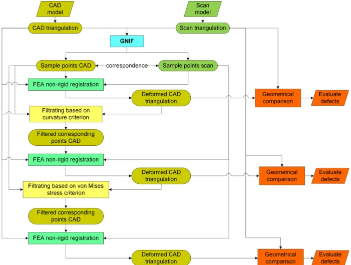
In this paper, the generalized numerical inspection fixture (GNIF) [18] method is first applied as non-rigid registration method to find an initial set of corresponding points between nominal CAD and scan data in a free-state. Indeed, based on the isometric deformation assumption, GNIF generates two lists (one the CAD model and one on the scanned model) of estimated corresponding sample points. Then, these two lists of corresponding sample points are used to deform the CAD model to the scan data via FENR. Since these corresponding sample points are evenly distributed over both models, some of these points can be located close to defects. This results in an inaccurate estimation of the size of these defects. We have shown in a previous preliminary work [27] that filtering sample points that are close to defects in the FENR reduces this inaccuracy. The problem is that these defects are not known a priori. The approach proposed features two stages in filtering these sample points: curvature comparisons and von Mises stress calculations.

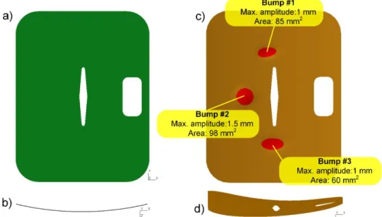
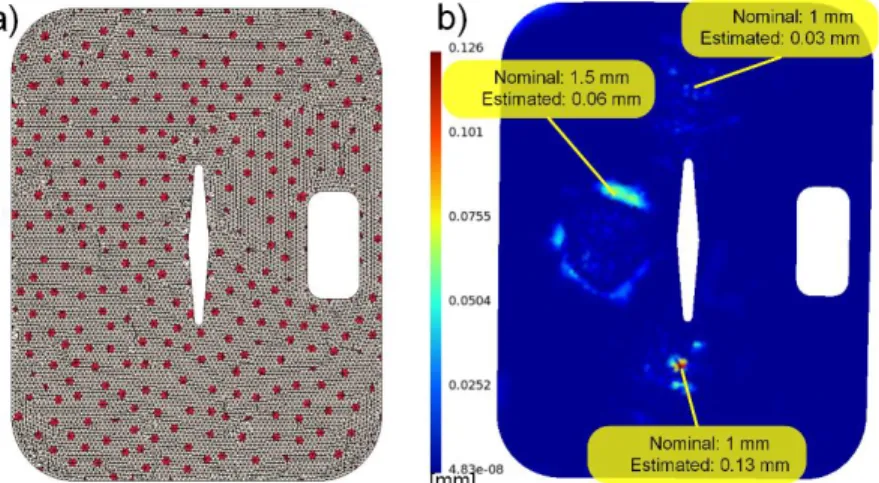
The approach proposed in this paper is described using a typical non-rigid aluminum panel used in the aerospace industry (dimensions are 1100 mm by 860 mm with 1 mm thickness). The CAD model is shown in Figure 3-a, and the associated simulated scanned model for inspection in a free-state in Figure 3-c. This scan data includes three bump defects. The actual (or nominal) size of these defects is known a priori so that the size of defects as identified can be compared with the actual size. The maximum amplitude of a given defect is defined as the distance between the deformed CAD (after non-rigid registration) and scan data at the tip (or valley) of this defect. The area of a

given defect is defined as the area that exceeds the tolerance value, as specified on the drawing. For all validation

cases presented, we considered 0.4 mm as a representative specified tolerance value. Top views of models as shown in Figure 3-b and d, clearly show free-state deformation of scan data.

A pre-registration, based on the ICP algorithm [8], is followed by generating GNIF sample points on both models as shown in Figure 4. These corresponding sample points are then used to impose displacement boundary conditions to deform the CAD model to the scanned model through finite element non-rigid registration (FENR).

Since GNIF CAD sample points are not exactly located on nodes of the CAD triangulation, local modifications are performed on this triangulation before applying FENR. As shown in Figure 5, this is performed using a classical Delaunay point insertion method [28].

(5)

5

Figure 3: A non-rigid aluminum panel a) front view of the CAD model b) top view of the CAD model c) front view of the scanned part in a free-state d) top view of the scanned part in a free-state.

Figure 4: GNIF corresponding sample points (in black) are located in the center of colored zones on CAD and scanned models.

Figure 5: a) The purple point presents a GNIF sample point to be inserted b) the sample point is inserted into the mesh by incremental Delaunay triangulation c) Testing the empty sphere criterion d) swap diagonal operator.

(6)

6 For the sample part introduced in Figure 3, red spots in Figure 6-a represent GNIF sample points after insertion into the CAD mesh. As introduced above, FENR is based on imposing displacement boundary conditions on these sample points to deform the CAD mesh to the shape of scan data. The displacement distribution associated with FENR is shown in Figure 6-b. As shown in Figure 6-a, some of the corresponding sample points on the CAD mesh are located close to defects and/or on defects. These sample points tend to bring the deformed CAD model to the shape of defects in the scanned model, which is obviously a source of error in assessing size and location of these defects. This is well illustrated in Figure 6-c, where the distribution of distance between deformed CAD and scan data is illustrated, and also in Figure 6-d, where the estimation of defects’ area is depicted. Indeed, the size of the 3 defects is under-estimated, due to the fact that some of the sample points used in FENR are close to these defects.

Figure 6: a) GNIF sample points on the CAD model represented as red spots b) displacement distribution [mm] after FENR based on using all GNIF sample points c) comparison between estimated and nominal size of defects

[mm] when using all GNIF sample points d) estimating the area of defects [mm2_].

This result shows that, to avoid deforming the CAD model around defects, the sample points that are located close to these defects should be filtered out. The problem is that these defects are not known a priori. Therefore, as shown in Figure 7, these sample points are filtered after applying a first FENR through the following two steps:

 GNIF sample points filtering based on a local curvature criterion  GNIF sample points filtering based on a von Mises stress criterion

The first filtering step is based on locally comparing principal curvatures of the CAD model before deformation with principle curvatures of the CAD model after FENR (after deformation). This is done at the location of all sample points and it allows a first rough assessment of defects. Indeed, the deformed CAD model obtained using all sample points is almost similar to the shape of scanned model including the defects. Since the flexible deformation of a non-rigid part has a smoother curvature comparing to a defect such as a bump, studying the difference of each principal curvatures between the CAD before and after deformation allows roughly assessing defects. Discrete principal curvatures 𝐾1(𝑝) and 𝐾2(𝑝) are calculated and compared between the two triangulations (CAD and

deformed CAD) using:

𝐾1(𝑝) = 𝐾𝐻(𝑝) + √𝐾𝐻2(𝑝) − 𝐾𝐺(𝑝) (1)

(7)

7 Where KH is the mean curvature and KG is the Gaussian curvature, which are calculated as discrete curvatures

using the Gauss-Bonnet scheme [29].

Figure 7: Schematic diagram of the proposed sample point filtration method.

Note that, since the criterion is based on the difference between curvature distributions and not on the curvature distribution itself, high curvature zones do not cause problems in the process. In section 4.3, the part used (referred to as part B) for validation results features such high curvature zones and results obtained support this statement. Distributions of the difference in discrete principal curvatures between CAD deformed CAD triangulations, are shown in Figure 8-a and Figure 8-b. It clearly shows that areas exceeding a threshold values on these differences represent a rough estimate of defects. The maximum and minimum threshold values of the difference in principal curvatures used are -0.05 and +0.05 mm-1_{. Note that the color scale used in Figure 8-a and Figure 8-b is limited to} these maximum and minimum threshold values. This allows identifying defect zones (defect tip and contour) in blue and red for maximum curvature (K1) in Figure 8-a, and minimum curvature (K2) in Figure 8-b. Threshold values

used are determined based on the mean value of curvature differences, which enables detecting defects as outliers. Based on these threshold, sample points can be filtered inside a radius (3 times the average mesh size ≈ 3 mm here) around sample points that have been identified as close to the defects, as shown in Figure 8-c. In Figure 8-c and other similar figures along the paper, filtered sample points are represented as blue spots while red spots represent sample points that remain after filtering and that will be used in the next step. It appears in Figure 8-c that a few sample points that are not located around defects are also filtered based on this curvature criterion. This is due to local effects introduced by bad mesh quality and noise in the calculation of discrete principal curvatures. However, since a large number of sample points is used (400 points here), FENR is not significantly affected by these over-filtered sample points. Then, a second FENR is applied, using sample points remaining, which leads to a new distribution of distances between deformed CAD and scan data (see Figure 8-d). If compared to the results shown in Figure 6-c and d, results presented in Figure 8-d and e clearly show that the maximum amplitude and area of defects is better estimated from this new registration.

(8)

8

Figure 8: a) distribution of the difference in maximum curvature (K1) [mm-1] b) distribution of the difference in minimum curvature (K2) [mm-1] c) sample points filtered using the curvature criterion (represented as blue spots) d)

comparison between estimated and nominal size of defects [mm] when using sample points after filtering based on the curvature criterion e) estimating the area of defects [mm2_].

As introduced above, a second filter is applied on the remaining sample points. This second filtering step is based on analyzing von Mises stress results (see Figure 9-a) associated with the second FENR. Two conclusions can be made when thoroughly analyzing this von Mises stress distribution:

 von Mises stress is quite high everywhere (the minimum value equals 23.7 MPa), which may seem surprising: this phenomenon is due to the inherent error caused by calculating geodesic distances with the fast marching algorithm (FMA) [24] . Indeed, it is common knowledge that fast marching introduces a bias in the calculation of geodesic distances. We quantified this bias using a shape with similar dimensions for which exact geodesic distances were known and we found that this bias can reach around 1 mm for some sample points. A 1 mm in-plane distance error causes a very high in-plane strain when applying FENR at this location and consequently a very high in-plane stress. This amplitude in geodesic distance error explains the amplitude background von Mises stress noise in Figure 9-a.

 Despite this background von Mises stress noise, remaining sample points that are close to defects feature even higher von Mises stress. This allows filtering a second set of sample points based on this von Mises stress distribution (the first set being filtered based on the curvature criterion).

This second filtering step is based on applying a threshold on the von Mises stress distribution as illustrated in Figure 9-a (the threshold is 1000 MPa in this case). This von Mises stress threshold value is also defined based on the mean value of von Mises stress over the part. Based on this second criterion, new sample points are filtered inside a radius (again 3 times the average mesh size) around sample points that have been identified as close to defects. Blue spots in Figure 9-b illustrate sample points that have been filtered once applied these two consecutive filters. Figure 9-b can be compared with Figure 8-c to evaluate how many new sample points have been filtered and where. Finally, a third FENR is applied, using sample points remaining after applying the two filters, which leads to a third distribution of distances between deformed CAD and scan data along with defects estimation (see Figure 9-c and d). If compared to results shown in Figure 6-c and d as well as Figure 8-d and e, results presented in Figure 9-c and d shows that the size of defects is even better estimated after this last registration.

(9)

9

Figure 9: a) distribution of von Mises stress [Pa] after FENR when using GNIF sample points after filtering based on the curvature criterion b) sample points filtered using both curvature and von Mises stress criteria (represented as blue spots) c) comparison between estimated and nominal size of defects [mm] when using GNIF sample points after filtering based on both curvature and von Mises stress criteria d) estimating the area of defects

[mm2_].

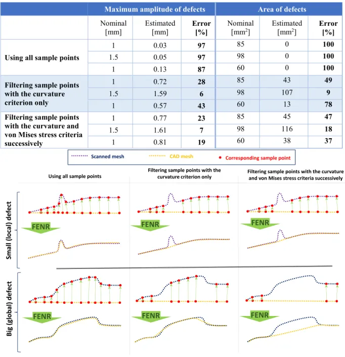
The estimated size of defects and the associated error with respect to the nominal size of defects are summarized in Table 1 for this part. A comparison is presented between errors on the maximum amplitude and area of defects before and after applying the two filters. The average error on the maximum amplitude of defects for the three bumps is 94% before filtering, 26% after applying the first filter and 16% after applying both filters while the average error on area estimation is 100%, 46% and 34% respectively. Thus, the outcome of filtering is a global improvement in the results about estimating the size of defects. Although the error for bump #2 (as identified in Figure 3-c) after filtering based on both criteria is slightly higher than the error based on applying the curvature criterion only, the average error for the three defects is globally decreased by applying both criteria.

As illustrated in Figure 10 results obtained on different types of defects show that in some cases, the second filter does not eliminate many sample points, which makes that estimated errors before and after applying this second filter may not be very different. It also appears that, in some cases, this second filter slightly degrades the estimation. This degradation is related to the fact that some sample points may be filtered, based on von Mises stress, due to GNIF local inaccuracies and not due to the presence of defects. However, this second filter globally improves the estimation since, for bigger defects (see the second case in Figure 10) the flat shape on top of this type of defects makes that there is no difference in principal curvatures and that some sample points are not filtered based on the curvature criterion. As shown in the Figure, these remaining sample points are filtered based on von Mises stress criterion since bringing these sample points to the shape of defect through FENR induces a local stress increase. Thus, applying these two filters successively represents the best compromise for successfully handling different types of defects.

(10)

10

Table 1: Estimated size of defects and errors based on curvature and von Mises criteria for Part A with local defects and bending deformation.

Maximum amplitude of defects Area of defects

Nominal

[mm] Estimated [mm] Error [%] Nominal [mm2_] Estimated _[mm2_] Error _[%]

Using all sample points

1 0.03 97 85 0 100

1.5 0.05 97 98 0 100

1 0.13 87 60 0 100

Filtering sample points with the curvature criterion only

1 0.72 28 85 43 49

1.5 1.59 6 98 107 9

1 0.57 43 60 13 78

Filtering sample points with the curvature and von Mises stress criteria successively 1 0.77 23 85 45 47 1.5 1.61 7 98 116 18 1 0.81 19 60 38 37

FENR

Smal l ( lo cal ) d ef ec t Bi g ( glo b al ) d ef ec t

Filtering sample points with the curvature criterion only Using all sample points

FENR

Filtering sample points with the curvature and von Mises stress criteria successively

Scanned mesh CAD mesh _{Corresponding sample point}

Figure 10: Interest of using the two filters successively.

3.2. Implementation

The implementation of this methodology uses several tools. GNIF calculations for generating sets of corresponding sample points are carried out using a MATLABTM_{code. This code takes approximately 8 minutes for} generating 400 corresponding sample points on a computer with Intel(R)_CoreTM_{i7 at 3.60 GHz with 32 GB RAM.} Mesh generation, mesh transformations, discrete curvature calculations, FENR and distance calculations between deformed CAD and scan models is done using our research platform [30]. This platform is based on C++ code, on Open CASCADETM_{libraries and on Code_Aster}TM_{as FEA solver. We also use Gmsh}TM_{[31] for visualizing 3D} models and distributions (discrete curvature, stress, distance). In general, filtering sample points with the two criteria approximately takes 2 minutes (for a CAD mesh with 10 000 nodes) on a computer with specifications as mentioned above. It should finally be underlined that, since this methodology is based on fast marching, FEA and discrete curvature calculations, final results are quite sensitive to mesh size and mesh quality, both for CAD and scan data.

(11)

11 3.3. Validation on a case with no defects

In this section, our methodology is applied to a case that does not feature any defect. Thus, the only difference between CAD and scan models is due to free-state deformation. This validation aims at verifying that the proposed method has no bias and that no defects are detected. The same model as presented in section 3.1 is used here. GNIF sample points are shown in Figure 11-a and the result of the first FENR (without filtering applied) in Figure 11-b. The distribution of difference in discrete principal curvatures is in Figure 12-a and b. Sample points that are filtered based on curvature are shown by blue spots in Figure 12-c and the resulting second FENR in Figure 12-d.

Figure 11: a) GNIF sample points on the CAD model represented as red spots b) comparison between deformed CAD and scanned models when using all GNIF sample points [mm].

Figure 12: a) distribution of the difference in maximum curvature (K1) [mm-1] b) distribution of the difference in minimum curvature (K2) [mm-1] c) sample points filtered using the curvature criterion (represented as blue spots) d)

comparison between deformed CAD and scanned models when using GNIF sample points after filtering based on the curvature criterion [mm].

(12)

12 In Figure 13-a, the distribution of von Mises stress after this second FENR is depicted. As introduced in section 3.1, although there are no defects in this case, the mean von Mises stress is quite high (around 500 MPa). This quantifies the in-plane background von Mises stress noise introduced in section 3.1, which is due to in-plane distance errors in the calculation of geodesic distances.

Sample points that are filtered based on both curvature and von Mises stress are shown in Figure 13-b and the resulting third FENR in Figure 13-c. A closer look at Figure 11-b, Figure 12-d and Figure 13-c shows that, when no defects are applied, FENR achieves very good results in general, except in the upper left zone where the maximum distance is around 0.2 mm. However, this distance remains under the tolerance (0.4 mm) which makes that, at the end, no defects are identified. It also shows that, as expected here because no defects are applied, the more sample points are filtered, the worse FENR gets. Thus, if the process tends to filter too many sample points, it may result in identifying defects that are not actual defects. On the contrary, if the process tends to filter less sample points than required around defect zones, it may result in missing actual defects or underestimating the size of defects.

Figure 13: a) distribution of von Mises stress [Pa] after FENR when using GNIF sample points after filtering based on the curvature criterion b) sample points filtered using curvature and von Mises stress criteria (represented

as blue spots) c) comparison between deformed CAD and scanned models when using GNIF sample points after filtering based on both curvature and von Mises stress criteria [mm].

4. Results

4.1. Introduction : validation cases

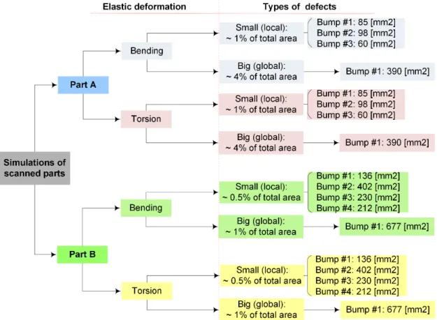
In this section, performance of the proposed approach is validated on two aluminum parts (referred to as part A and part B) with different types and sizes of defects and different types of free-state deformation. Part A is the part used in the previous section and part B is is also typical of non-rigid parts used in the aerospace industry. Several validation cases have been considered for these parts, which are summarized in Figure 14. Two types of free-state deformation are applied (referred to as bending and torsion) and both small (local) and big (global) defects are simulated for each part, as shown in Figure 14.

Thus, four case studies are performed on each part and, for each case, comparisons are made between estimated and nominal size of defects:

 using all sample points (without filtering)

 after filtering sample points based on the discrete curvature criterion only  after filtering sample points with curvature and von Mises criteria successively

In all cases, initial GNIF sample points in the CAD model are illustrated as red spots (●) while filtered sample points, based on either curvature or von Mises stress criteria, are illustrated as blue spots (●). Meanwhile, color scales for the distribution of curvature differences are based on the maximum and minimum threshold values, while color scales for von Mises stress distributions is based on the von Mises stress threshold and on the minimum von Mises stress value.

(13)

13

Figure 14: Synthesis of validation cases.

4.2. Validation cases for part A

Part A is presented in Figure 3-a and Figure 3-b. In its nominal state (without deformation and defects), it features a single and almost constant 0.005 mm-1 _{curvature over the whole panel. The flexible deformation of scanned model} in free-state for this part is simulated by bending and torsion as introduced in Figure 14 and as shown in Figure 15. Note that top view of part A under bending deformation is also shown in Figure 3-d. As introduced in the previous section, thresholds used for the curvature criterion are -0.05 and +0.05 mm-1_{and the threshold used for the von} Mises stress criterion is 1000 MPa.

Figure 15: Side view of the CAD model for part A (in green) compared with the scanned model in a free-state (in brown) with a) bending deformation b) torsion deformation.

The first validation case associated with part A has been presented in section 3. Results show that, in this case, the average inspection error (for amplitude and area of defects) significantly decreases when using the two filters.

In the second validation case associated with part A, the scanned model in a free-state is simulated by applying torsion and three local bumps are also imposed as defects. Initial GNIF sample points and associated estimation of defects are shown in Figure 16.

(14)

14

Figure 16: Part A with local defects and torsion a) GNIF sample points on the CAD model represented as red spots b) comparison between estimated and nominal size of defects [mm] based on using all GNIF sample points.

Distributions of the difference in discrete principal curvatures between the CAD model and the deformed CAD model (using all GNIF sample points) are shown in Figure 17-a and b. As explained in the previous section and as shown in Figure 17-c, after applying the curvature criterion, some sample points located around defects are removed and Figure 17-d illustrates the effect on the results after FENR.

Figure 17: Part A with local defects and torsion a) distribution of the difference in maximum curvature (K1) [mm -1_{] b) distribution of the difference in minimum curvature (K}₂_{) [mm}-1_{] c) sample points filtered using the curvature} criterion (represented as blue spots) d) comparison between estimated and nominal size of defects [mm] when using

GNIF sample points after filtering besed on the curvature criterion.

In Figure 18-a the von Mises stress distribution associated with this FENR is illustrated and, as shown in Figure b, after applying the von Mises stress criterion, some more sample points are removed around defects. Figure

(15)

18-15 c, shows the result obtained after the last FENR. A summary of quantitative results, for this second validation case on part A, is provided in Table 2. These results show that the estimation of the maximum amplitude of defects is slightly degraded for one defect (bump#3 as illustrated in Figure 3-c) after filtering sample points based on both curvature and von Mises criteria. However, the average estimation error for maximum amplitude, using all sample points, filtering sample points with the curvature criterion only and filtering sample points with the curvature and von Mises stress criteria successively, for the three bumps, is 93%, 13% and 10% respectively; while the average area estimation error, for the three bumps, is 100%, 27% and 20% respectively. Here again, the average estimation error for the three defects is decreased by applying both criteria if compared to applying the curvature criterion only.

Figure 18: Part A with local defects and torsion a) distribution of von Mises stress [Pa] after FENR based on GNIF sample points after filtering using the curvature criterion b) sample points filtered using curvature and von Mises stress criteria (represented as blue spots) c) comparison between estimated and nominal size of defects [mm]

when using GNIF sample points after filtering based on both curvature and von Mises stress criteria. Table 2: Estimated size of defects and errors based on curvature and von Mises criteria for part A with small

defects and torsion deformation.

Nominal

1 0.03 97 85 0 100

1.5 0.06 96 98 0 100

1 0.13 87 60 0 100

1 0.73 27 85 38 55

1.5 1.55 3 98 101 3

1 0.91 9 60 46 23

Filtering sample points with the curvature and von Mises stress criteria successively

1 0.81 19 85 54 36

1.5 1.53 2 98 99 1

1 0.9 10 60 47 22

In the following paragraph, as presented in Figure 14, two other validation cases are applied on part A. These cases aim at evaluating ability of our method in identifying big (global) defects. In the third validation case for part A, the scanned model in a free-state is simulated by applying bending. Initial GNIF sample points and the associated estimation of the size of defects are shown in Figure 19. Distributions of the difference in discrete principal curvatures between the CAD model and the deformed CAD model (using all GNIF sample points) are shown in Figure 20-a and Figure 20-b. Figure 20-c shows sample points that are filtered after applying the curvature criterion and Figure 20-d illustrates the effect on the results after FENR. In Figure 21-a the von Mises stress distribution associated with this FENR is illustrated, and as shown in Figure 21-b after applying the von Mises stress criterion, some more sample points are removed around defects. Figure 21-c, shows the result obtained after the last FENR. A summary of quantitative results, for this third validation case on part A, is provided in Table 3. In this validation test, the error in estimating the size of this bigger defect is decreased after filtering sample points based on both curvature and von Mises criteria if compared to applying the curvature criterion only.

(16)

16

Figure 19: Part A with a global defect and bending a) GNIF sample points on the CAD model represented as red spots b) comparison between estimated and nominal size of defects [mm] when using all GNIF sample points.

Figure 20: Part A with a global defect and bending a) distribution of the difference in maximum curvature (K1) [mm-1_{] b) distribution of the difference in minimum curvature (K}₂_{) [mm}-1_{] c) sample points filtered using the} curvature criterion (represented as blue spots) d) comparison between estimated and nominal size of defects [mm]

(17)

17

Figure 21: Part A with a global defect and bending a) distribution of von Mises stress [Pa] after FENR when using GNIF sample points after filtering based on the curvature criterion b) sample points filtered using curvature

and von Mises stress criteria (represented as blue spots) c) comparison between estimated and nominal size of defects [mm] when using GNIF sample points after filtering based on both curvature and von Mises stress criteria.

Table 3: Estimated size of defects and errors based on curvature and von Mises criteria for Part A with big defects and bending deformation.

Nominal

Using all sample points 1.5 0.07 95 390 0 100

Filtering sample points with the curvature

criterion only 1.5 1.73 15 390 283 27

1.5 1.71 14 390 352 10

In the last validation case associated with part A, the scanned model in a free-state is simulated by applying torsion and a big defect is applied. Initial GNIF sample points and the associated estimation of the size of defects are shown in Figure 22. Distributions of the difference in discrete principal curvatures between the CAD model and the deformed CAD model (using all GNIF sample points) are shown in Figure 23-a and Figure 23-b. Figure 23-c shows sample points that are filtered after applying the curvature criterion and Figure 23-d illustrates the effect on the results after FENR. In Figure 24-a the von Mises stress distribution associated with this FENR is illustrated and, as shown in Figure 24-b after applying the von Mises stress criterion, some more sample points are removed around defects. Figure 24-c, shows the result obtained after the last FENR. A summary of quantitative results, for this last validation case on part A, is provided in Table 4. In this validation test, the error in estimating the maximum amplitude of this defect is degraded after filtering sample points based on both curvature and von Mises criteria if compared to applying the curvature criterion only. Although in this case, it appears that filtering based on the von Mises criterion does not improve accuracy in the maximum amplitude estimation of defects, but the area of defect is estimated more accurately.

(18)

18

Figure 22: Part A with a global defect and torsion a) GNIF sample points on the CAD model represented as red spots b) comparison between estimated and nominal size of defects [mm] when using all GNIF sample points.

Figure 23: Part A with a global defect and torsion a) distribution of the difference in maximum curvature (K1) [mm-1_{] b) distribution of the difference in minimum curvature (K}₂_{) [mm}-1_{] c) sample points filtered using the} curvature criterion (represented as blue spots) d) comparison between estimated and nominal size of defects [mm]

(19)

19

Figure 24: Part A with a global defect and torsion a) distribution of von Mises stress [Pa] after FENR based on GNIF sample points after filtering using the curvature criterion b) sample points filtered using curvature and von Mises stress criteria (represented as blue spots) c) comparison between estimated and nominal size of defects [mm]

when using GNIF sample points after filtering based on both curvature and von Mises stress criteria. Table 4: Estimated size of defects and errors based on curvature and von Mises criteria for Part A with big

defects and torsion deformation

Nominal

Using all sample points 1.5 0.04 97 390 0 100

criterion only 1.5 1.76 17 390 300 23

1.5 1.85 23 390 398 2

4.3. Validation cases for part B

Next validation cases are intended to illustrate applying our method on a different type of non-rigid part (see Figure 25). It a long formed aluminum non-rigid part used in the aerospace industry with more complex features, smaller details and higher curvatures (channel section is 40 mm by 20 mm with 1 mm thickness and channel length is 1150 mm). As introduced in section 4.1, two types of defects are applied on this part as well as two types of free-state deformation. Defects are assessed on part B using the same methodology as for part A except for threshold associated with curvature and von Mises stress criteria which are determined based on new mean values for this part. Negative and positive local curvature difference threshold values for part B are -0.01 and +0.01 mm-1_{and the von} Mises stress threshold is 400 MPa.

(20)

20 The initial corresponding sample points between CAD and scanned models are shown in Figure 26.

Figure 26: GNIF corresponding sample points (in black) on the CAD and scanned models of part B.

The free-state deformation of scanned model for part B is also simulated with bending and torsion as presented in Figure 27 and two types of defects are applied as for part A: small (local) and big (global) defects.

Figure 27: Side view of CAD model for part B (in green) compared with the scanned model (in brown) a) with bending deformation b) with torsion deformation.

In the first validation case for part B, free-state deformation is bending and four local bumps are imposed. Initial GNIF sample points and the associated estimation of the size of defects are presented in Figure 28-a and b. Distributions of the difference in discrete principal curvatures (using all GNIF sample points) are shown in Figure 28-c and d. The von Mises stress distribution associated with the second FENR is presented in Figure 28-e. Sample points removed after applying the two filters are illustrated in Figure 28-f and Figure 28-g, shows results obtained after the last FENR.

(21)

21

Figure 28: Part B with local defects and bending a) and f) initial and filtered sample points c) and d) distribution of the difference in principle curvatures [mm-1_{] e) distribution of von Mises stress [Pa] after the second FENR. b)} and g) comparison between estimated and nominal size of defects [mm] based on initial and filtered sample points.

A summary of quantitative results, for this first validation case on part B, is provided in Table 5. In this case, the error in estimating the maximum amplitude of these defects is slightly degraded for two bumps (among four) after filtering sample points based on both curvature and von Mises criteria if compared to applying the curvature

(22)

22 criterion only. However, the average estimation error for maximum amplitude, using all sample points, filtering sample points with the curvature criterion only and filtering sample points with the curvature and von Mises stress criteria successively, for the four bumps, is 60%, 8% and 8% respectively; while the average area estimation error, for the four bumps, is 83%, 9% and 7% respectively. Therefore, the average error is globally decreased by applying both criteria.

Table 5: Estimated size of defects and errors based on curvature and von Mises criteria for Part B with small defects and bending deformation.

Nominal

1 0.36 64 136 0 100

2 0.62 69 402 50 88

2 1.01 50 230 70 70

1.5 0.62 59 212 56 74

1 0.89 11 136 118 13

2 1.88 6 402 378 6

2 1.92 4 230 239 4

1.5 1.35 10 212 184 13

1 0.88 12 136 118 13

2 1.88 6 402 378 6

2 1.89 6 230 228 1

1.5 1.39 7 212 199 6

In the second validation case associated with part B, the scanned model in a free-state is simulated by applying torsion, while four local bumps are imposed as defects. Initial GNIF sample points and the associated estimation of the size of defects are shown in Figure 29-a and b. Distributions of the difference in discrete principal curvatures between CAD and deformed CAD models (using all GNIF sample points) are shown in Figure 29-c and d. The von Mises stress distribution associated with the second FENR is presented in Figure 29-e. Sample points removed after applying the two filters are illustrated in Figure 29-f and Figure 29-g, shows results obtained after the last FENR. A summary of quantitative results, for this second validation case on part A, is provided in Table 6. In this case, the error in estimating the maximum amplitude of these defects is slightly degraded for one of the four bumps after filtering sample points based on both curvature and von Mises criteria if compared to applying the curvature criterion only.

However, the average estimation error for maximum amplitude, using all sample points, filtering sample points with the curvature criterion only and filtering sample points with the curvature and von Mises stress criteria successively, for the four bumps, is 57%, 17% and 15% respectively; while the average area estimation error, for the four bumps, is 78%, 18% and 16% respectively. Thus, like in previous cases, the average error is globally decreased by applying both criteria.

(23)

23

Figure 29: Part B with local defects and torsion a) and f) initial and filtered sample points c) and d) distribution of the difference in principle curvatures [mm-1_{] e) distribution of von Mises stress [Pa] after the second FENR. b)} and g) comparison between estimated and nominal size of defects [mm] based on initial and filtered sample points.

(24)

24

Table 6: Estimated size of defects and errors based on curvature and von Mises criteria for Part B with small defects and torsion deformation.

Nominal

1 0.62 38 136 24 82

2 0.77 62 402 75 81

2 0.78 61 230 106 54

1.5 0.48 68 212 16 92

1 0.88 12 136 90 34

2 1.54 23 402 388 3

2 1.85 8 230 201 13

1.5 1.11 26 212 164 23

1 0.95 5 136 100 26

2 1.59 21 402 408 1

2 1.76 12 230 201 13

1.5 1.14 24 212 164 23

In the rest of this section, two other validation cases are applied on part B. As presented in Figure 14, these cases evaluate the ability of our proposed method in identifying and evaluating big (global) defects. The same two types of state deformation are applied. In the third validation case associated with part B, the scanned model in a free-state is simulated by applying bending and initial GNIF sample points and the associated estimation of the size of defects are shown in Figure 30-a and b. Distributions of the difference in discrete principal curvatures between the CAD model and the deformed CAD model (using all GNIF sample points) are shown in Figure 30-c and d. The von Mises stress distribution associated with the second FENR is presented in Figure 30-e. Sample points removed after applying the two filters are illustrated in Figure 30-f and Figure 30-g, shows results obtained after the last FENR. A summary of quantitative results, for this third validation case on part B, is provided in Table 7. In this case, the error in estimating the size of this bigger defect is clearly improved after filtering sample points based on both curvature and von Mises criteria if compared to applying the curvature criterion only.

(25)

25

Figure 30: Part B with a global defect and bending a) and f) initial and filtered sample points c) and d) distribution of the difference in principle curvatures [mm-1_{] e) distribution of von Mises stress [Pa] after the second}

FENR. b) and g) comparison between estimated and nominal size of defects [mm] based on initial and filtered sample points.

(26)

26

Table 7: Estimated size of defects and errors based on curvature and von Mises criteria for Part B with big defects and bending deformation.

Nominal

Using all sample points 1 0.57 43 677 64 91

criterion only 1 0.9 10 677 539 20

1 1 0 677 737 9

In the last validation case associated with part B, the scanned model in a free-state is simulated by applying torsion and a big defect is applied. Initial GNIF sample points and the associated estimation of the size of defects are shown in Figure 31-a and b. Distributions of the difference in discrete principal curvatures between the CAD model and the deformed CAD model (using all GNIF sample points) are shown in Figure 31-c and d. The von Mises stress distribution associated with the second FENR is presented in Figure 31-e. Sample points removed after applying the two filters are illustrated in Figure 31-f and Figure 31-g, shows results obtained after the last FENR. A summary of quantitative results, for this last validation case on part A, is provided in Table 8. For reasons explained in section 3.1, this validation case on part B presents a slight degradation in the accuracy of defect assessment after filtering sample points based on von Mises criterion if compared to results obtained after filtering sample points based on the curvature criterion only.

(27)

27

Figure 31: Part B with a global defect and bending a) and f) initial and filtered sample points c) and d) distribution of the difference in principle curvatures [mm-1_{] e) distribution of von Mises stress [Pa] after the second}

FENR. b) and g) comparison between estimated and nominal size of defects [mm] based on initial and filtered sample points.

(28)

28

Table 8: Estimated size of defects and errors based on curvature and von Mises criteria for Part B with big defects and torsion deformation.

Nominal

Using all sample points 1 0.54 46 677 58 91

criterion only 1 0.96 4 677 541 20

1 1.06 6 677 848 25

5. Conclusion

This paper proposes a method aimed at improving fixtureless inspection of rigid parts. GNIF based FEA non-rigid registration (FENR) is used for the generation of corresponding sample points. Accuracy of FENR, and consequently of fixtureless inspection, is improved by automatically filtering GNIF sample points. Filtering is based on curvature and von Mises stress criteria and it allows removing sample points around defects for FENR. This filtering makes that defects are identified and quantified more accurately. Validation cases on two aerospace parts show that the method proposed brings about significant improvements towards automating fixtureless inspection of non-rigid parts in a free-state. Validation results presented in section 4 infer that, in general, filtering GNIF sample points based on both curvature and von Mises criteria improves the estimation of defects size. More specifically, improvements are always obtained when using the curvature criterion alone. When the curvature criterion is combined with the von Mises criterion, some results show improvement while others show slight degradations for some of the defects. However, it appears that the average error is globally decreased by applying both criteria for all cases presented.

Even if the results obtained with this approach are promising, several improvements can be foreseen towards achieving higher accuracy in the estimation of defects. First, as introduced in section 3, it appears that the whole process is very sensitive to mesh size and mesh quality. Indeed, GNIF, discrete curvature and von Mises stress are sensitive to mesh size and quality. Therefore, future work will first focus on studying the effect of adaptive mesh generation on the estimation of defects with the approach as proposed in this paper. Indeed, using finer meshes in sensitive zones (such as zones with high curvature for example) is likely to improve accuracy in the quantification of defects. Also, at this point, threshold values used in filtering sample points based on both curvature and von Mises stress criteria still require limited user input. As setting up these threshold values is essentially based on geometric features (dimensions, thickness, curvature, etc.), a natural extension of the approach is setting up these values fully automatically. Meanwhile, measured data acquired from actual scanning devices always include some noise. In future works the proposed method will be validated by taking into account the effect of this noise on the results. Improving the accuracy of the process could also be achieved by improving the accuracy of GNIF itself. Indeed, computation of initial GNIF sample points mainly relies on combining multidimensional scaling with fast marching based geodesic distances computation. Since improving accuracy in the computation of these geodesic distances has a direct effect on the accuracy of GNIF registration, it also has a direct effect on the accuracy of defect identification and quantification.

6. Acknowledgment

The authors would like to thank the National Sciences and Engineering Research Council of Canada (NSERC), industrial partners, Consortium for Aerospace Research and Innovation in Québec (CRIAQ) and UQTR foundation for their support and financial contribution. In this paper we use GmshTM_{[31] for visualizing meshes, stress,} curvature and error distributions.

7. References

[1] G. N. Abenhaim, A. Desrochers, and A. Tahan, "Nonrigid parts' specification and inspection methods: notions, challenges, and recent advancements," International Journal of Advanced Manufacturing

Technology, vol. 63, pp. 741-752, Nov 2012.

[2] R. Ascione and W. Polini, "Measurement of nonrigid freeform surfaces by coordinate measuring machine,"

(29)

29 [3] H. Radvar-Esfahlan and S.-A. Tahan, "Robust generalized numerical inspection fixture for the metrology

of compliant mechanical parts," The International Journal of Advanced Manufacturing Technology, vol. 70, pp. 1101-1112, 2014.

[4] G. N. Abenhaim, S. A. Tahan, A. Desrochers, and J.-F. Lalonde, "Aerospace Panels Fixtureless Inspection Methods with Restraining Force Requirements; A Technology Review," SAE Technical Paper2013. [5] E. Savio, L. De Chiffre, and R. Schmitt, "Metrology of freeform shaped parts," Cirp Annals-Manufacturing

Technology, vol. 56, pp. 810-830, 2007.

[6] S. Martínez, E. Cuesta, J. Barreiro, and B. Álvarez, "Analysis of laser scanning and strategies for

dimensional and geometrical control," The International Journal of Advanced Manufacturing Technology, vol. 46, pp. 621-629, 2010.

[7] Y. D. Li and P. H. Gu, "Free-form surface inspection techniques state of the art review," Computer-Aided

Design, vol. 36, pp. 1395-1417, Nov 2004.

[8] P. J. Besl and N. D. Mckay, "A Method for Registration of 3-D Shapes," Ieee Transactions on Pattern

Analysis and Machine Intelligence, vol. 14, pp. 239-256, Feb 1992.

[9] K. Blaedel, D. Swift, A. Claudet, E. Kasper, and S. Patterson, "Metrology of non-rigid objects," Lawrence Livermore National Lab., CA (US)2002.

[10] A. Weckenmann and A. Gabbia, "Testing formed sheet metal parts using fringe projection and evaluation by virtual distortion compensation," Fringe 2005, pp. 539-546, 2006.

[11] A. Weckenmann and J. Weickmann, "Optical Inspection of Formed Sheet Metal Parts Applying Fringe Projection Systems and Virtual Fixation," Metrology and Measurement Systems, vol. 13, pp. 321-330, 2006.

[12] I. Gentilini and K. Shimada, "Predicting and evaluating the post-assembly shape of thin-walled components via 3D laser digitization and FEA simulation of the assembly process," Computer-aided design, vol. 43, pp. 316-328, 2011.

[13] A. Weckenmann, J. Weickmann, and N. Petrovic, "Shortening of inspection processes by virtual reverse deformation," in 4th international conference and exhibition on design and production of machines and

dies/molds, Cesme, Turkey, 2007.

[14] S. Lemeš, "Validation of numerical simulations by digital scanning of 3D sheet metal objects," PhD thesis Submitted to Faculty of Mechanical Engineering, University of Ljubljana, 2010.

[15] A. E. Jaramillo, P. Boulanger, and F. Prieto, "On-line 3-D inspection of deformable parts using FEM trained radial basis functions," in Computer Vision Workshops (ICCV Workshops), 2009 IEEE 12th

International Conference on, 2009, pp. 1733-1739.

[16] A. Jaramillo, F. Prieto, and P. Boulanger, "Fast dimensional inspection of deformable parts from partial views," Computers in Industry, vol. 64, pp. 1076-1081, 2013.

[17] A. Jaramillo, F. Prieto, and P. Boulanger, "Fixtureless inspection of deformable parts using partial captures," International Journal of Precision Engineering and Manufacturing, vol. 14, pp. 77-83, 2013. [18] H. Radvar-Esfahlan and S.-A. Tahan, "Nonrigid geometric metrology using generalized numerical

inspection fixtures," Precision Engineering, vol. 36, pp. 1-9, 2012.

[19] G. N. Abenhaim, A. S. Tahan, A. Desrochers, and R. Maranzana, "A Novel Approach for the Inspection of Flexible Parts Without the Use of Special Fixtures," Journal of Manufacturing Science and

Engineering-Transactions of the Asme, vol. 133, Feb 2011.

[20] A. Aidibe, A. S. Tahan, and G. N. Abenhaim, "Dimensioning control of non-rigid parts using the iterative displacement inspection with the maximum normed residual test," in International conference on

theoretical and applied mechanics. Corfu Island, Greece, 2011.

[21] A. Aidibe, S. A. Tahan, and J.-F. Lalonde, "A Robust Iterative Displacement Inspection Algorithm for Quality Control of Aerospace Non-Rigid Parts without Conformation Jig," SAE Technical Paper2013. [22] A. Aidibe, A. S. Tahan, and G. N. Abenhaim, "Distinguishing profile deviations from a part's deformation

using the maximum normed residual test," WSEAS Transactions on Applied & Theoretical Mechanics, vol. 7, 2012.

[23] A. Aidibe and S. A. Tahan, "An inspection approach for nonrigid mechanical parts," Advanced Materials

Research, vol. 816, pp. 806-811, 2013.

[24] R. Kimmel and J. A. Sethian, "Computing geodesic paths on manifolds," Proceedings of the National

Academy of Sciences, vol. 95, pp. 8431-8435, 1998.

[25] A. M. Bronstein, M. M. Bronstein, and R. Kimmel, "Generalized multidimensional scaling: A framework for isometry-invariant partial matching," Proceedings of the National Academy of Sciences of the United

States of America, vol. 103, pp. 1168-1172, 2006.

[26] H. Radvar-Esfahlan and S. A. Tahan, "Performance study of dimensionality reduction methods for

metrology of nonrigid mechanical parts," International Journal of Metrology and Quality Engineering, vol. 4, pp. 193-200, 2013.