RESEARCH OUTPUTS / RÉSULTATS DE RECHERCHE
Author(s) - Auteur(s) :
Publication date - Date de publication :
Permanent link - Permalien :
Rights / License - Licence de droit d’auteur :
Institutional Repository - Research Portal
Dépôt Institutionnel - Portail de la Recherche
researchportal.unamur.be
University of Namur
Direct elicitation of credit constraints: Conceptual and practical issues with an application to peruvian agriculture
Boucher, Stephen R.; Guirkinger, Catherine; Trivelli, Carolina
Published in:
Economic Development and Cultural Change
DOI:
10.1086/598763
Publication date:
2009
Document Version
Early version, also known as pre-print
Link to publication
Citation for pulished version (HARVARD):
Boucher, SR, Guirkinger, C & Trivelli, C 2009, 'Direct elicitation of credit constraints: Conceptual and practical issues with an application to peruvian agriculture', Economic Development and Cultural Change, vol. 57, no. 4, pp. 609-640. https://doi.org/10.1086/598763
General rights
Copyright and moral rights for the publications made accessible in the public portal are retained by the authors and/or other copyright owners and it is a condition of accessing publications that users recognise and abide by the legal requirements associated with these rights. • Users may download and print one copy of any publication from the public portal for the purpose of private study or research. • You may not further distribute the material or use it for any profit-making activity or commercial gain
• You may freely distribute the URL identifying the publication in the public portal ?
Take down policy
If you believe that this document breaches copyright please contact us providing details, and we will remove access to the work immediately and investigate your claim.
Direct Elicitation of Credit Constraints: Conceptual and
Practical Issues with an Empirical Application to
Peruvian Agriculture
Steve Boucher
∗Catherine Guirkinger
Carolina Trivelli
September 2006
∗Contact author, [email protected]. Support for data collection was provided by a grant from the BASIS collaborative research strengthening program.
1
Introduction
How important are credit constraints in the process of economic development? Economic theory suggests that credit constraints may have significant negative impacts on income and welfare, especially for poor households. Ex-ante credit constraints prevent individuals from undertaking desired activities and from realizing profit maximizing investment levels in the activities they do engage in. Thus entrepreneurially talented but poor individuals are prevented from starting businesses while liquidity strapped farmers are unable to purchase a critical pesticide to fend off a pest infestation. By preventing gains from trade, ex-ante credit constraints result in income enhancing opportunities being left on the table. Ex-post credit constraints prevent individuals from borrowing after investment decisions have been made and production outcomes realized. As demonstrated by Eswaran and Kotwal (1989, 1990) ex-post credit constraints both directly reduce welfare by preventing individuals from borrowing to smooth consumption when income flows are risky but also indirectly reduce income and welfare by making risk averse individuals less likely to enter high return but risky activities in the first place. Taken together, ex-ante and ex-post credit constraints may have strong implications for the likelihood that households fall into or climb out of poverty traps (Carter and Barrett, 2006; Zimmerman and Carter, 2003) as well as for the level and distribution of income in the overall economy (Aghion and Bolton, 1997; Banerjee and Newman, 1993).
Given the potentially far-reaching consequences of credit constraints suggested by the-ory, empirical evidence on the impacts of credit constraints is relatively scarce. The lagged response of the empirical literature can be attributed, in part, to the challenge of econometri-cally identifying the impact of credit constraints. Ideally (at least from an economist’s point of view) the economist would analyze a situation in which individuals, households, or firms are randomly, or exogenously, assigned to be either credit constrained or unconstrained.
Dif-ferences in outcomes, such as the probability of starting a business, the level of investment and profit, or the smoothness of consumption, could then be clearly attributed to the credit constraint.
Recently, several researchers have proceeded along this line of randomization. Baner-jee and Duflo (2004) use an exogenous change in credit policy in India that increased the supply of credit to medium sized firms to achieve identification. The authors show that this policy resulted in larger growth in revenues and profits for medium sized firms, whose credit constraints were relaxed, than for other firms. Karlan and Zinman (2006) take a more direct approach. They worked with a consumer lender in South Africa to run an experiment whereby a randomly selected group of loan applicants that would normally be rejected were instead offered loans. The authors identify the impact of credit constraints by comparing various outcomes across these “de-rationed” households versus the rejected applicants. A third example of this randomization approach comes from research underway by DeMel et al. (2006) in Sri Lanka in which the authors randomly select a group of micro-entrepreneurs to receive a gift of capital, either in the form of machinery or cash. Again, a comparison of profit and investment across the lucky recipients versus the unlucky non-recipients can identify the impact of credit constraints.
While policy and field experiments provide a clean way of gauging the impacts of credit constraints, their use is still relatively limited. Relevant policy experiments are extremely rare and field experiments, while having great promise, are fraught with their own challenges of design, implementation, financing, and generalizability.
Beginning with papers by Jappelli (1990) and Feder et al. (1990), several authors have followed an alternative approach which relies on more conventional survey-based research, albeit with a methodological twist. This “twist” consists of adding a set of questions that permits the researcher to directly elicit the household’s or firm’s status as either credit constrained or unconstrained. With the observed separation of the sample into those that
are constrained versus unconstrained, the researcher can directly evaluate the impacts of credit constraints on the efficiency of resource allocation. Examples of this approach include Petrick (2004) who evaluates the impact of credit constraints on farm output in Poland; Foltz (2004) who evaluates the impact of credit constraints on farm profit in Tunisia; and Carter and Olinto (2003) who examine the impact of credit constraints on investment levels in Paraguay.
The objectives of this paper are threefold. First, we provide a general discussion of the concept of credit rationing. This discussion is important because differences in empirical strategies for measuring credit constraints as well as evaluation of the impact of constraints can originate in definitional differences. To facilitate this discussion we develop a simple model to demonstrate that asymmetric information can give rise to three different “mecha-nisms” of non-price rationing - quantity, transaction costs, and risk. Most empirical studies limit their definition of constrained households to those facing quantity rationing - which is essentially a binding supply-side constraint. We argue, however, that this definition is incomplete as the consequences of asymmetric information and enforcement problems may also take the form of demand-side constraints associated with transaction costs and risk. It is particularly important to account for these two demand related forms of credit con-straints because the types of policies that can alleviate them may be quite different from those designed to alleviate quantity rationing. Second, we provide a detailed description of the direct elicitation survey methodology as well as several important issues and challenges faced by the researcher in its implementation. Third, we demonstrate the importance of accounting for all three manifestations of credit constraints (quantity, transaction costs, and risk) by estimating the impacts of credit constraints on farm productivity using a data set from Peru under two alternative definitions of credit constraints: a “restrictive” definition in which only quantity rationed households are considered constrained and a “comprehensive” definition which also includes transaction cost and risk rationed households as constrained.
2
Non-price Rationing: A Conceptual Framework
In this section we develop a simple model of a credit market and activity choice.1 Our
goal is to introduce the three different types of non-price rationing - quantity, transaction costs, and risk - that may arise due to asymmetric information and incomplete enforcement. Households facing any of these three forms of non-price rationing are effectively constrained in the credit market.
A farmer owns T acres of land and produces with a Leontief style technology requiring a fixed investment per-acre which, for simplicity, we assume is$1. The farmer has no liquidity and thus requires a loan to finance production. The value of the farmer’s non-liquid assets, including land and machinery, is A. There are two possible states of nature - success and failure - that occur with probabilities p and 1 − p respectively. Revenue per unit land under success is Y and under failure is 0. The farmer’s reservation activity is to rent out the land and earn w per unit land. Risk neutral lenders operate in a perfectly competitive market and have an opportunity cost of capital equal to 1 + r. Assume that pY > 1 + r + w so that, evaluated at the lender’s opportunity cost of capital, production is more profitable than renting out the land.
2.1
Symmetric Information and the First-Best
We begin by assuming that lenders can costlessly observe all relevant borrower characteristics and actions - i.e., they do not confront adverse selection or moral hazard. A credit contract then specifies the borrower’s repayment obligation under each state of nature. Letting i denote the interest rate and k the collateral requirement per unit land, the borrower repays T (1 + i) under success and T k under failure. The borrower’s consumption in state j, Cj, is
thus: Cj = A + T [Y − (1 + i)] if j = success A − T k if j = failure (1)
The lender’s return per-hectare, Rj, is:
Rj = i − r if j = success k − (1 + r) if j = failure (2)
The optimal contract solves the following program:
max i,k EU (Cj) subject to : 1 + i ≥ 1 + r p − 1 − p p k (3) kT ≤ A (4)
Equation 3 is the lender’s participation constraint and ensures that the lender earns a non-negative return. Equation 4 is the limited liability constraint and acknowledges that, at most, the borrower can post collateral worth A. Using equation 1 in the above program, it is easy to show that under the optimal contract the borrower would earn the entire surplus (constraint 3 binds) and fully smooth consumption across states of nature. This simple model highlights the dual functions of the credit market as both provider of liquidity and, potentially, insurance. In the absence of information problems, lenders would be indifferent between contracts that trade lower collateral for higher interest rate at the rate of (1 − p)/p. Efficient risk sharing would be achieved with the borrower paying a relatively high interest rate while fully insuring his consumption against production risk. Thus even in the absence
of a well functioning insurance market, all socially desirable investments would be made if credit markets were perfect. We denote the farmer’s credit demand in this first-best world as his notional demand.
2.2
Asymmetric Information and Non-Price Rationing
As is well established in the theoretical literature, the presence of asymmetric information between borrowers and lenders results in problems of adverse selection and moral hazard which may significantly alter the performance of credit markets relative to the first best world. A common response of lenders to these information problems is to require collateral. By providing incentives for borrowers to take actions that reduce the probability of failure, collateral addresses moral hazard (Hoff and Stiglitz, 1990). Collateral may also serve as a mechanism for sorting borrowers of unobserved types (for example project riskiness) and thereby also addresses adverse selection (Bester, 1987). We acknowledge the presence of asymmetric information in our model by assuming that lenders require that borrowers post a minimum of k units of collateral per unit land financed.2 In addition, we assume that posting any amount of collateral implies a fixed cost, F , to the borrower.3 In terms of our optimization program, we add an additional constraint: k ≥ k.4 While the lender is still willing to trade interest rate reductions for collateral increases at a rate of (1 − p)/p, he is only willing to do so over a restricted range of contracts with sufficiently high collateral. This restriction of the feasible contract set gives rise to the first form of non-price rationing - namely quantity rationing. Farmers who cannot post the minimum required collateral (A < T k) are involuntarily excluded from the credit market. Quantity rationing occurs
2While a complete model would endogenize k, that is beyond the scope of this paper. Instead, we simply assume k exists and is the same for all borrowers. See Boucher et al. (2005) for an example of a model that endogenizes the collateral requirement in a model of moral hazard.
3Posting collateral typically requires verification of property deeds, verification that the property is not mortgaged to another party, and the actual registration of the mortgage itself. Each of these transactions implies a trip to the property registry and a fee.
when a farmer has a profitable project, and thus positive notional demand for credit, but faces zero supply.
As pointed out by several studies (Mushinski, 1999; Jappelli, 1990; Boucher et al., 2005), even though an agent has both positive notional demand and faces a positive supply, he may not have positive effective demand, defined as the demand for contracts available in the “actually existing” or asymmetric information world. There are two reasons that an agent who could obtain a loan to invest in a profitable activity would choose not to borrow. First, transaction costs reduce the expected income associated with a credit contract by F . As a result, a contract yields greater expected income than the reservation activity if pY > 1 + r + w +FT. A farmer who has positive notional demand but zero effective demand because of the size of transaction costs is called transaction cost rationed.
Second, the collateral requirement forces the borrower to bear a minimum amount of risk and thus may drive the borrower’s expected utility below his reservation utility, even though taking the credit contract would raise expected consumption. In this case the borrower is risk rationed - he has access to an expected income enhancing contract but chooses to voluntarily withdraw from the credit market to instead undertake the lower return but certain reservation activity.
To summarize, asymmetric information can give rise to three types of non-price rationing. The first, quantity rationing, is perhaps the most obvious and has been emphasized in both the theoretical and empirical literature. Quantity rationing is a supply side constraint and occurs when a borrower’s effective demand exceeds supply. It reflects the reduction in the lender’s willingness to offer contracts resulting from the presence of asymmetric information. In contrast, both transaction cost and risk rationing reflect the reduction in credit demand that may result from asymmetric information. Any evaluation of the performance of credit markets should incorporate these three non-price rationing mechanisms, as each implies that profitable investments are forgone. Similarly, efforts aimed at overcoming credit constraints
must identify the relative impact of each of these mechanisms as they require a different set of policies. The first step in that direction is to identify which households are credit constrained and by which mechanism.
3
Eliciting Credit Constraints - a Practical Approach
In this section we outline a strategy to directly elicit credit constraints. We first define uncon-strained and conuncon-strained households based on the relationships between household specific supply, notional demand and effective demand. We then examine how these definitions can be operationalized in household surveys. Finally we discuss three central issues that arise in the direct elicitation approach. Much of this discussion is based on lessons learned from our accumulated efforts to elicit credit constrains in household surveys in Guatemala (Barham et al., 1996), Honduras and Nicaragua (?), and Peru (Guirkinger and Boucher, 2006; Guirkinger and Trivelli, 2006)
3.1
Defining Constraint Categories
Let DiE and DiN denote, respectively, the effective and notional demands for credit of house-hold i. Similarly, let Si denote the credit limit, or the maximum amount of credit a lender
is willing to supply to the same household. The conceptual discussion from section 2 implies that a household (or individual or firm) will fall into one of three mutually exclusive cate-gories: unconstrained, supply-side constrained, and demand-side constrained. We describe each in turn.
Unconstrained, or price-rationed, households are unaffected by asymmetric information in credit markets. The following relationship holds for unconstrained households:
While asymmetric information may imply that lenders impose a credit limit, this limit is not binding for unconstrained households. Depending on their endowments and opportunities, unconstrained households may be either borrowers (DE
i > 0) or non-borrowers (DEi = 0).
Supply-side constrained, or quantity rationed, households face a binding credit limit and are characterized by the following relationship:
Si < DEi ≤ D N
i (6)
Note that while asymmetric information may reduce these households’ effective demand relative to their notional demand, the limiting constraint comes from the supply side. As such, we expect these households to demonstrate excess demand. We take up the question of how to detect this excess demand in practice in the next section.
Finally, demand-side constrained households do not face a binding credit limit and thus do not express excess demand. They are described by the following two relationships:
DE i < DiN DE i ≤ Si (7)
The first inequality illustrates the existence of a wedge between notional and effective demand due either to the risk sharing rules of the best contract available or the transaction costs associated with loan application. The second inequality implies that the limiting constraint comes from the demand side.
3.2
Operationalizing Constraint Categories
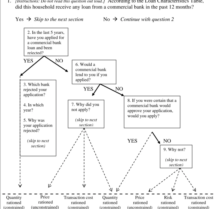
The classification of a household’s constraint status typically draws on two modules within the credit section of a household survey. Figures 1 and 2 provide examples of these two modules. Figure 1 depicts the first half of the “loan characteristic module” from the survey
of farm households in Peru that serves as the basis for the empirical analysis of Section 4. This module collects information to characterize loan contracts and is administered to households that borrowed during the recall period. Figure 2 consists of two portions. The upper portion (above the dotted line) depicts a “credit market perception module” used to describe experiences in, and perceptions of the credit market of households that did not borrow during the recall period. The bottom portion of Figure 2 does not appear in the survey but instead shows how non-borrowers’ responses lead to the classification of their constraint status and rationing mechanism.
3.2.1 Identifying supply side constrained households
We now turn to operationalizing the classification scheme described above. We begin with supply-side constrained households. Equation 6 will hold if a household received less than its desired amount of credit given terms of contracts available in the market. In identifying supply-side constrained households from survey data, it is useful to distinguish three separate groups. First, unsatisfied borrowers received a loan; however the loan amount was less than their effective demand. To identify this group, we use the response to question 11 in Figure 1, “Would you have wanted a larger loan at the same interest rate?” There are two details to note in the formulation of this question. First, the borrower is asked to compare the amount she received to the amount that she wanted. While it might seem more intuitive to compare the amount received with the amount applied for, this would be problematic since the borrower may know the lender’s supply rule and thus have only applied for the amount she qualified for. Second, the question emphasizes that the desired amount is conditional upon the interest rate. In practice, when asked without conditioning on the interest rate, respondents often interpreted the question as asking for their total working capital needs under an interest-free loan. Finally, although not essential for our present purpose of discrete categorization of constraint status, question 11 is followed by a question that asks the desired
loan size. This would then identify a point on the borrower’s demand curve and is thus useful to analyze continuous loan demand and estimate the shadow value of liquidity.
The second group is rejected applicants, who have positive effective demand but a zero credit limit. As this group did not borrow, they are identified using the credit market perception module. In Figure 2, this group responds “Yes” to question 2 which asks if they have applied and were rejected. A specific issue is the time frame specified in this question. If a household’s credit limit were time invariant, then the appropriate question would be whether or not the household has ever been rejected. If, as is more likely, the credit limit changes over time then a shorter recall period is preferable. Questions 3, 4, and 5 are not necessary for the constraint classification, however they provide quantitative information on loan demand as well as qualitative information on perceived reasons for loan rejection.
The final supply-side constrained group is “certainly-rejected” non-applicants, who had positive effective demand but did not apply for a loan because - based on past experience or their perceptions of lenders’ supply rules - they were certain their loan application would be rejected. As these are non-borrowers, we again use the perceptions module (Figure 2) to classify their constraint status. Given that they did not apply for a loan they are filtered to question 6 which asks if they believe the lender would offer a loan if they applied. If yes, then we know that the household is not supply-side constrained. If no, the enumerator continues with question 8: “If you were certain that a lender would approve your application, would you apply?” If yes, then the household is classified as constrained.5
3.2.2 Identifying demand-side constrained households
As in the case of supply-side constraints, demand-side constrained households can be either borrowers or non-borrowers. In both cases these households’ effective demand is reduced
5One specific issue to be aware of is the wording of question 8. Notice that we do not ask “would you accept a loan if you were offered one?” The reason is that the word “offered” may imply that the respondent need not incur the costs of application.
by transaction costs or risk. Our discussion here will focus on how to identify demand-side constrained non-borrowers who completely withdraw from credit markets.6
Begin at question 6 in Figure 2 which asks “would a bank lend to you if you applied?” Demand-side constrained non-borrowers are found among both those with and without per-ceived access. Households that answer “yes” to question 6 and thus believe they have credit access are then asked why they did not apply (question 7). Their response to this ques-tion, as discussed below, allows their classification as unconstrained or constrained and, if constrained, as transaction cost rationed or risk rationed. Households that answer “no” to question 6 and thus believe they have no credit access are then asked in question 8 whether they would want a loan if they were certain the lender would approve their application. As discussed above, those who say “yes” are the certainly-rejected non-applicants and are clas-sified as supply-side rationed. Those who say “no” are then asked why not in question 9 and classified as unconstrained or constrained and, if constrained, as transaction cost rationed or risk rationed.
As is hopefully clear by now, one of the main objectives of this method is to gather additional information on the credit market perceptions of non-borrowers. In particular, de-termining their constraint status requires learning why some households choose not to borrow even though they believe they qualify for a loan. In Figure 2, questions 7 and 9 elicit this information. Table 1 provides typical responses to these questions and the subsequent classi-fication of households. Recall that unconstrained non-borrowers have zero notional demand and no profitable projects that require outside financing. This group can be highly diverse including households with large endowments of productive assets and liquidity, as well as endowment-poor households with limited investment opportunities. Response C “Farming
6Ignoring demand-side constrained borrowers is likely to have little impact on the evaluation of the performance of credit markets for two reasons. First, since transaction costs typically have an important fixed component, they should have relatively little impact on effective demand for those who borrow. Second, the scope for borrowers to reduce risk by taking smaller loans is limited because collateral assets are typically lumpy and cannot be marginally adjusted, and many agricultural lenders offer boilerplate loan contracts in which loan size is a fixed multiple of area cultivated.
does not give enough to repay a debt.” is a common response from this latter type of uncon-strained household. Other frequent responses suggesting that the household is unconuncon-strained include “The interest rate is too high” and “I don’t need a loan.” Note that some responses do not lend themselves to an unambiguous classification. For example the response D “I prefer working with my own liquidity” could be consistent with both price rationing and risk rationing.7 For these responses, we suggest following a conservative approach and classifying the household as unconstrained. A demand-side constrained household, in contrast, has a Table 1: Common answers to question 7 and question 9 in Figure 2
Why did (would) you not apply for a formal loan? Constraint Status A I do not need a loan.
B The interest rate is too high. Unconstrained C Farming does not give me enough to repay a debt. (Price Rationed) D I prefer working with my own liquidity.
E I don’t want to put my land at risk.
F I do not want to be worried, I am afraid. Constrained G Formal lenders are too strict, they are not (Risk Rationed)
as flexible as informal ones.
H Formal lenders do not offer refinancing.
I The branch is too far away. Constrained J There is too much paperwork; the costs associated (Transaction Cost
with loan application are too high. Rationed)
profitable investment beyond its own liquidity that it forgoes due to risk or transaction costs. Rows E-H of Table 1 provide examples of responses associated with risk rationing. Of these, the most common response in each of the surveys we conducted was “I don’t want to risk my land.”8 Rows I and J are common responses indicating that the household was discouraged from borrowing by transaction costs. It is important to note that we interpret responses
7This response could be given by high liquidity households that are unconstrained, as well as by households with investment opportunities requiring funds beyond their own liquidity but that chose not to borrow because of risk.
8The surveys we have conducted were carried out in regions where banks exist and tend to require titled property as collateral. In areas where banks do not operate or where land cannot be used as collateral,risk rationing can still occur but is likely to manifest itself via different responses. For example, risk rationing may be quite common in villages dominated by a stereotypical moneylender who requires the borrower to put up his reputation or “knee-caps” as collateral.
E-J as indicating that households have a profitable use for credit (i.e. have positive notional demand) and have considered taking a loan, but decided no to because of risk or transaction cost.9
3.3
Issues and Challenges in Classification via Direct Elicitation
In this section, we discuss four important issues related to the use of the direct elicitation method. The first issue is conceptual and is related to the use of hypothetical and coun-terfactual questions in the perception module. The second two issues involve choices the researcher confronts in designing the questionnaire. Finally, we acknowledge the cost of this method.
3.3.1 Issue 1: Use of Hypothetical Questions
The perception module in Figure 2 uses two hypothetical questions. Question 6 asks non-applicants if they believe a bank would lend to them if they were to apply. Question 9 asks those who respond “no” to question 6 whether or not they would apply for a loan in the counterfactual situation of positive supply. There are two potential concerns associated with the use of these questions. The first concern is that the respondent may not understand the question. Until this point in the survey, the respondent has been bombarded with “factual” recall questions such as the reconstruction of farm revenues and costs. In question 6, the enumerator now asks the respondent to change gears and think about the outcome of a loan application that was not made. Similarly in question 9, the enumerator asks about the respondent’s demand for a loan that was not offered. Clearly communicating these questions is a non-trivial task. Beyond a clear phrasing of the question itself, effective use of this type
9An alternative way to identify unmet notional demand is to ask what the household would do with additional liquidity. Under this approach, followed for example by Paulson and Townsend (2004), households that say they would expand productive enterprizes (business or farm) or invest in working capital are classified as credit constrained. This question, however, does not provide sufficient information to distinguish between supply and demand-side rationing.
of hypothetical question requires careful selection and training of enumerators, who may need to step outside of the literal question in order to convey the idea.
The second issue is that identifying the constraint status of non-borrowers relies on these respondents’ perceptions of a market in which they are not currently participating. Specif-ically, identification of a binding supply constraint relies on the respondent’s perception of the lender’s willingness to offer them a loan. This perception may be incorrect. “Overly pes-simistic” respondents incorrectly believe they would be rejected, while “overly optimistic” respondents incorrectly believe their application would be accepted. For our objective of gauging the impacts of credit constraints on resource allocation, neither type of perception error is problematic. Consider two individuals with positive effective demand that are iden-tical except in their perceptions of the lender’s supply rule. The first correctly believes he faces positive supply and thus ends up with a loan and undertakes the investment project. The second, an overly pessimistic respondent, incorrectly believes he faces zero supply. As a result, he does not apply and forgoes the project. These two households would be classified as credit unconstrained and constrained, respectively. The difference in their resource allo-cations is determined by the difference in their perceived supply rule, which is captured by the direct elicitation approach, rather than the “true” supply rule. Next consider the overly optimistic respondents. The potential concern is that this method would fail to identify a binding supply constraint. This cannot happen, however, as the constraint classification of these respondents is independent of their “true” supply rule. Since they believe they could get a loan but did not apply, the lender’s true supply rule does not constrain these house-holds. Instead, they are either unconstrained or demand-side constrained, as indicated by their response to question 7 in Figure 2.
We have just argued that the classification of non-participating households as constrained or unconstrained should depend on their perception of their feasible contract set since their resource allocation depends upon the perceived instead of the “true” feasible set. Gauging the
accuracy of non-participants’ perceptions is, however, relevant to the design of appropriate policy to alleviate credit constraints. If households refrain from participating because they systematically underestimate lenders’ willingness to lend or overestimate the interest rates, risk or transaction cost of contracts that are available to them, then policies that increase the flow of information to rural households would be more appropriate than policies that seek to change the contract terms themselves.10
3.3.2 Issue 2: Definition of Loan Sectors
The second issue to consider in designing the perception module is how the lender is defined to the respondent. In practice, rural credit markets are composed of a group of heterogenous lenders including commercial banks, state banks, NGO’s and a wide range of informal lenders. Both the access rules and contract terms facing a given household may vary widely across these lenders. As a result, a household may be unconstrained with respect to one type of lender but constrained with respect to other lenders that offer more favorable contracts, for example with longer maturity or lower cost. In this case, the constraint would be binding and adversely affect the household’s resource allocation. Given this concern, lenders should be grouped into distinct sectors, or segments, of the credit market, and the language of the qualitative questions in the perceptions module should be cast with respect to these sectors. Common sectoral definitions are “formal” and “informal.” The distinction between for-mal versus inforfor-mal sectors may be based on many alternative lender characteristics. Com-mon criteria include: Is the lender regulated? Does the lender lend for profit? Is the lender
10There are several means to evaluate the accuracy of borrower’s perceptions of their feasible contract set. First, to identify the “true” supply rule, the researcher could present the household’s characteristics to a lender and ask whether or not he would be willing to offer a loan. This approach is most effective when the lender relies primarily on a quantitative evaluation of loan application such as credit scoring as opposed to more qualitative evaluations such as personal interviews. Second, the researcher can include questions in the perceptions module that ask the respondent about the interest rates and collateral requirement of specific loan products in the local market. These responses could then be compared to existing loan terms. Finally, data on credit history, degree of contact with borrowers, access to information sources such as radio, TV and internet, and other characteristics that are correlated with the accuracy of perceptions can be collected in the survey.
specialized in financial intermediation? Of course the classification need not be binary. In our study of credit markets in rural Peru, we define three sectors of regulated lending institu-tions: commercial banks, municipal banks and rural banks. While each of these institutions is regulated by the central bank, there are differences in the specific rules and regulations that apply to each type so that contract terms differ across these institutions. Notice that the questions in Figure 2 are asked with respect to commercial banks. In the survey instru-ment used in Peru these questions are then repeated for each type of bank from which the household did not borrow.
Another reason to define distinct loan sectors is to test sector specific hypotheses. For example, we might be interested in evaluating a policy that affects a certain type of in-stitution. Mushinski (1999) uses the direct elicitation approach to evaluate the impact of market oriented reforms implemented by credit unions in Guatemala on the prevalence of non-price rationing in the credit unions. We also might be interested in testing the existence of a preference hierarchy across loan sectors. Until recently, most theoretical and empirical models assumed that the formal loan sector is strictly preferred by all borrowers (Bell et al., 1997). Several authors have relaxed this assumption, arguing that informal contracts may be preferred because of lower cost (Kochar, 1997; Chung, 1995) or lower risk (Boucher and Guirkinger, forthcoming). Appropriately defining sectors allows testing of these hypotheses.
3.3.3 Issue 3: Household versus Individual Constraint
The third issue we take up is whether the credit constraint classification should be made at the household or individual level. Until now, we have couched the discussion at the household level. This approach is appropriate if we believe household resource allocation is consistent with a “unitary” household model in which endowments and income are pooled amongst household members. The qualitative questions of the perceptions module would then be addressed to the household head, who would respond for the overall household.
We assume that the head can, given the endowments and opportunities available to the household, assess the effective and notional demand of as well as the supply available to -the entire household.
If, in contrast, resources are not pooled within the household or information is not shared, then individual characteristics - including whether or not individuals are credit constrained - may impact the household’s resource allocation. In this case, each individual’s constraint status needs to be elicited and thus the perception module is applied to each adult in the household. This individual approach, while costly, is useful for testing hypotheses related to gender bias in credit access and intra-household resource allocation processes. It has been used by Diagne et al. (2001) in an exploration of credit markets in Malawi.
3.3.4 Issue 4: Cost of the Direct Elicitation Approach
While we believe there are significant benefits to the direct elicitation of credit constraints, its implementation implies additional costs. First, the application of the perception module is complex. On one hand, as seen in Figure 2, the flow control of the survey is difficult as there are many logical skips. On the other hand, enumerators need to be able to recognize uninformative answers to open questions (such as questions 7 and 9 in Figure 2), implying that they must have a basic understanding of the underlying concepts and the objectives of this module. As a result, the researcher may need to hire relatively well educated and experienced, and thus more expensive, enumerators. In addition, extended classroom and field training is required for the application of this module. Second, even with well trained enumerators, clear communication of the hypothetical questions may require repetition and additional explanation, thereby adding survey time and contributing to fatigue of both the respondent and enumerator.11
11Time and survey fatigue should be taken into account when defining the number of credit sectors to be considered.
4
Empirical Application: The Impacts of Credit
Con-straints on Agricultural Production in Peru
One of the advantages of the direct elicitation approach is that it can account for the various forms of non-price rationing that, as we argued in section 2, are likely to exist in rural credit markets. Each form of non-price rationing restricts household participation in the credit market and adversely affects investment and thus should be accounted for in any evaluation of the performance of rural credit markets. In this section we use a data set from Peru that used the direct elicitation approach to demonstrate how the consideration of demand side constraints affects our estimation of the impact of credit constraints in agricultural production.
Our impact measure is the estimated increase in the value of production in the study area that would occur if the credit constraints of households observed as constrained were alleviated. We estimate this impact using two alternative definitions of credit constraint. The first definition, which we call the “restrictive” definition, classifies as credit constrained only those households that are supply-side constrained. The second definition, which we call the “comprehensive” definition, classifies a household as constrained if it is constrained from either the supply or demand side. There are two ways by which this difference in definition can lead to differences in the predicted impact. First, by definition, at least as many households will be classified as constrained under the comprehensive definition than the restrictive definition. Second, the magnitude of the predicted impact of relaxing a given household’s credit constraint may differ if the composition of the constrained group changes systematically with the constraint definition.
4.1
Data and Context
The data come from a survey administered to farm households in 1997 and again in 2003 in the department of Piura, on Peru’s north coast. A random sample of farm households was drawn from the comprehensive lists maintained by the irrigation commissions (comisiones de regantes). The sample is representative of irrigated, commercial agriculture in the region. Of the original 547 households surveyed in 1997, 499 were resurveyed in 2003. The empirical analysis in this section is based on the 442 households that farmed in both years.
The survey was designed to measure the incidence and impacts of credit constraints in the formal credit sector which, in Piura, consists of three types of institutions: commercial banks, municipal banks (cajas municipales) and rural banks (cajas rurales). A non-borrower perceptions module similar to the one in Figure 2 was repeated for each of these three insti-tution types to which the household did not apply.12 A loan characteristics module captured details of all loans taken from either formal or informal sources. Based on the method described in Section 3, we used these two modules to classify households as constrained or unconstrained in the formal sector according to both the restrictive and comprehensive definitions of credit constraint.
The first column of Table 2 gives the frequency of credit constraints for the sample pooled across the two years under the two alternative definitions. As 23% of households were quantity rationed, this is also the frequency of constrained households using the restrictive definition. Under the comprehensive definition, the frequency of credit constraints increases to 49% reflecting the inclusion of risk and transaction cost rationed households. The second and third columns give the percentage of households that borrowed from the formal and informal sectors respectively.13 As seen in the first row, 51% of price rationed households
12A household is classified as unconstrained in the formal sector if it was unconstrained with respect to any of the three types of institutions.
13The informal sector in Piura consists primarily of rice mills, input supply stores, grain traders, unregu-lated credit programs run by NGO’s and local government, and family and friends.
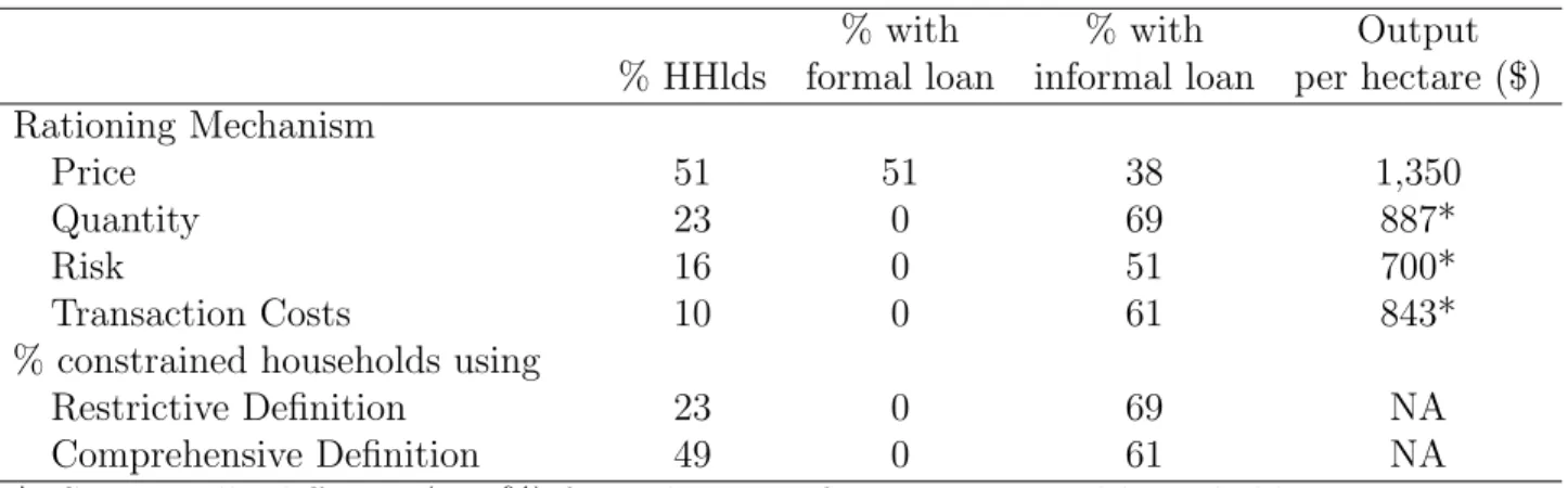
Table 2: Credit use and productivity by rationing mechanism
% with % with Output % HHlds formal loan informal loan per hectare ($) Rationing Mechanism
Price 51 51 38 1,350
Quantity 23 0 69 887*
Risk 16 0 51 700*
Transaction Costs 10 0 61 843* % constrained households using
Restrictive Definition 23 0 69 NA Comprehensive Definition 49 0 61 NA *: Statistically different (at 5%) from the mean for price rationed households.
borrowed in the formal sector while 38% borrowed in the informal sector. The second and third rows show that, as expected, a larger percentage of households that were non-price rationed in the formal sector borrowed from the informal sector. If loan terms were similar across sectors, then the high rates of participation in the informal sector would suggest that formal constraints would have little impact on household resource allocation. Informal loans are not, however, close substitutes to formal loans as they are significantly smaller, have higher interest rates, and shorter terms than their formal counterparts.14 The last column of Table 2 provides descriptive evidence that each form of non-price rationing adversely affects farm resource allocation. Compared to price rationed households, the value of production per-hectare is significantly lower for each of the three types of non-price rationed households, in spite of the presence of an active informal sector. This column also suggests the importance of the credit constraint definition. Under the restrictive definition, risk and transaction cost rationed households are grouped together as unconstrained along with the price rationed households. Yet based on their productivity, their resource allocation looks much more similar to the quantity rationed households, suggesting that the impact of credit constraints would be larger if the comprehensive definition is used.
14Boucher and Guirkinger (forthcoming) provide a detailed comparison of loan terms across sectors for the study area as well as for other regions in Latin America.
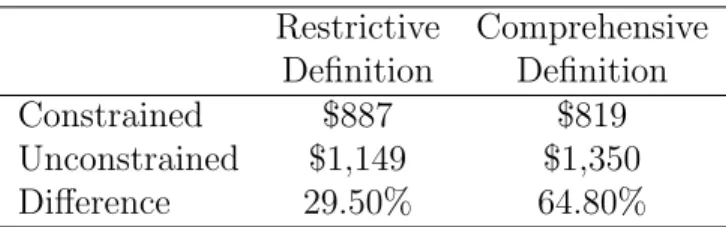
Table 3 compares mean productivity levels for constrained and unconstrained households under the two definitions and indeed suggests that the impact of credit constraints is greater under the comprehensive definition. The productivity differential between unconstrained and constrained households increases from 29.5% to 64.8% when risk and transaction cost rationed households are included in the constrained group.
Table 3: Credit constraints and productivity Restrictive Comprehensive
Definition Definition Constrained $887 $819 Unconstrained $1,149 $1,350 Difference 29.50% 64.80%
The descriptive evidence presented above is suggestive of two things. First, credit con-straints appear to have a large negative impact on production in Piura. Second, the mag-nitude of the impact differs considerably depending on how credit constraints are defined. Whether or not we can attribute these impacts to credit constraints per se, however, is not certain since we have not controlled for other factors that affect farm productivity and that may be correlated with households’ credit constraint status. The next section develops an econometric model that controls for both observed and unobserved determinants of farm productivity and thus allows us to isolate the impact of credit constraints.
4.2
Econometric Model
Consider the following linear specification of farm productivity:
yit = α + βCit+ γZit+ ηi + εit (8)
The dependent variable, yit, is the per-hectare value of farm output for household i in period
in period t and zero if unconstrained. Zit is a vector of time varying household and farm
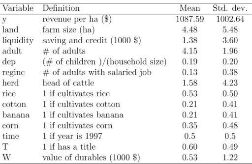
characteristics that impact productivity. Included in Zit are: the household’s endowments
of land, liquidity and labor; the households dependency ratio; the availability of regular wage earners; the size of the household’s cattle herd, and dummy variables indicating the household’s crop mix. The definitions, means and standard deviations of all variables are reported in Table 4. The household fixed effect, ηi, captures the impact of time invariant
household characteristics affecting productivity, while α, β, and γ are parameters to be estimated. Finally, εit is a mean zero error term.
We are primarily interested in β, which gives the impact of being credit constrained on farm productivity. In order to see how the definition of the credit constraint influences β we estimate equation 8 twice - first using the restrictive definition then using the comprehensive definition. In estimating β, we face two potential sources of bias. First, the household fixed effect is unobserved and potentially correlated with the other regressors. We estimate equation 8 using first differences and thereby eliminate this potential source of bias. Second, unobserved time varying factors such as shocks to land quality or health may be correlated with both productivity and the household’s credit constraint status. To address this potential source of endogeneity, we use an instrumental variable approach. We use two instruments for the household’s credit constraint status. The first is Tit, which takes value one if the
household has a registered property title and zero otherwise. Possession of a title reduces the probability of being constrained as titled land is the primary form of collateral required by formal lenders.15 The second instrument, W
it, is the value of the household’s consumer
durables which reduces the probability of being constrained for two reasons. First, durables are taken as a signal of repayment capacity by lenders. Second the value of durables is an indicator of wealth which, under the assumption of decreasing absolute risk aversion, is
15The literature on property rights (Besley 1995) suggests that a title may also have a direct impact on productivity if title augments tenure security which, in turn, leads to greater investment. In Piura, a registered title is unlikely to have this direct tenure security effect on productivity because non-titled farmers possess alternative documents recognized by local authority.
positively correlated with the household’s willingness to take on risky loan contracts.
Table 4: Definition and Summary Statistics of Variables included in the Estimation Variable Definition Mean Std. dev.
y revenue per ha ($) 1087.59 1002.64 land farm size (ha) 4.48 5.48 liquidity saving and credit (1000$) 1.38 3.60 adult # of adults 4.15 1.96 dep (# of children )/(household size) 0.19 0.20 reginc # of adults with salaried job 0.13 0.38 herd head of cattle 1.58 4.23 rice 1 if cultivates rice 0.53 0.50 cotton 1 if cultivates cotton 0.21 0.41 banana 1 if cultivates banana 0.21 0.41 corn 1 if cultivates corn 0.35 0.48 time 1 if year is 1997 0.5 0.5 T 1 if has a title 0.60 0.49 W value of durables (1000$) 0.53 1.22
The estimation is carried out in STATA using first two-stage least square (2SLS) with ro-bust standard errors and then limited information maximum likelihood (LIML) with roro-bust standard errors. We follow Staiger and Stock (1997) and prefer LIML to 2SLS as the F-test for the statistical significance of the instruments in the first stage suggests that our instru-ments are weak.16 For each estimation, we perform the Hansen J test for overidentification.
It suggests that, in all cases, our instruments are valid in the sense of being orthogonal to the disturbance term ε.17
4.3
Estimation Results and Discussion
Table 5 presents results of the estimations. The first two columns report the 2SLS and LIML results under the restrictive definition of credit constraints, while the last two columns report
16The first stage F-test is 3.81 which is well below the threshold of 10 for weak instruments. As suggested by Staiger and Stock (1997) LIML limits the biases in point estimates introduced by weak instruments.
17Results are reported in the last row of Table 5. The null hypothesis of the test is that the instruments are independent of ε, failing to reject the null hypothesis therefore suggests that the set of instrument is valid.
the results under the comprehensive definition. Under both definitions, credit constraints
Table 5: Parameter estimates and standard errors (in parentheses) Restrictive Comprehensive
definition definition Variable 2SLS LIML 2SLS LIML C −740.58∗ −798.84∗∗∗ −867.32∗∗ −903.30∗∗∗ (−391.53) (−300.81) (414.50) (309.41) land −193.70∗∗∗ −195.03∗∗∗ −203.81∗∗∗ −204.94∗∗∗ (40.69) (29.16) (45.18) (32.35) liquidity 16.27 15.57 9.85 9.21 (13.66) (9.71) (14.29) (10.25) adult 14.96 17.03 12.70 13.70 (29.45) (21.49) (29.03) (20.92) dep 291.18 306.21∗ 205.60 209.98 (255.25) (185.56) (231.33) (165.63) reginc 81.38 83.91 96.94 98.92 (124.45) (88.90) (133.51) (95.38) herd 24.04∗∗ 23.92∗∗∗ 34.24∗∗∗ 34.61∗∗∗ (11.55) (8.23) (12.03) (8.61) rice 524.94∗∗∗ 529.88∗∗∗ 457.10∗∗∗ 456.89∗∗∗ (118.08) (84.68) (117.32) (83.60) cotton −249.47∗∗ −243.3∗∗∗ −182.53 −176.51∗ (105.98) (77) (130.21) (94.74) banana −95.46 −97.06 −24.53 −22.43 (209.66) (149.38) (207.91) (147.96) corn −31.56 −22.39 −70.46 −67.24 (102.30) (75.69) (91.92) (66.48) time −480.73∗∗∗ −494.21∗∗∗ −382.53∗∗∗ −385.56∗∗∗ (106.07) (79.85) (67.05) (48.40) Hansen J stat χ2 0.65 0.58 2.02 1.58 p value 0.42 0.44 0.16 0.21
***, **, *: parameter estimate significant at 1%, 5% and 10%, respectively
have a negative and significant impact on farm productivity, regardless of the estimation method. As we prefer the LIML estimations due to the weakness of our instruments, we will now focus the discussion on those results. Consistent with our expectation, the parameter estimate ˆβ is larger when the comprehensive definition of credit constraints is used instead
of the restrictive definition. In particular, the results under the restrictive definition suggest that relaxing credit constraints would raise the value of production per hectare by $799 on average, while under the comprehensive definition, relaxing credit constraint would raise productivity by 13% more, or $903 on average.
We now use these results to generate an estimate of the percentage increase in the total value of agricultural production if all credit constraints were relaxed in the region. To do so, we compute ∆, defined as follows:
∆ = P
j[E(yj|C = 0) ∗ landj − E(yj|C = 1) ∗ landj]
P i P tyitlandit = ˆ βP jlandj P i P tyitlandit (9)
where j ∈ J , and J is the set of credit constrained observations in the pooled sample. The numerator gives the predicted change in the total value of production if the credit constraints of households observed to be constrained were relaxed. The denominator gives the total observed value of production for all households in the sample. We find that alleviating credit constraints would raise regional output by 18.4% under the restrictive definition and by 44.7% under the comprehensive definition. In this example, accounting for transaction cost and risk rationing leads to a measure of impact that is over twice as large as obtained under the restrictive definition. Two elements contribute to this sharp increase. First, as mentioned above, the parameter estimate ˆβ is 13% larger under the comprehensive definition. Second, transaction cost and risk rationed households control 24% of sample land. When they are included in the constrained group, the percentage of land controlled by constrained farmer increases from 20% to 44% of total land in the sample.18
18Guirkinger and Boucher (2006) use the same data to estimate the impacts of credit constraints using an endogenous switching regression framework that allows all coefficients to differ across constrained and unconstrained households. To keep the presentation here more streamlined, we chose to estimate the simpler, single equation model given by equation 8. The sign and magnitude of the impact estimates in that paper are similar to the impact measure here using the comprehensive credit constraint definition.
5
Conclusion
The potential for non-price rationing in credit markets raises important concerns for devel-opment policy. Equilibrium rationing also raises challenges to empirical analyses of credit markets. One of the main challenges is to understand why non-borrowing households do not participate in the credit market. We have outlined a strategy, based on a series of questions that elicit respondents’ experience in and perceptions of the credit market, to distinguish between non-borrowing households that have unmet notional demand versus those that do not. As the former group’s resource allocation is adversely affected by their terms of ac-cess to the credit market, they should be considered credit constrained. In our empirical application we found that neglecting demand-side constraints would result in a significant underestimation of both the frequency and impacts of credit constraints in rural Peru.
An important contribution of the direct elicitation approach is that it permits the iden-tification of the “rationing mechanism” underlying credit constraints. While each form of non-price rationing reduces efficiency and income, they each suggest different policy re-sponses. The presence of quantity rationing indicates that some households that are willing to bear both the costs and risks of loan contracts are involuntarily shut out of the credit market by lenders. Relaxing this type of binding supply-side constraint requires policies such as land titling or property rights reforms that make households’ assets more viable to lenders as collateral or investment in credit bureaus or other institutions that enhance the flow of information so that lenders can more easily identify high quality borrowers. A significant presence of households that are constrained by transaction cost and risk rationing indicates the presence of different types of problems. These households voluntarily refrain from participating even though they have access to loans that, considering the interest costs, would raise their expected income. The types of policies mentioned above to relax supply-side constraints would not relax the constraints facing these households. Instead, policies
addressed at streamlining legal processes for registering and enforcing loan contracts or that provide a means of insuring households against production, price or health risk would be more appropriate.
3. Ty pe of l en d er 4. Wh ic h h ous ehol d me m b er receive d the loa n ?? 5. W h at was the lo an u sed fo r? 8. W h at was the v alu e o f inp uts y ou receive d? 12. Ho w m u ch m o re w o u ld y ou ha ve wan ted? list of lo an s 2. Na m e o f t h e len d er See bel o w Ind iv idu al code See below 6. For wha t crop di d y ou req u es t the loan? 7. Ho w was th e lo an di sbur se d ? 1. O n ly i n c a sh >> 11 2 .Onl y in kind >> 8 3. B o th in ca sh an d kind> > 8 Am oun t Mn 1. S /. 2. $ 9. If y ou w o u ld ha ve b oug ht th es e inpu ts in cas h , w o u ld y ou ha ve pai d : 1. M o re >> 10 2.Less >> 10 3.The same >> 11 10. Wh at w o u ld be the % dif fere n ce if y ou w o u ld ha ve b oug ht them in cas h? 11. W ould y ou ha ve wante d a lar g er lo an at th e sa m e in tere st ? 1.ye s >> 12 2 .no >>14 Am oun t Mn. 1. S /. 2. $ 13. W h y did y ou no t receive wh at y ou wan ted? See belo w 01 02 Co des Qu est ion 3 Qu est ion 5 Qu est ion 13 Fo rm al 1 .Co mmer cial ba nk 2 .Rur a l ban k 3. M u nic ipa l ba nk S emi -F o rma l 5 .Go vern ment pro g ramo 6 .Coop er at ive 7. P rod uce r a ssoc iat ion 8 .NGO In fo rm al 9 . Inp u t supp li er 10. R ice m ill 11.T extile com p any 12. G ra in tr a d er 13. G roce ry st o re 14. R ela ti ve, fr ie nd 1 6 .O th er_ ___ ___ 1 .To b u y in put s >> 6 2 . To i n stal l p er enia l cr ops >> 6 3 . T o bu y a g ri cu lt u ra l ma te rial . >> 7 4 . Ot her a g ri cult ura l in vest men t _ ___ ___ _>> 7 5. S ta rt a new bu si ne ss >> 7 6 . Sp en di ng r elat ed to th e bu si ne ss >> 7 7 . To b u y ma teri al for th e bu si ne ss >> 7 8. E d uca ti o n > > 7 9 .Cons u m p tio n>> 7 10H ou se im p ro vem en t>> 7 11B uy o r bu il d a h o u se>> 7 1 2 .O th er_ ___ ___ ____ __ >> 7 1 . La ck of coll at er al 2 . Pr oj ect not pr ofi tab le enou gh 3 . Lendi ng pol icy of th e ins ti uti on 4 .ot her__ ___ ___ ____ ___ ___ 14. D o y ou ha ve t o pay inte res t on th is l o an ? 15. W h at is th e i n te re st r ate ? 16. W h en d id y ou recie v e this loa n ? 17. H o w oft en do y ou pa y in st al lm ents ? 18. Ho w m u ch do y ou pay in each in st al lm ent ? 19. Ho w m an y in st al lem ents w il l y ou pay in t o ta l ? 20. In to tal , h o w m u ch w ill y ou pay to ca nce l t h is loa n ? 21. W h en w il l y ou fi ni sh pay ing ? rate tim e peri od m onth y ear Am o un t Mn. Am out n Mn. Mo nt h Y ear list o f lo an s 1. Y es>> 15 2.No>> 16 (%) 1 .da il y 2.week ly 3. m o nt hl y 4. A n nu a ly 5. O ther _ ___ ___ (1-12) 1d a ily 2.week ly 3. m o nt hl y 4 .ann ua ly 5. o n ce at th e en d>> 20 6 . it is no t fi xed>>2 0 1. S /. 2. $ 1. S /. 2. $ 1-1 2 0 1 0 2 Figur e 1: Sa mple lo an chara cteristic mo dule (first 21 q ue stio ns)
2. In the last 5 years, have you applied for a commercial bank loan and been rejected? 3. Which bank rejected your application? 4. In which year? 5. Why was your application rejected? (skip to next section) 6. Would a commercial bank lend to you if you applied?
7. Why did you not apply?
(skip to next section)
8. If you were certain that a commercial bank would approve your application, would you apply?
YES NO 9. Why not? (skip to next section) YES NO YES NO
1. [Instructions: Do not read this question out loud.] According to the Loan Characteristics Table, did this household receive any loan from a commercial bank in the past 12 months?
Yes Æ Skip to the next section No Æ Continue with question 2
Quantity rationed (constrained) Price rationed (unconstrained) Transaction cost rationed (constrained) Quantity rationed (constrained) Price rationed (unconstrained) Risk rationed (constrained) Transaction cost rationed (constrained)
Figure 2: Sample non-borrower perceptions module
References
Aghion, P. and Bolton, P. (1997). A theory of trickle-down growth and development. Review of Economic Studies, 64(2):151–172.
Banerjee, A. and Duflo, E. (2004). Do firms want to borrow more? testing credit constraints using a directed lending program. C.E.P.R. Discussion Papaer 2681.
Banerjee, A. and Newman, A. (1993). Occupational choice and the process of development. Journal of Political Economy, 101(2):274–298.
Barham, B., Boucher, S., and Carter, M. (1996). Credit constraints, credit unions, and small scale-producers in Guatemala. World Development, 24(5):792–805.
Bell, C., Srinivasan, T., and Udry, C. (1997). Rationing, spillover, and interlinking in credit markets: The case of rural Punjab. Oxford Economic Papers, 49:557–585.
Bester, H. (1987). The role of collateral in credit markets with imperfect information. Eu-ropean Economic Review, 31:887–899.
Boucher, S., Carter, M., and Guirkinger, C. (2005). Risk rationing and activity choice. Working Paper 05-010, Department of Agricultural and Resource Economics, University of California - Davis.
Boucher, S. and Guirkinger, C. (Forthcoming). Risk, wealth and sectoral choice in rural credit markets. American Journal of Agricultural Economics.
Carter, M. and Barrett, C. (2006). The economics of poverty traps and persistent poverty: an asset-based approach. The Journal of Development Studies, 42(2):178–199.
the impact of property rights on the quantity and composition of investment. American Journal of Agricultural Economics, 85(1):173–186.
Chung, I. (1995). Market choice and effective demand for credit: The roles of borrower transaction costs and rationing constraints. Journal of Economic Development, 20(2):23– 44.
DeMel, S., McKenzie, D., and Woodruff, C. (2006). Returns to capital. mimeo.
Diagne, A., Zeller, M., and Sharma, M. (2001). Access to credit and its impact on welfare in Malawi. Research Report 116, IFPRI, Washington.
Eswaran, M. and Kotwal, A. (1989). Credit as insurance in agrarian economies. Journal of Development Economics, 31:37–53.
Eswaran, M. and Kotwal, A. (1990). Implications of credit constraints for risk behavior in less developed economies. Oxford Economic Papers, 42:473–482.
Feder, G., Lau, L. J., Lin, J. Y., and Luo, X. (1990). The relation between credit and productivity in Chinese agriculture: A model of disequilibrium. American Journal of Agricultural Economics, 72(5):1151–1157.
Foltz, J. (2004). Credit market access and profitability in Tunisian agriculture. Agricultural Economics, 30:229–240.
Guirkinger, C. and Boucher, S. (2006). Credit constraints and productivity in Peruvian agriculture. mimeo.
Guirkinger, C. and Trivelli, C. (2006). Limitado financiamiento formal para la peque˜na agricultura: solo un problema de falta de oferta? Debate Agrario, 40.
Hoff, K. and Stiglitz, J. (1990). Imperfect information and rural credit markets: Puzzles and policy perspectives. World Bank Economic Review, 5:235–250.
Jappelli, T. (1990). Who is credit constrained in the U.S. economy? Quarterly Journal of Economics, 105(1):219–234.
Karlan, D. and Zinman, J. (2006). Expanding credit access: using randomized supply decisions to estimate the impacts. Mimeo. Yale University.
Kochar, A. (1997). An empirical investigation of rationing constraints in rural credit markets in India. Journal of Development Economics, 53:339–371.
Mushinski, D. (1999). An analysis of loan offer functions of banks and credit unions in Guatemala. Journal of Development Studies, 36(2):88–112.
Paulson, A. and Townsend, R. (2004). Entrepreneurship and financial constraints in Thailand. Journal of Corporate Finance, 10:229–262.
Petrick, M. (2004). A microeconometric analysis of credit rationing in the Polish farm sector. European Review of Agricultural Economics, 31:23–47.
Udry, C. and Conning, J. (2005). Rural financial markets. In Evenson, R., Pingali, P., and Schultz, T., editors, Handbook of Agricultural Economics, volume III, chapter 14. Elsevier Science, North Holland, Amsterdam.
Zimmerman, F. and Carter, M. (2003). Asset smoothing, consumption smoothing and the reproduction of inequality under risk and subsistence constraints. Journal of Development Economics, 71:233–260.