HAL Id: hal-01457989
https://hal.archives-ouvertes.fr/hal-01457989
Submitted on 6 Feb 2017
HAL is a multi-disciplinary open access
archive for the deposit and dissemination of
sci-entific research documents, whether they are
pub-lished or not. The documents may come from
teaching and research institutions in France or
L’archive ouverte pluridisciplinaire HAL, est
destinée au dépôt et à la diffusion de documents
scientifiques de niveau recherche, publiés ou non,
émanant des établissements d’enseignement et de
recherche français ou étrangers, des laboratoires
Edge-intersection graphs of grid paths: The
bend-number
Daniel Heldt, Kolja Knauer, Torsten Ueckerdt
To cite this version:
Daniel Heldt, Kolja Knauer, Torsten Ueckerdt.
Edge-intersection graphs of grid paths:
The bend-number.
Discrete Applied Mathematics,
Elsevier,
2014,
167,
pp.144 - 162.
Edge-intersection graphs of grid paths:
the bend-number
Daniel Heldt1, Kolja Knauer2,∗, Torsten Ueckerdt3,∗∗
Abstract
We investigate edge-intersection graphs of paths in the plane grid, regarding a parameter called the bend-number. I.e., every vertex is represented by a grid path and two vertices are adjacent if and only if the two grid paths share at least one grid-edge. The bend-number is the minimum k such that grid-paths with at most k bends each suffice to represent a given graph. This parameter is related to the interval-number and the track-number of a graph. We show that for every k there is a graph with bend-number k. Moreover we provide new upper and lower bounds of the bend-number of graphs in terms of degeneracy, treewidth, edge clique covers and the maximum degree. Furthermore we give bounds on the bend-number of Km,nand determine it exactly for some pairs of mand n. Finally, we prove that recognizing single-bend graphs is NP-complete, providing the first such result in this field.
1. Introduction
Golumbic, Lipshteyn and Stern [14] introduced edge-intersection graphs of
paths on a grid (EPG graphs), a concept arising from VLSI grid layout
prob-lems [6]. A simple graph G is an EPG graph, if there is an assignment of paths in the plane grid to the vertices, such that two vertices are adjacent if and only if the corresponding paths intersect in at least one grid-edge. The assignment is then called an EPG representation of G. EPG graphs generalize
edge-intersection graphs of paths on degree 4 trees as considered by Golumbic,
Lipshteyn and Stern in [13]. In [14] it is shown that every graph is an EPG graph, however a certain parameter of EPG representations has awoken some interest. The bend-number b(G) of G is the minimum k, such that G has an EPG representation, with each path having at most k bends. Here a bend of a
grid path is a switch in its direction between horizontal and vertical. Figure 1
shows an EPG representation of K3,10 where each path has at most two bends,
∗
Research was supported by the DFG as a GraDR EUROGIGA project.
∗∗
Research was supported by GraDR EUROGIGA project No. GIG/11/E023.
1
Technische Universit¨at Berlin
2
Universit´e Montpellier 2
3
hence b(K3,10) ≤ 2. Generally, a graph G with b(G) ≤ k is referred to as a k-bend
graph.
Figure 1: A 2-bend representation of K3,10.
Remark. Most of the literature concerning this topic, including [3, 4, 14], is considering Bk, the class of k-bend graphs. Clearly b(G) ≤ k just paraphrases G∈ Bk. However, we prefer to use b(G) rather than Bk.
Graphs with bend-number at most 1, called single-bend graphs, already aroused interest in several respects, as seen in [2, 7, 14, 31]. In [3, 4] it has been shown that the bend-number of a graph can be arbitrarily large. Hence it is interesting to determine graphs or graph classes with bounded bend-number. Asinowski and Suk [3] give bounds on the bend-number of complete bipartite graphs. In [22] it is shown that b(G) ≤ 4 for every planar G, b(G) ≤ 3 for planar graphs with tree-width at most 3 and that this is best-possible, and that b(G) ≤ 2 for every G with tree-width at most 2, which includes outerplanar graphs and is best-possible due to an example of Biedl and Stern [4]. Biedl and Stern [4] also give upper bounds on b(G) in terms of treewidth, pathwidth, degeneracy and maximum degree of G.
Comparing parameters
Interval graphs are intersection graphs of intervals on the real line. Every
vertex is associated with an interval, in such a way that two intervals overlap if and only if the corresponding vertices are adjacent. This subject has been extended to intersection graphs of systems of intervals in two ways:
In a k-interval representation of a graph G every vertex is associated with
a set of at most k intervals on the real line, such that vertices are adjacent iff any of their intervals intersect. The interval-number i(G) is then defined as the minimum k, such that G has a k-interval representation, see [21].
In a k-track representation of a graph G there are k parallel lines, called
tracks. Every vertex is associated with one interval from each track. Again
vertex adjacency is equivalent to interval intersection and the track-number t(G) is the minimum k, such that G has a k-track representation, see [19].
For emphasis we repeat:
A k-bend representation is an EPG representation where each vertex is
represented by a path with at most k bends, i.e., at most k + 1 segments. In this sense such a representation associates every vertex with at most k+ 1 intervals. The bend-number b(G) is the minimum k, such that G has a k-bend representation.
Thus, the bend-number is yet another way to measure how far a graph is from being an interval-graph. Note that interval graphs are precisely the graphs with i(G) = t(G) = b(G) + 1 = 1.
Now, b(G) can be set in relation to i(G) and t(G): b(G) is only a constant factor away from i(G) and t(G). Consecutive intervals representing a vertex in a k-interval representation may be connected by introducing three segments such that they form a grid-path. It is easy to see, that a k-track representation can be transformed into a k-interval representation, by putting the tracks on a single line, i.e., i(G) ≤ t(G). Thus one gets b(G) ≤ 4(i(G) − 1) ≤ 4(t(G) − 1). On the other hand the grid-lines of a k-bend representation can be stringed together on a single line, i.e., i(G) ≤ b(G) + 1. We believe that no such bound exists for the track-number.
Conjecture 1. There is no function f such that t(G) ≤ f (b(G)) for all G
and equivalently no such function exists replacing b by i. We suspect that the line graph of Kn is a good candidate for showing this, i.e., that this family has
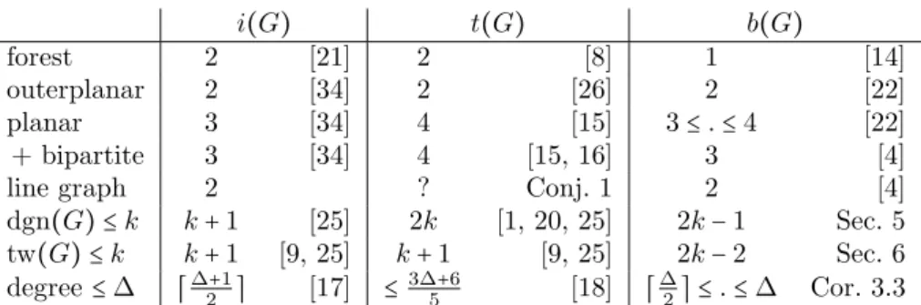
unbounded track-number, whereas in [4] it is shown that it has bend-number at most 2. i(G) t(G) b(G) forest 2 [21] 2 [8] 1 [14] outerplanar 2 [34] 2 [26] 2 [22] planar 3 [34] 4 [15] 3 ≤ . ≤ 4 [22] + bipartite 3 [34] 4 [15, 16] 3 [4]
line graph 2 ? Conj. 1 2 [4]
dgn(G) ≤ k k+ 1 [25] 2k [1, 20, 25] 2k − 1 Sec. 5 tw(G) ≤ k k+ 1 [9, 25] k+ 1 [9, 25] 2k − 2 Sec. 6 degree ≤ ∆ ⌈∆2+1⌉ [17] ≤3∆5+6 [18] ⌈∆2⌉ ≤ . ≤ ∆ Cor. 3.3
Table 1: Some graph classes and their maximum interval-number, track-number and bend-number. Here dgn(G) and tw(G) denotes the degeneracy and treewidth of G, respectively.
Many extremal questions about interval-numbers and track-numbers have been studied. In Table 1 we have listed some considered graph classes and the maximum i(G), t(G) and b(G) + 1 among all G in this class. In the last two columns (corresponding to the track-number and the bend-number) some values remain unknown, yielding several interesting problems to attack.
Our Results
In Section 3 we bound the bend-number of a graph in terms of its global
and local clique covering number. This generalizes the bound for line graphs from [4] and improves it for line graphs of bipartite graphs. As a corollary we obtain that b(G) ≤ ∆ + 1 where ∆ denotes the maximum degree of G, which improves the previous bound of 2⌈∆+12 ⌉ + 1 from [4].
In Section 4 we present two lower bounds on the bend-number of the
complete bipartite graph Km,n. From the first we obtain that b(Kn,n) = ⌈n
2⌉, which in particular proves that for every k there is a k-bend graph that is not a(k−1)-bend graph. This confirms a conjecture of [14] and has been shown for even k in [4]. With our second lower bound we improve the bound from [4] on the minimal n for which b(Km,n) = 2m − 2. Moreover we show that this new bound is almost tight, disproving a conjecture of Biedl and Stern [4].
In Section 5 we prove that b(G) ≤ 2dgn(G) − 1 for all graphs G, where
dgn(G) denotes the degeneracy of G. This was suspected in [4], where the authors prove a bound of 2dgn(G)+1. We additionally show that our new bound is best-possible even for bipartite graphs.
In Section 6 we prove that b(G) ≤ 2tw(G)−2 for all graphs G, where tw(G)
denotes the treewidth of G, generalizing the known b(Km,n) ≤ 2m − 2 [4]. This improves a result of Biedl and Stern [4] who achieve the same bound, but with pathwidth instead of treewidth. Our bound is best-possible.
In Section 7 we present the first hardness result in the field of EPG graphs.
In particular we prove that recognizing single-bend graphs is NP-complete, answering a question that has been frequently asked [4, 14]. The recogni-tion of k-bend graphs for k ≥ 2 remains open.
2. Preliminaries
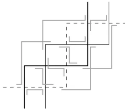
We consider simple undirected graphs G with vertex set V(G) and edge set E(G). An EPG representation is a set of finite paths {P(v) ∣ v ∈ V (G)}, which consist of consecutive edges of the rectangular grid in the plane, such that {v,w} ∈ E(G) if and only if P(v)∩P(w) contains a grid-edge. In particular two paths representing non-adjacent vertices may intersect in grid-points. A bend of P(v) is a point of P(v), where a horizontal grid-edge of P(v) is followed by a vertical grid-edge of P(v).
The set of grid-edges between two consecutive bends or the first (last) bend and the start (end) of P(v) is called a segment. So a k-bend path consists of k+ 1 segments, each of which is either horizontal or vertical. A subsegment is a connected subset of a segment. Two horizontal subsegments in an EPG representation see each other if there is a vertical grid-line intersecting both subsegments. Similarly, two vertical subsegments see each other if there is a horizontal grid-line intersecting both. We say that a subsegment s ⊂ P(v)
displays v if the grid-edges on s are exclusively in P(v) and in no other path.
Similarly, a segment s ⊂ P(v) ∩ P(w) displays the edge {v,w} if every grid-edge of s is only contained in P(u) ∩ P(v) and not element of any other path.
Two special types of paths appear more frequently in the paper: A path P is a staircase if going along P we see alternating left turns and right turns, and a path P with an even number of bends is called a snake if we see alternating two left turns and two right turns.
For a set S of horizontal (respectively vertical) subsegments in an EPG representation that pairwise see each other we say that a grid path P connects S if P is a snake and every horizontal (respectively vertical) segment of P is contained in a different subsegment from S. More formally, there are two vertical (respectively horizontal) grid-lines ℓ1 and ℓ2 that intersect all subsegments in S and contain all vertical (respectively horizontal) segments of P , while each vertical segment of P is completely contained in a different subsegment from S. A grid path that connects S has exactly 2∣S∣ − 2 bends.
3. Edge Clique Covers
In this section we present a general method to represent any graph with a number of bends depending on an edge clique cover. More precisely, letC be the graph class of cliques and their disjoint unions. A collection C1, . . . , Cℓ of members ofC is an edge clique cover of G if each Ci can be mapped into G by an injective homomorphism, so that each edge of G is in the image of at least one Ci. Denote by clg(G) the global clique covering number, i.e., the minimum number of elements ofC needed for an edge clique cover of G. Moreover denote by clℓ(G) the local clique covering number, i.e., the minimum over all edge clique covers of G of the maximum number of members containing the same vertex of Gin their image. It is easy to see that clℓ(G) ≤ clg(G).
Theorem 3.1. Let G be a graph. Then b(G) ≤ clg(G) − 1.
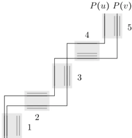
Proof. Let Cifor 1 ≤ i ≤ k = clg(G) denote the members of the edge clique cover, extended by 1-cliques, such that each Ci covers all vertices. We use staircases with k − 1 bends to represent the vertices of G. Every Ci consists of vertex disjoint cliques Si(j) covering all vertices for 1 ≤ j ≤ ℓi. We associate with every vertex v the vector xv with xv(i) = j iff v ∈ Si(j). We set ℓ−1 = 0 and ℓ0= 1 and xv(0) = 0. The path P(v) is defined by the coordinates of its start point, bends and end point (p1, p2, . . . , pk, pk+1). Define pi ∶= (xv(i) + i − 1 + ∑(i−1)/2
j ℓ2j−1, xv(i − 1)) if i is odd and (xv(i − 1),xv(i) + i − 1 + ∑ (i−2)/2
j ℓ2j) if i is even.
Along the i-th segment, two paths run through the same grid-line if and only if the corresponding vertices are in the same clique in Ci. Afterwards, they bend eventually at different points in order to meet the line corresponding to the clique containing them in Ci+1, respectively. See Figure 2 for an illustration.
1 2
3
4 5
P(u) P(v)
Figure 2: A (k −1)-bend representation based on an edge clique cover with k unions of cliques: The gray blocks correspond to the members of the clique cover. Every clique in Ciis assigned
a grid-line within the i-th block. Paths are inserted as demonstrated by P (u) and P (v) according to the cliques they are in.
Example. As illustrated in Figure 3, every induced subgraph of the triangular plane grid has global clique covering number at most 3. We conclude that the bend-number of the triangular plane grid and all of its induced subgraphs is at most 2.
Figure 3: A subgraph G of the triangular plane grid covered by 3 unions of cliques. Hence b(G) ≤ 2.
Line graphs of bipartite graphs can be covered by two unions of cliques corresponding to the stars of the vertices of the first and the second bipartition class, respectively.
Corollary 3.2. Line graphs of bipartite graphs are single-bend graphs.
A proper edge coloring of G is a special case of an edge clique cover of G as in Theorem 3.1. Hence the bend-number b(G) is bounded by the edge chromatic number χ′(G). This implies a strengthening of a result of [4] concerning the maximal degree ∆ of G:
Corollary 3.3. If χ′(G) denotes the edge chromatic number of G, then b(G) ≤ χ′(G) − 1. In particular Vizing’s Theorem [36] yields b(G) ≤ ∆ for G with
Question 1. What is the maximum bend-number of a graph with maximum degree ∆? By Theorem 4.2 and Corollary 3.3 it is between⌈∆
2⌉ and ∆. We now provide a bound of b(G) in terms of the local clique covering number. Theorem 3.4. Let Gbe a graph. Then b(G) ≤ 2clℓ(G) − 2.
Proof. Consider an edge clique cover C of G such that each vertex is contained
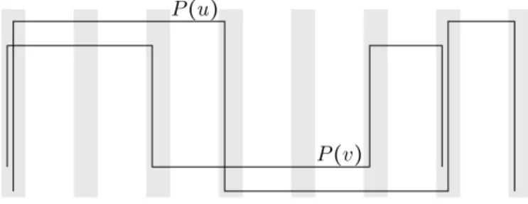
in at most k members of C. Reserve parallel segments of vertical grid-lines, one for each clique in C, such that all these segments see each other. We represent every vertex v by a path P(v) connecting the vertical segments corresponding to the k cliques containing v. The horizontal segments of P(v) are such that no horizontal segments of paths in the representation intersect. See Figure 4 for an illustration.
P(v) P(u)
Figure 4: A (2clℓ(G)−2)-bend representation: Each vertical gray part is reserved for a member
of C. Paths are inserted as demonstrated by P (u) and P (v) according to the cliques they are in.
Line graphs have local clique covering number at most 2, while the backwards direction does not hold, e.g., K5− e. Hence Theorem 3.4 generalizes a result of [4], stating that line graphs have bend-number at most 2.
Line graphs are claw-free and in [4] it was asked whether also claw-free graphs have bend-number at most 2. We feel that this is not the case.
Conjecture 2. There are claw-free graphs with arbitrary large bend-number.
4. Complete bipartite graphs
In this section we consider the bend-number of complete bipartite graphs. The interval-number of Km,n has been determined independently by Harary and Trotter [21] and Griggs and West [17], its track-number was determined by Gy´arf´as and West [19]. Both values are given by simple closed formulas, namely i(Km,n) = ⌈mn+1m+n⌉ and t(Km,n) = ⌈m+n−1mn ⌉. In contrast, a closed formula for the bend-number of complete bipartite graphs seems hard to obtain, as the results in this section illustrate.
It was shown by Biedl and Stern [4] that b(Km,n) ≤ 2m−2 for all n and that this bound is attained when n > 4m4−8m3+2m2+2m. Other than that the only
bound on b(Km,n) known before is b(Km,n) ≤ ⌈max{m,n}2 ⌉, due to Asinowski and Suk [3].
We present here two non-trivial lower bounds on b(Km,n): The Lower-Bound-Lemma I (Lemma 4.1) gives, depending on n, lower bounds on b(Km,n) ranging from m
2 to m − 1. It in particular implies that the construction of Asinowski and Suk [3] is tight in the case m = n, i.e., b(Km,m) = ⌈m2⌉. This es-pecially confirms a conjecture [4, 14] stating that for every k there is a graph G with b(G) = k. Moreover, we present in Theorem 4.4 a new construction assert-ing that the Lower-Bound-Lemma I is also tight at the other end of its range, i.e., b(Km,n) = m − 1 for all n roughly between m2 and m3/4. Interestingly, we obtain that the maximal n for which b(Km,n) ≤ k jumps from n ∈ θ(m2) to n∈ θ(m3) when going from k = m − 2 to k = m − 1.
Secondly, the Lower-Bound-Lemma II (Lemma 4.8) gives, depending on n, lower bounds on b(Km,n) ranging from m − 1 to 2m − 2. It improves the bound on the minimal n for which b(Km,n) = 2m − 2 to m4− 2m3+ 5m2− 4m + 1 (c.f. Theorem 4.9). With another construction in Theorem 4.5 we show that our new bound is nearly tight, i.e., we show that b(Km,n) ≤ 2m − 3 for n ≤ m4− 2m3+5
2m
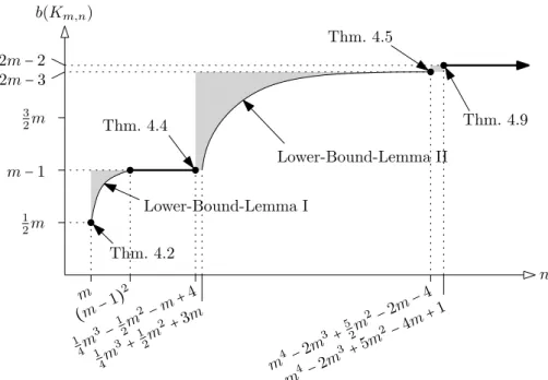
2− 2m − 4, which disproves a conjecture of Biedl and Stern [4], who suspected that this can be achieved only for n ∈O(m2). The Lower-Bound-Lemma II is almost tight at the lower, as well as at the upper end of its range. To summarize, we determine in this section b(Km,n) for several pairs of m,n and present two lower bounds for the general case. Our results are illustrated in Figure 5, where we sketch a region that contains the graph of b(Km,n) seen as a function of n for fixed m.
The bend-number of K2,n has been determined for all n in [3]: b(K2,n) = 2 iff n ≥ 5, b(K2,n) = 1 iff 2 ≤ n ≤ 4 and b(K2,n) = 0 iff n ≤ 1. Throughout this paper we denote the bipartition classes of Km,n by A ={a1, . . . , am} and B={b1, . . . , bn} and will always assume 3 ≤ m ≤ n.
We start with the first lower bound on the bend-number of Km,n. In the lemma below, as well as in the second lower bound in Lemma 4.8, we present an inequality with variables m, n and k that is valid for every k-bend representation of Km,n. Fixing m and n, we obtain a lower bound on k = b(Km,n); Fixing m and k we obtain an upper bound on the maximum n such that b(Km,n) ≤ k. Lemma 4.1 (Lower-Bound-Lemma I). For every k-bend representation of Km,n we have
(k + 1)(m + n) ≥ mn +√2k(m + n).
Proof. Fix a k-bend representation of Km,nand assume w.lo.g. that every path has exactly k bends. LetL be the set of all grid-lines that support any segment of any path. Further, letG be the set of grid-points that support a bend of any path in the representation, andG3⊆G be those grid-points that support at least 3 bends.
Now, look at the rightmost or topmost grid-edge of each of the k+1 segments of every path P(v). If this grid-edge is shared by another path P(w) (there can be only one, because the graph is bipartite), we assign v to the edge{v,w} in the graph. This way
b(Km,n) n 1 2m m− 1 3 2m 2m − 3 2m − 2 m (m− 1) 2 1 4m 3 − 1 2m 2 − m+ 4 1 4m 3 + 1 2m 2 + 3m m4 − 2 m3 + 5 2m 2 − 2m − 4 m4 − 2 m3 + 5 m2 − 4 m +1 Thm. 4.4 Thm. 4.5 Thm. 4.2 Lower-Bound-Lemma I Lower-Bound-Lemma II Thm. 4.9
Figure 5: Illustration of the lower and upper bounds on b(Km,n) presented in this section.
The gray region contains the graph of the function n ↦ b(Km,n) for fixed m. Filled circles
and solid lines correspond to exact values.
every vertex is assigned to at most k + 1 edges, every edge is assigned at least once,
at the rightmost (topmost) grid-edge of every line in L either no
assign-ment is done or an edge is assigned twice, and
at the left and bottom grid-edge of every point inG3either no assignment
is done or an edge is assigned twice.
Hence we have(k + 1)∣V (Km,n)∣ ≥ ∣E(Km,n)∣ + ∣L∣ + 2∣G3∣, i.e.,
(k + 1)(m + n) ≥ mn + ∣L∣ + 2∣G3∣. (1) Since every path has exactly k bends and every grid-point supports at most 4 of them, we get∣G∣ ≥ k(m+n)−4∣G3∣
2 +∣G3∣ = k(m+n)
2 −∣G3∣. Now if we have ℓhhorizontal and ℓv vertical lines inL, and these lines cross in at least ∣G∣ grid-points, then ∣L∣ = ℓh+ ℓv with ℓh⋅ ℓv≥∣G∣. The sum is minimized by ℓh= ℓv=
√
∣G∣. Hence, ∣L∣ ≥ 2√∣G∣ ≥√2k(m + n) − 4∣G3∣ ≥
√
2k(m + n) − 2√∣G3∣. (2) Putting (1) and (2) together we obtain
(k + 1)(m + n) ≥ mn +√2k(m + n) − 2√∣G3∣ + 2∣G3∣ ≥ mn + √
2k(m + n), which completes the proof.
The Lower-Bound-Lemma I is meaningful only for k ≤ m − 2. Indeed if k ≥ m − 1, then the inequality in the Lower-Bound-Lemma I is valid for all n. The reason is that for k ≥ m − 1 the paths for B could have each edge-intersection on a different segment. However, the Lower-Bound-Lemma I gives non-trivial lower bounds on b(Km,n) ranging from m
2 to m − 1 depending on n. These bounds turn out to be best-possible at both ends of this range, i.e., we can determine b(Km,n) exactly for some particular pairs of m and n (c.f. Theorem 4.2 and Theorem 4.4).
Theorem 4.2. For all m ≥ 3 we have b(Km,m) = ⌈m2⌉.
Proof. As mentioned above in [3] it is shown that b(Km,n) ≤ ⌈max(m,n)/2⌉. For equality we will prove that Km,mcannot be represented with less than⌈m
2⌉ bends. We use the Lower-Bound-Lemma I with m = n and k = m−12 ≥⌈m
2⌉ − 1. Bringing everything on the left-hand-side we obtain
(m −√2m(m − 1))/2m ≥ 0, which is a contradiction for m ≥ 3.
With Theorem 4.2 we can confirm a conjecture of [14].
Corollary 4.3. For every k ≥ 0 there is a graph G with b(G) = k.
From the Lower-Bound-Lemma I we get that the bend-number of Km,nis at least m−1 if n ≥(m−1)2. Next we show that this bound is tight, that is, we can find a(m − 1)-bend representation of Km,neven for n ≈m3
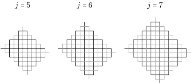
4 (c.f. Theorem 4.4). Our construction (as well as the one in Theorem 4.5) is based on the fact that two(2j −1)-bend paths can cross in ℓ(ℓ+1) points as indicated in Figure 6. In Lemma 4.7 we will show that this is best-possible. Formally, P1 may be described as starting at(0,0) with a horizontal segment to the right, followed by a downwards segment, and then alternate left and right and up and down. The length of the i-th horizontal segment is 2j + 3 − 2i and of the i-th vertical segment is 2i. The path P2 is obtained by rotating P1 by 180 degrees and translating the starting point to(2j +2,−1). We call the pair (P1, P2) a pretzel.
j= 5 j= 6 j= 7
For the next two constructions we “blow up” the pretzels in Figure 6: We split the vertices in A evenly into A1=(a1
1, . . . , a1⌊m
2⌋) and A2=(a
2
1, . . . , a2⌈m 2⌉).
Then, for fixed j we construct a set of m(2j−1)-bend paths such that every path representing a vertex from Ai looks like Pi just with changed segment-lengths (i = 1, 2). More precisely, P(a11) has starting point (1,1), its i-th horizontal segment is of length⌊m
2⌋(m − i) + ⌈ m
2⌉(m − i + 1) and its i-th vertical segment is of length⌊m 2⌋(i − 1) + ⌈ m 2⌉(i + 1). For h = 2,... ,⌊ m 2⌋, P(a 1
h) has starting point (h,h), its i-th horizontal segment is 2 units shorter than the i-th horizontal segment of P(a1h−1) and its i-th vertical segment is 2 units longer than the i-th vertical segment of P(a1h−1). In the end, we enlarge all starting segments such that P(a1h) has starting point (1,h) (h = 1,... ,⌊m
2⌋) and all ending segments such that all endpoints lie on one line.
The paths representing A2arise from P2 in an analogous way by interchang-ing floor and ceilinterchang-ing functions in the length formulas. Their startinterchang-ing points are at (⌊m2⌋(m − 1) + ⌈m2⌉m + 1,1 − h) (h = 1,...,⌈m2⌉). The blown-up pretzel for m= 6 and j = 3 is depicted in Figure 7.
Crossings in a blown-up pretzel are either formed by paths from the same Ai (type 1i) or from A1 and A2 (type 2). Type 1i crossings form blocks of size ∣Ai∣×∣Ai∣ and the type 2 crossings come in blocks of size ∣A1∣×∣A2∣. Some blocks of type 1iare located around one bend of the corresponding paths. These blocks have triangular instead of quadrangular shape. All blocks form a checkerboard pattern. In Figure 7 the type 2 blocks are highlighted by gray boxes.
We group the blocks in a blown-up pretzel into four quadrants as illustrated in Figure 7. I.e., we choose a horizontal and a vertical line that separate the horizontal and vertical ends of paths for A1 from those for A2, respectively. Theorem 4.4. If m is even, then b(Km,1/4m3−1/2m2−m+4) = m − 1. If m is odd, then b(Km,1/4m3−m2+3/4m) = m − 1.
Proof. We represent the bipartition class A by a blown up pretzel, where j ∶=
⌊m
2⌋. That is, if m is odd we use one bend less than allowed. We analyze the blocks of the blown-up pretzel. Inside a quadrant, the order in which the paths P(aih) (h = 1,... ,⌈m2⌉, i = 1,2) appear horizontally and vertically in the blocks is always the same. See Figure 8 for an example.
Next we explain how to represent a subset of vertices of B as small staircases with m − 1 bends inside the first (that is the top-right) quadrant. Pick a block of type 2 inside the quadrant. We use staircases that go from lower left to upper right. Half of the paths start with a horizontal segment and the other half with a vertical segment. All segments have length 1. As illustrated in Figure 8, it is possible to put m paths into one block of type 2. If m is even, two paths lie completely within the blocks, m−22 paths have segments lying in a triangular sector in the type 1i blocks above and to the left, and m−22 paths have segments in a triangular sector in the type 1iblocks below and to the right. If m is odd, it is one path that lies completely within the blocks, m−1
2 paths have segments in a triangular sector in the type 1iblocks above and to the left, and m−12 paths have segments in a triangular sector in the type 1i blocks below
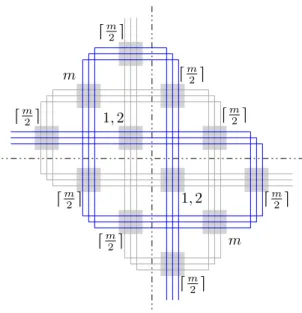
⌈m 2⌉ ⌈m 2⌉ ⌈m 2⌉ ⌈m 2⌉ ⌈m 2⌉ ⌈m 2⌉ ⌈m 2⌉ ⌈m 2⌉ 1, 2 1, 2 m m
Figure 7: A blown up pretzel for m = 6 and j = 3. The dashed lines indicate the four quadrants used in the proof of Theorem 4.4. Type 2 blocks are highlighted by gray boxes. Next to the boxes the numbers of staircases that can be introduced there are noted. For better readability grid-edges between distinct blocks are drawn longer.
and to the right. Note that the type 1i blocks above and to the right may be triangular, i.e., correspond to a set of bends and that in this case still every segment establishes an edge-intersection. This case is depicted in Figure 8.
The staircases for each type 2 block are completely contained in a square area as illustrated in Figure 8. Since squares for distinct blocks are disjoint, no two staircases have an edge-intersection. Finally, we remove all staircases that are crossing the coordinate axes, i.e., keep only those completely contained in the first quadrant.
Next we extend the above construction to all four quadrants by mirroring the staircase paths along the coordinate axes. Since type 2 blocks correspond to crossings between P1 and P2in the underlying pretzel, there are ⌊m2⌋(⌊m2⌋ + 1) of them. Note further that at type 2 blocks close to the coordinate axes we have removed some staircases that crossed the coordinate axes. In particular we have introduced only ⌈m2⌉ staircases at a type 2 block close to one coordinate axis. There are 2(2j − 1) = 4⌊m2⌋ − 2 of these blocks. At the two type 2 blocks next to two coordinate axes all but 1, respectively 2, paths have been removed for m odd, respectively m even. In Figure 7 we summarize the number of staircases introduced at each type 2 block for m = 6 and j =⌊m
2⌋ = 3. In total for odd m we obtain(⌊m
2⌋(⌊ m 2⌋ + 1) − (4⌊ m 2⌋))m + (4⌊ m 2⌋ − 2)⌈ m 2⌉ + 2 staircases, which simplifies to 1
4m
3− m2+ 3
4m. For even m we get the same formula plus 2, which simplifies to 1
4m 3− 1
2m
2− m + 4. Hence we have con-structed a(m − 1)-bend representation of Km,1/4m3−1/2m2−m+4 for m even and
P(a11) P(a11) P(a11) P(a11) P(a11) P(a12) P(a12) P(a13) P(a13) P(a14) P(a14) P(a14) P(a14) P(a14) P(a21) P(a21) P(a21) P(a21) P(a21) P(a22) P(a22) P(a22) P(a22) P(a23) P(a23) P(a23) P(a23) P(a24) P(a24) P(a24) P(a24) P(a24) ⋯ ⋯ ⋯ ⋯
Figure 8: Inserting m staircases for each type 2 block in the first quadrant. For better readability grid-edges between distinct blocks are drawn longer.
Km,1/4m3−m2+3/4m for m odd, which completes the proof.
Remark. By a straight-forward application of the Lower-Bound-Lemma I one sees that already for much smaller n than in the above theorem m − 1 bends are necessary, i.e., b(Km,(m−1)2) ≥ m − 1 for all m ≥ 3.
It is known that the bend-number of Km,n can be as large as 2m − 2 [3], but not larger [14]. Let n∗ denote the maximal n for which b(Km,n) < 2m − 2. Asinowski and Suk [3] proved that n∗ ∈ O(mm). This was later improved by Biedl and Stern [4] to n∗ ≤ 4m4− 8m3+ 2m2+ 2m, who also conjectured that n∗ ∈ O(m2). Note that Theorem 4.4 above implies that n∗ ≥ 1
4m
3− m2, and hence disproves this conjecture.
Next we show that n∗≥ m4−2m3+5 2m
2−2m−4, i.e., we find a(2m−3)-bend representation of b(Km,n) with n = m4− 2m3+52m
2− 2m − 4, see Theorem 4.5. Afterwards, we present the Lower-Bound-Lemma II, a special case of which improves the upper bound on n∗ to m4− 2m3+ 5m2− 4m, see Theorem 4.9. Hence we have narrowed n∗ down to an interval of length less than 2.5m2. Theorem 4.5. If n ≤ m4− 2m3+5
2m
2− 2m − 4 then b(K
m,n) ≤ 2m − 3.
Proof. Again, we use blown-up pretzels. This time, we set j ∶= m−1, i.e., we use
(2m−3)-bend paths. We scale the blown-up pretzel by a factor of 2m2+ 3, such that between any two horizontal (vertical) segments we have 2m2+ 2 horizontal (vertical) grid-lines.
We start by defining a single-bend path, that is a 1-bend path, P(b) for every vertex in b ∈ B. Every P(b) has an edge-intersection with two paths for A. In a second step every P(b) will be extended to a (2m − 3)-bend path that has an edge-intersection with P(a) for every a ∈ A. Let us consider the first, that is the top-right, quadrant only. The paths for the q-th quadrant are defined analogously by rotating the entire representation by(q−1)π2 in counterclockwise direction, q = 1, 2, 3, 4.
We number the vertical segments of paths for A that intersect the first quadrant by v1, v2, v3, . . .according to their left-to-right order, i.e., by increasing x-coordinate. Similarly, we number the horizontal segments that intersect the first quadrant by h1, h2, h3, . . . according to their top-down order, that is by decreasing y-coordinate. Consider a crossing vi∩ hk between two segments corresponding to two distinct paths. We define two single-bend paths that both have a bend at the crossing point p. The corresponding vertical segments have length 2i and lie on different sides of p. The two corresponding horizontal segments have length max(1,2(⌈m
2⌉ − k)) and lie on different sides of p, too. In particular, the horizontal segments have length more than 1 only if k <⌈m
2⌉. See Figure 9 for an example.
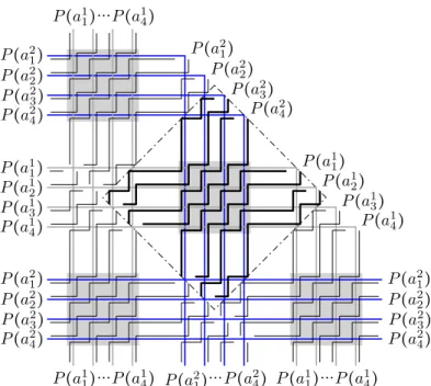
P(a11) P(a11) P(a11) P(a12) P(a12) P(a12) P(a21) P(a21) P(a21) P(a22) P(a22) P(a22)
Figure 9: Interlacing two single-bend paths for every crossing and one single-bend path at each but the left-most bend. In a second step these paths are extended by snake paths in the direction indicated by the arrows.
We introduce another set of single-bend paths for each but the left-most bend in the first quadrant. Let the bend be the top-end of the vertical segment vi. We define a single-bend path edge-intersecting vi and the horizontal segments hk that has a bend with vi−1. The horizontal and vertical segment of the
single-bend path has length 2m2+ 3 + max(1,⌈m
2⌉−k) and 2m
2+ 3 + 2i, respectively. In particular, each vertical intersection has length 2i and a horizontal edge-intersection has length more than 1 only if k <⌈m
2⌉. See Figure 9 for an example. Next we extend every single-bend path P at its vertical end. Let ℓ(P) be the horizontal grid-line through the vertical end of P . From the initial scaling follows that there is at least one further horizontal grid-line between every two ℓ(P), as well as between every ℓ(P) and every horizontal segment of the blown-up pretzel. Now, for every vertex a ∈ A, except for the two whose paths are already edge-intersecting P , consider the rightmost vertical segment of P(a) in the fourth, that is the top-left, quadrant that crosses ℓ(P). We extend P by a snake path connecting all these segments, i.e, every new vertical segment of P is contained in a segment of some P(a), has length 1 and its lower end lies on ℓ(P). In Figure 9 the first segment of each snake is indicated by an arrow pointing to the left.
For some 1-bend paths P not all paths for A cross the horizontal line ℓ(P). However, this is the case only if P has an edge-intersection with hk for k <⌈m
2⌉. We let the snake extension for these paths edge-intersect only those paths P(a) that indeed cross ℓ(P). In order to establish the remaining edge-intersections we extend the 1-bend path P at its left-end, too. More precisely, let ℓ′(P) be the vertical grid-line through the left-end of P . For each path P(a) that has no edge-intersection with P yet, consider the topmost horizontal segment of P(a) within the first quadrant. We extend P by a snake path of which every new horizontal segment is contained in such a topmost segment, has length 1 and whose left end lies on ℓ′(P).
We claim that we have defined a(2m −3)-bend representation of Km,nwith n= m4− 2m3+5
2m
2− 2m − 4. It is easy to check that every path P(b) for a vertex b in B has 2m − 3 bends and edge-intersects all paths for A. Consider one quadrant Q, say the first. We consider all horizontal edge-intersections in Q: Most of the single-bend paths that have been introduced within Q have a horizontal edge-intersection that has length 1 and lies next to a vertical segment of some path for A. There exist horizontal edge-intersections that are longer, but only within the top-most ⌈m
2⌉ horizontal segments. Secondly, there are horizontal edge-intersections in Q corresponding to snake extensions of single-bend paths in the second quadrant. Those edge-intersections consist of only one grid-edge that does not lie next to a vertical segment of some path for A. Moreover, these edge-intersection are contained in the bottommost horizontal segments in Q of each P(a), i.e., each is contained in some hk for k > ⌈m2⌉. Finally, there are some edge-intersections corresponding to snake extensions of single-bend paths in Q. These edge-intersections consist of only one grid-edge that does not lie next to a vertical segment of some path for A, and are chosen to be top-most, i.e., each is contained some hk for k ≤⌈m
2⌉.
It follows that no two paths for B have a horizontal edge-intersection in the first quadrant. An analogous reasoning holds for vertical edge-intersections, as well as for the other quadrants.
paths P1, P2 in the underlying pretzel have(j2) self-crossings each, while there are j(j + 1) crossings between P1 and P2. Moreover, in the blown-up pretzel at every bend of one Pi each pair of paths crosses (i = 1, 2). Thus, two paths for vertices in the same Ai cross 2(j2) + 2j − 1 = j(j + 1) − 1 times, and two paths, one for a vertex in A1 and the other for a vertex in A2, cross j(j + 1) times. In terms of m, every pair of paths for the same Ai crosses m(m − 1) − 1 times, and every pair of paths for distinct Ai crosses m(m − 1) times. Hence the total number of crossings between paths representing vertices in A is given by⌊m2⌋⌈m2⌉m(m − 1) + ((⌈m/2⌉2 ) + (⌊m/2⌋2 ))(m(m − 1) − 1).
We have introduced two paths for every crossing in the blown-up pretzel and one path for all but one bend in each quadrant. Thus we have constructed a (2m − 3)-bend representation of Km,nwith n = 2⌊m2⌋⌈m2⌉m(m − 1) + 2((⌈m/2⌉2 ) + (⌊m/2⌋
2 ))(m(m − 1) − 1) + m(2m − 3) − 4 = ⌊m
4− 2m3+5 2m
2− 2m − 4⌋.
Next we present a second lower bound on b(Km,n) that is weaker than the Lower-Bound-Lemma I for n < m2, but stronger for n > m3.
Lemma 4.6. In a k-bend representation of Km,n let c denote the total number of crossings between the paths P(a1),... ,P(am). Then we have:
n(2m − k − 2) ≤ 2c + 2(k + 1)m
Proof. Fix a k-bend representation of Km,n. We associate every path P(b), b∈ B, with some crossings between paths for A and some endpoints of segments of paths for A. Every crossing will be associated with at most two paths for B, and every endpoint of a segment with at most one path for B.
Consider a vertex b ∈ B and its path P(b). Let l be the number of segments of P(b) on which no edge-intersection occurs. Going along P(b) we obtain a total order for the edge-intersections P(b) ∩ P(a) for all a ∈ A. For two edge-intersections P(b)∩P(a) and P(b)∩P(a′) that appear consecutive in this order let s and s′ be the corresponding segments, respectively.
If s and s′lie on the same segment of P(b), then we associate with P(b) the two endpoints of s and s′with no edge-intersection between them. Since b has degree m, m edge-intersections occur on k + 1 − l segments of P(b). Thus we associate with P(b) in this first step at least 2(m−(k+1−l)) = 2m−2(k+1)+2l endpoints of segments of paths for A.
Now assume that s and s′ lie on two consecutive segments of P(b). If s and s′cross at the corresponding bend of P(b), we associate this crossing with P(b). Otherwise at least one endpoint of s or s′ lies on P(b) and has no edge-intersection between itself and the bend of P(b). We associate P(b) with this endpoint. Since P(b) has edge-intersections on k + 1 − l of its k + 1 segments we associate with P(b) in this second step at least k − 2l crossings between paths for A or endpoints of segments of paths for A.
Note that every endpoint of a segment of a path for A is associated with at most one P(b) and every crossing between paths for A is associated with at most two paths for B. Hence in total we have associated with all the paths for B at least n(2m − 2(k + 1) + 2l + k − 2l) = n(2m − k − 2) crossings and endpoints
of paths for A. On the other hand every P(a) with a ∈ A has only 2(k + 1) endpoints of segments and the total number of crossings between paths for A is c. Thus n(2m − k − 2) ≤ 2c + 2(k + 1)m, which completes the proof.
We want to use the inequality in Lemma 4.6 as a lower bound on k for fixed m and n. Therefore it remains to prove an upper bound on c, that is on the number of times m k-bend paths can cross each other. We content ourselves with bounding the number of times two k-bend paths can cross in case k is odd. Lemma 4.7. Two(2j − 1)-bend paths cross in at most j(j + 1) points.
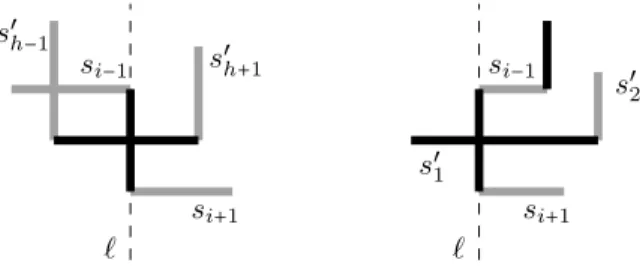
Proof. Consider two given (2j − 1)-bend paths P and P′. Both have exactly j horizontal and j vertical segments. We color the vertical segments of P and the horizontal segments of P′blue and the remaining segments red. Now every crossing is monochromatic. We partition the pairs of segments that have the same color but come from different paths into four sets. SetB contains all blue pairs that do cross andB all blue pairs that do not cross. Similarly R and R are defined for red segments. Along each path we index the segments, starting with its blue end, i.e., s1 and s′1 are blue and P =(s1, . . . , s2j) and P′=(s′1, . . . , s′2j). Consider a blue crossing{si, s′h} ∈ B and the grid-line ℓ containing si. Each of si−1, si+1, s′h−1, s′h+1, if it exists, is red and lies completely on one side of ℓ. Moreover s′h−1 and s′h+1 cannot lie on the same side since s′h crosses ℓ. Now consider si−1 (or si+1) and the segment of P′ on the other side of ℓ. This pair evidently is inR. This way we associate up to two red non-crossings with every blue crossing, even if there are more (see Figure 10).
s′1 s′2 s′h−1 s′h+1 si−1 si−1 si+1 si+1 ℓ ℓ
Figure 10: A blue crossing is associated with every pair of red segments from different sides of ℓ: The blue crossing on the left is associated with {si−1, s′h+1} and {si+1, s′h−1}. The blue
crossing on the right is associated with no red non-crossing.
Next we partitionB in two ways. First, divide B into B0,B1, andB2 accord-ing to the number of red non-crossaccord-ings, the blue crossaccord-ings are associated with in the above way. Second, we writeB(s1) for the set of blue crossings s1 partic-ipates in and do the same with s′1. Furthermore, we denoteBi(s′1) ∶= Bi∩B(s′1) for i = 0, 1, 2. If a blue crossing is associated with no red non-crossing, then s′
1 has to participate in the crossing, i.e., B0=B0(s′1). Moreover, a blue crossing is associated with exactly one red non-crossing if either s′
1 is involved and we associate exactly one non-crossing or s1 is involved in the crossing but not s′
This is, B1 =(B(s1)/B(s′1)) ∪ B1(s′1). Note that every red non-crossing is as-sociated with at most two blue crossings and hence we have∣B1∣ + 2∣B2∣ ≤ 2∣R∣. This leads to:
2∣B∣ ≤ 2∣R∣ + ∣B(s1)/B(s′1)∣ + ∣B1(s′1)∣ + 2∣B0(s′1)∣
First, note that Since P, P′ have only j blue segments we clearly have ∣B(s1)/B(s′1)∣ ≤ j − 1.
Second, observe the following: On the path P between any two blue seg-ments contributing to aB0(s′1)-crossing, either there is another blue segment contributing to B0(s′1) or there is a blue segment of P that participates in a B2(s′1)-crossing or there is one which does not cross s′1 at all. Hence, because P has only j blue segments, we have 2∣B0(s′1)∣ − 1 + ∣B1(s′1)∣ ≤ j.
Plugging both into the above inequality, we calculate 2∣B∣ ≤ 2∣R∣+2m. Thus, ∣B∣ − ∣R∣ ≤ j. Now adding j2 on both sides we obtain: ∣B∣ + ∣R∣ ≤ j2+ j, where R denotes the set of red crossings. In particular, the number of crossings is at most j(j + 1).
Note that pretzels, see Figure 6, witness that the bound in the above lemma is tight. The following question arises:
Question 2. What is the maximum number of crossings that two 2j-bend paths can have?
Next we combine Lemma 4.6 and Lemma 4.7 to achieve a second Lower-Bound-Lemma.
Lemma 4.8 (Lower-Bound-Lemma II). For every k-bend representation of Km,n we have
n(2m − k − 2) ≤ m(m − 1)⌈k+ 1 2 ⌉⌈
k+ 3
2 ⌉ + 2(k + 1)m.
Proof. By Lemma 4.7 two k-bend paths can cross in at most⌈k+12 ⌉⌈k+32 ⌉ points.
(If k is even we simply take the bound for two(k + 1)-bend paths.) Hence m k-bend paths cross in at most(m2)⌈k+12 ⌉⌈k+32 ⌉ points. Plugging this into Lemma 4.6 gives the claimed inequality.
We think that the bound on the number of crossings between m k-bend paths can be further improved. In particular we conjecture that for odd k no three k-bend paths can pairwise cross in k+12 k+32 points. This would imply that for odd k the blown-up pretzel maximizes the total number of crossings between m k-bend paths.
Theorem 4.9. If n > m4− 2m3+ 5m2− 4m, then b(K
m,n) = 2m − 2. Note that
this leaves only a quadratic discrepancy to the bound in Theorem 4.5.
Proof. If m = 1, then Km,nis a star and thus an interval graph, i.e., b(K1,n) = 0 for all n > 0.
For m > 1 assume that b(Km,n) ≤ 2m − 3. Then by the Lower-Bound-Lemma II with k = 2m − 3 we get n ≤ 2(m2)(m − 1)m + 2(2m − 2)m = m4− 2m3+ 5m2− 4m.
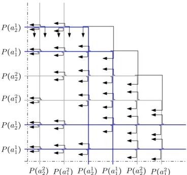
On the other hand it is known [14] that b(Km,n) ≤ 2m − 2, regardless of n, as illustrated in Figure 11.
Figure 11: A representation verifying b(Km,n) ≤ 2m − 2.
Applying all the above machinery together with the 2-bend representation of K3,10 in Figure 1 we obtain that b(K3,n) is 1 if n ≤ 2, 2 if 3 ≤ n ≤ 10, 3 if 11 ≤ n ≤ 39 and 4 if n ≥ 61. The first unknown case is 3 ≤ b(K3,40) ≤ 4.
5. Degeneracy
In [4] an acyclic orientation of G with maximum indegree k is referred to as a k-regular acyclic orientation. The degeneracy dgn(G) of G is the smallest number k, such that G has a k-regular acyclic orientation, see [27]. In this section we provide a tight upper bound on the bend-number of graphs with a fixed degeneracy. In [4] the following result was suspected to be true.
Theorem 5.1. Every graph G has a(2dgn(G) − 1)-bend representation.
Proof. Take a dgn(G)-regular acyclic orientation of G in the above sense. A
topological ordering then gives us a building recipe for G, where every new vertex will be connected to at most dgn(G) vertices of the already constructed part. We construct a(2dgn(G) − 1)-bend representation simultaneously to the building process of G. We maintain the following invariant for the(2dgn(G) − 1)-bend representation of the already constructed subgraph G′ of G: For every vertex v∈ V(G′) the path P(v) contains a vertical subsegment s(v) and a horizontal subsegment ¯s(v) both displaying v. Moreover all the vertical subsegments s(v) for v ∈ V(G′) see each other. In the first step, when G′is just a single vertex v, this invariant holds by taking any 1-bend path for v.
Now when the next vertex v is added to G′, consider the k neighbors of v in G′. In particular k ≤ dgn(G). Let these neighbors be labeled v1, . . . , vk. We define the grid path P(v) for v as follows: We start with P(v) being any grid path connecting s(v1),... ,s(vk−1) and extend the last vertical segment of P(v) by one grid-edge, so that its end-point has a different y-coordinate than its bends. (If k = 1, we define P(v) to be a single grid-point on a grid-line that
intersects all the s(vi).) Next, we extend P(v) at its end-point by three further segments so that the last horizontal segment is completely contained in ¯s(vk). We refer to Figure 12 for an example of this construction. (If k = 0, we define P to be any 1-bend path whose vertical segment sees all the s(vi).)
s(v) ¯ s(v) s(v1) s(v2) s(v3) s(v4) ¯ s(v4)
Figure 12: Building a (2dgn(G) − 1)-bend representation of G, a path P (v) is inserted. Vertex-displaying subsegments before and after the insertion are highlighted with light-gray and dark-gray, respectively.
The path P(v) has 2k − 2 + 3 ≤ 2dgn(G) − 1 bends and is edge-intersecting exactly the paths corresponding to v1, . . . , vk. Moreover, the last vertical seg-ment s of P(v) displays v and sees all previous vertical subsegments. Thus for each vertex w in G′∪ v we can find a vertical subsegment s(w) as required in our invariant. Finally, a horizontal subsegment for vk and v can be chosen as a subset of the previous ¯s(vk) and any horizontal segment of P(v), respectively. Thus our invariant is maintained for the new subgraph G′∪ v, which proves the theorem.
Next, we show that Theorem 5.1 is worst-case optimal, even for bipartite graphs.
Theorem 5.2. For every positive integer m there is a bipartite G with dgn(G) = mand b(G) ≥ 2dgn(G) − 1.
Proof. The graph G arises from a Km,nwith large enough n =∣B∣, which will be determined later. First, for every m-subset B′of B we add m(2m − 2) + 1 new vertices, each having B′as its neighborhood. The set of the(m(2m−2)+1)(mn) added vertices is denoted by C. Moreover, for every m-subset C′of C we add m(2m − 2) + 1 new vertices, each having C′ as its neighborhood. This set of vertices is denoted by D.
Clearly, dgn(G) = m. Now suppose b(G) ≤ 2m − 2 and consider the Km,n induced by A and B. Indeed by Lemma 4.7 there are at most(m2)m(m + 1) crossings between the m(2m−2)-bend paths for A. Every crossing can lie on at most two paths for B. Moreover, the paths for A have only m(4m−4) endpoints and every such endpoint lies on at most one path for B. It follows that for at least n − 4m4 vertices b ∈ B the m edge-intersections of P(b) with paths for A
appear on exactly every second segment of P(b). By this with increasing n the paths for an arbitrarily large subset ̃B⊂ B must look like in Figure 11, i.e., all edge-intersections of paths for ̃B with paths for C have the same orientation, say vertical. Additionally, there are many pairs B1, B2 of m-subsets of ̃B with the property that every path for B1 lies to the left of every path for B2.
We fix m distinct m-subsets B1, . . . , Bm of ̃B, such that every path for B1 lies to the left of every path for B2∪ . . . ∪ Bm. Hence the path for every vertex c∈ C whose neighborhood is B1 lies completely to the left of every path for a vertex in C whose neighborhood is one of B2, . . . , Bm.
P(c1) P(c2) P(c3)
Figure 13: A part of a hypothetical (2dgn(G) − 2)-bend representation of G. The paths for the sets ̃Band ̃C= {c1, c2, c3} are depicted gray and thick, respectively.
Now for every Bithere are m(2m−2)+1 vertices in C whose neighborhood is Bi, that is, one more than there are bends in the paths for Bi. Since every bend of a path for Bi lies on at most one path for C, there is for every i ∈{1,...,m} at least one vertex ci∈ C whose neighborhood is Bi and for which the vertical segments of P(ci) are completely contained in segments of path for Bi (see Figure 13 for an example). In G there is a set D′⊂ D of m(2m − 2) + 1 vertices with neighborhood C′∶={c1, . . . , cm}; again one more than there are bends in C′. Hence of at least one path for a vertex in D′ all horizontal segments are contained in segments of paths for C′. But this is impossible since the path P(c1) lies to the left of the paths for all other vertices in C′.
In [4] a (not necessarily acyclic) orientation of G with maximum indegree k is referred to as a k-regular orientation. The pseudo-arboricity pa(G) of G is the smallest number k, such that G has a k-regular orientation, see [30]. In [4] it is shown that b(G) ≤ 2pa(G) + 1 and b(G) ≤ 2pa(G) for bipartite G. The (bipartite) graph in Theorem 5.2 has pseudo-arboricty m, which can be seen using pa(G) = maxS⊆V (G)⌈∣E[S]∣∣S∣ ⌉, see [11]. Therefore, we have b(G) ≥ 2pa(G) − 1.
Question 3. What is the maximal bend-number of graphs with bounded pseu-do-arboricity?
6. Treewidth
A k-tree is a graph that can be constructed starting with a(k+1)-clique and in every step attaching a new vertex to a k-clique of the already constructed
graph [28]. The treewidth tw(G) of a graph G is the minimum k such that G is a subgraph of some k-tree [32].
In [14] Golumbic, Lipshteyn, and Stern show, that every graph G with tw(G) ≤ 1, i.e., every forest, has b(G) ≤ 1. In [22] it is shown that graphs of treewidth at most 2 have bend-number at most 2. In this section we present a tight bound for the maximum bend-number of graphs of bounded treewidth. To judge the upper bounds of the bend-number in terms of the bounded treewidth, we remark, that there is a graph G with tw(G) = 1 = b(G), i.e. the bound for the class of graphs of treewidth 1 is tight. The general lower bound is a simple corollary of a previously mentioned theorem.
Corollary 6.1. For every k ≥ 2 there is a graph G with tw(G) = k and b(G) = 2⋅ tw(G) − 2.
Proof. Theorem 4.9 states, that the complete graph Km,n with n ≫ m has bend-number 2m− 2. Clearly this graph has treewidth m.
Theorem 6.2. Let k ≥ 2. For every graph G with tw(G) ≤ k we have b(G) ≤ 2k− 2.
Proof. The cases tw(G) ≤ 1,2 are solved by [14, 22]. So let tw(G) = k ≥ 3. Let
˜
Gbe a k-tree that is a super-graph of G. Then ˜Gcan be iteratively constructed starting with a k-clique and adding one-by-one the remaining vertices to the graph, such that the neighbors of each vertex in the already constructed graph form a k-clique in ˜G. Similarly to the proof of Theorem 5.1 we construct a (2k − 2)-bend representation of G along this building sequence of G. Again when a new vertex v is added to the already constructed subgraph G′ of G, then v has at most k neighbors in G′. But this time only few k-sets of vertices can form the neighborhood of a later added vertex and we know exactly which – namely the k-cliques in ˜G.
We maintain an invariant on the(2k − 2)-bend representation of the graph G′. Loosely speaking, we ensure that for “almost every” vertex w we have a vertical and a horizontal subsegment that displays w and crosses the x-axis and y-axis, respectively. In particular all these vertical subsegments, as well as all the horizontal ones, see each other. More formally, we fix a coordinate cross with origin o, horizontal x-axis and vertical y-axis. We say that a vertex w is
displayed horizontally (vertically) if there is a horizontal (vertical) subsegment
of P(v) that displays v and intersects the y-axis (x-axis) in an interior point. We require that for every k-set W of vertices in G′ that forms a k-clique in ˜G one of the following invariants holds.
Invariant A: There exists a vertex w1 ∈ W such that every w ∈ W ∖ w1 is displayed horizontally, and every w ∈ W is displayed vertically. Moreover, on either side of o there is at least one of the vertical subsegments. This invariant is also satisfied if it holds exchanging horizontal and vertical. It is illustrated in Figure 14.
Invariant B: There exist two adjacent vertices w1, w2 ∈ W such that every w∈ W ∖ w1 is displayed horizontally, and every w ∈ W ∖ w2 is displayed vertically. Moreover, on the same grid-line as the subsegment for w1 lies a subsegment s(w1w2) that displays the edge (w1, w2). This invariant is also satisfied if it holds exchanging horizontal and vertical. It is illustrated in Figure 15. w1 w1 w1 w2 w2 w2 w2 w2 w2 w3 w3 w3 w3 w3 w3 P(v) P(v) P(v)
Figure 14: Invariant A for a k-clique {w1, w2, w3} of ˜Gand how to insert the new path P (v)
(drawn bold). Left: v is adjacent to every vertex in the k-clique. Middle: v not adjacent to at least one vertex in the k-clique. Right: v is adjacent only to the unique vertex with a vertical subsegment to the right of o.
When the next vertex v is added to G′ in the building sequence of G we define the corresponding grid path P(v) as follows. Let W be the k-clique of ˜G that contains the neighborhood of v in G′. First suppose that invariant A holds for W . We assume w.l.o.g. that every w ∈ W is displayed vertically and every w∈ W∖ w1 is displayed horizontally. Let S be the set of vertical subsegments that correspond to the neighbors of v in G′, display the corresponding vertex, and intersect the x-axis. We define P(v) to be a grid path that connects S and lies completely on one side of the x-axis. If ∣S∣ = k, i.e., v is adjacent to every vertex in W , then P(v) is a (2k − 2)-bend path. If ∣S∣ ≤ k − 1, we extend P(v) by two segments, such that either segment intersects a coordinate axis. If the vertical subsegments of all but one vertex w∗∈ W lie on the same side of o and v is adjacent only to w∗, i.e.,∣S∣ = 1, then we extend P(v) by two further segments that intersect the coordinate axes. In particular P(v) is extended by four segments in total. This case is exemplified in the right of Figure 14. (Here we make implicit use of the assumption k ≥ 3 to ensure that P(v) has at most 2k− 2 bends.)
We have obtained a (2k − 2)-bend representation of G′∪ v and we claim that our invariant holds again. Indeed every vertex different from v is displayed horizontally or vertically if and only if it was so before. Thus the invariant still holds for every k-clique not containing the new vertex v. Let W′be a k-clique of ˜Gthat contains v. Every vertex in W′∖ v is displayed vertically, and every vertex in W′∖ w1, v is displayed horizontally. If ∣S∣ = k then v is displayed horizontally since there is at least one subsegment from S on the left and on the right of o. Moreover, there is a subsegment displaying every edge of the form (v,w) with w ∈ W. In particular invariant B holds for W′.
If ∣S∣ ≤ k − 1 then v is displayed horizontally and vertically due to the ad-ditional segments of P(v) that were added last. If P(v) has been extended by four segments, then P(v) is even displayed vertically on both sides of o. In both cases there is a vertical subsegment corresponding to a vertex in W′ on either side of o, which implies that invariant A holds for W′.
w1 w1 w2 w2 w3 w3 w3 w3 s(w1w2) s(w1w2) P(v) P(v)
Figure 15: Invariant B for a k-clique {w1, w2, w3} of ˜Gand how to insert the new path P (v)
(drawn bold). Left: v is adjacent to w1 and w2. Right: v not adjacent to w2.
Next, suppose that invariant B holds for W . First we consider the case that v is adjacent to w1 and w2. Due to symmetry we may assume that every w∈ W ∖ w1 is displayed horizontally, every w ∈ W∖ w2 is displayed vertically, and that s(w1w2) is vertical and lies below the x-axis. Let S be the set of those vertical subsegments that correspond to the neighbors of v different from w1, w2. Let P(v) be a grid path that connects S and lies completely above the x-axis. We define a short vertical segment s that is completely contained in s(w1w2). We connect P(v) and s –making s the last segment of P(v)– by inserting two horizontal and one vertical segment in between. We choose these three new segments such that the new vertical segment and at least one of the new horizontal segments intersect the x-axis and y-axis, respectively. Moreover, if all vertical or all horizontal subsegments for W ∖ w2 or W ∖ w1 lie on the same side of o, respectively, then we choose the new segments such that P(v) intersects the corresponding axis on the opposite side.
Secondly, if v not adjacent to w1 or w2 – say w2, then we define P(v) as we did for invariant A in case∣S∣ ≤ k − 1. In this case we do not need the special treatment if∣S∣ = 1.
In both cases, the result is a (2k − 2)-bend representation of G′∪ v and we claim that our invariant still holds. By definition v is vertically as well as horizontally displayed. As before, let W′ be a k-clique of ˜Gconsisting of v and all but one vertex from W . If w2 ∉ W′ then invariant A holds. If w1 ∉ W′ then invariant A holds by interchanging the roles of vertical and horizontal. If w1, w2 ∈ W′ then invariant B holds since a subset of the former s(w1w2) still displays the edge(w1, w2).
By Corollary 6.1 and Theorem 6.2 the maximum bend-number for the class of graphs with a fixed treewidth is completely determined. In [25] the simple
treewidth of a graph is defined as follows. A simple k-tree is a graph that can
be constructed starting with a(k + 1)-clique and in every step attaching a new vertex to a k-clique of the already constructed graph such that at most one vertex is attached to the same k-clique. The simple treewidth stw(G) of a graph G is the minimum k such that G is a subgraph of some simple k-tree. This is a graph-parameter of independent interest, see [24]. In [22] it is shown that stw(G) ≤ 3 implies b(G) ≤ 3, being one less than what is needed for tw(G) ≤ 3. Conjecture 3. For k ≥ 3 the maximal bend-number of graphs with stw(G) ≤ k
is 2k − 3.
7. Complexity
In [2] it is asked for the complexity of recognizing k-bend graphs. In gen-eral, the bend-number of a graph can be computed by solving a mixed integer program (MIP). Unfortunately the problem instance becomes so huge, that this approach is inapplicable even for graphs with only 10 vertices. It is well-known that interval graphs, that is 0-bend graphs, can be recognized in polynomial time [5]. In this section we prove that recognizing single-bend graphs (1-bend graphs) is NP-complete. In [19] it was shown that recognizing 2-track graphs is NP-complete and [35] proves that recognizing k-interval graphs is NP-complete for every fixed k ≥ 2. Finally, in [23] it is shown that recognizing k-track graphs is NP-complete for every fixed k ≥ 2. It is easy to see that every single-bend graph is a 2-track graph as well as a 2-interval graph. But the converse is not true. For example every outerplanar G has t(G) ≤ 2 [26] and i(G) ≤ 2 [34], but is not necessarily a single-bend graph [4]. In a recent paper Epstein, Golumbic, and Morgenstern consider the computational complexity of several combinato-rial optimization problems restricted to the class of single-bend graphs [10].
The decision problem SINGLE-BEND-RECOGNITION is defined as follows. Input: Graph G.
Output: ’YES’ if b(G) ≤ 1 and ’NO’ if b(G) > 1.
It is easy to guess and verify a single-bend representation of any graph Gin polynomial time, so SINGLE-BEND-RECOGNITION is in NP. For NP-hardness we set up a reduction from ONE-IN-THREE 3-SAT, i.e., we are given a formula F = (C1∧ ⋯ ∧Cn) that is a conjunction of clauses C1, . . . ,Cn. Each clause is the exclusive disjunction of exactly three literalsCi=(xi1/ xi2/ xi3) which are in turn either negated or non-negated Boolean variables. Given such a formulaF, it is NP-complete [12, 33] to decide, whether there is an assignment of the variables fulfillingF, that is in each clause there is exactly one true literal. Moreover ONE-IN-THREE 3-SAT remains NP-complete if each literal is a
non-negated variable and each clause consists of three distinct literals. We will use
both additional assumptions onF, even though the first is just for convenience. The distinctness assumption is crucial in the following reduction.
Given a ONE-IN-THREE 3-SAT formula F we will define a graph GF, such that b(GF) = 1 if and only if F can be fulfilled. The graph consists of
an induced subgraph GC for every clause C with 13 vertices, called the clause
gadget, a vertex vj for every variable xj and 31 additional vertices.
7.1. Clause Gadgets
Constructing a clause gadget GC starts with an induced octahedral graph O. Label the vertices by {a,A,b,B,c,C} as in Figure 16. This way {a,A}, {b,B} and {c,C} are the three non-edges and their complements {b,C,B,c}, {a,C,A,c} and {a,B,A,b} are the three induced 4-cycles in O.
a b c A B C P(a) P(b) P(c) P(A) P(B) P(C) 1) 2)
Figure 16: The labeled octahedral graph O, a single-bend representation of O, and the two possible ways a triangle of O is represented.
Lemma 7.1. Let O be the octahedral graph. Then b(O) = 1 and in every
single-bend representation
(i) there is a unique grid-point, called the center, that is contained in every path,
(ii) every edge-intersection between two paths lies on a half ray starting at the center, called a center ray,
(iii) for every pair of center rays, there is a unique vertex in O whose path intersects exactly these two center rays, and
(iv) every triangle in O is represented in one of the two ways on the right of Figure 16.
Proof. Figure 16 shows b(O) ≤ 1 and since O contains induced 4-cycles it is not
an interval graph. Hence b(O) = 1.
By a result of [14], every induced 4-cycle in a single-bend representation is either a frame, a true pie or a false pie. These terms are illustrated in Figure 17. If an induced 4-cycle is represented by a frame, then the bends of the four corresponding paths are pairwise distinct. Thus in a single-bend representation no other single-bend path can edge-intersect all of them. Since for each induced 4-cycle in O there is a vertex that is adjacent to all of its vertices, we conclude that{a,B,A,b}, {a,C,A,c} and {b,C,B,c} are pies. So
all pies share the middle point, the claimed center, and every path intersects exactly two center rays. Since every edge in O is part of an induced 4-cycle, no two paths can intersect the same pair of center rays. This concludes (i)–(iii). Part (iv) is easily obtained from this.
Figure 17: Single-bend representations of an induced 4-cycle: A frame (left), a true pie (middle) and a false pie (right).
To complete a clause gadget GC seven vertices are added to the octahedral graph O: WABC is adjacent to{A,B,C}, wabC, waBc and wAbcare adjacent to {a,b,C}, {a,B,c} and {A,b,c}, respectively, and sab, sac and sbc are adjacent to {a,b}, {a,c} and {b,c}, respectively. The resulting graph is depicted in Figure 18. a b c A B C sab sbc sac WABC wAbc waBc wabC P(sab) P(sbc) P(sac) P(WABC) P(w Abc) P(waBc) P(wabC)
Figure 18: The clause gadget GCwith a single-bend representation.
Lemma 7.2. Let GC be a clause gadget. Then b(GC) = 1 and in every single-bend representation
(i) every center ray contains a segment of exactly one of P(WABC), P(wabC),
P(waBc), and P(wAbc), and
(ii) every such segment, except the one of P(WABC), is contained in a segment
of P(a), P(b), or P(c).
Proof. Let w ∈{WABC, wabC, waBc, wAbc}. Then w is adjacent to every vertex of the triangle ∆ in O that is induced by the vertices in the subscript of w. By Lemma 7.1–(iv), ∆ is represented in one of the two ways that are illustrated on
the right of Figure 16. In case 1), P(w) would be contained in two center rays since it has an edge-intersection with all three paths. But then, by Lemma 7.1– (iii), P(w) would edge-intersect paths that correspond to vertices which are not adjacent to w. Hence ∆ is represented as in case 2) and one segment of P(w) is contained in the center ray that supports the paths for all three vertices in ∆. This concludes part (i).
Now consider a pair (w,s) in {(wabC, sab),(waBc, sac),(wAbc, sbc)}. Both, P(w) and P(s), intersect at most one center ray. Moreover it is the same center ray and it contains a segment of the path for the capitalized vertex that is adjacent to w but not s. Hence the segment of P(s) lies further away from the center than the segment of P(w). Thus the segment of P(w) is completely contained in a segment of the path for each neighbor of s.
7.2. The Reduction
Given a formula F = (C1∧ ⋯ ∧Cn) with clauses Ci = (xi1/ xi2/ xi3) for i= 1, . . . , n we are now ready to define the graph GF as follows. See Figure 19 for an example.
1. For each clauseC there is a clause gadget GC.
2. For each variable xj there is a vertex vj that is adjacent to wAbc, waBc, or wabC, whenever xj is the first, second, or third variable inC, respectively. 3. There is a vertex V adjacent to every W in the clause gadgets.
4. There is a K2,4 with a specified vertex T of the larger part, called the
truth-vertex. T is adjacent to every vj and V .
5. There are two octahedral graphs O1 and O2. The vertex T is connected to the vertices of a triangle of each.
6. There are two more octahedral graphs O3 and O4. The vertex V is con-nected to the vertices of a triangle of each.
We will prove that a ONE-IN-THREE 3-SAT-formulaF can be fulfilled if and only if b(GF) = 1.
Theorem 7.3. SINGLE-BEND-RECOGNITION is NP-hard.
Proof. First suppose b(GF) = 1 and consider a single-bend representation of GF.
W.l.o.g. assume, that P(V ) ∩ P(T ) is a horizontal edge-intersection. We set a variable xj true if the edge-intersection between P(vj) and the path P(T ) for the truth-vertex is horizontal and false if the edge-intersection between P(vj) and P(T ) is vertical.
Note that in every single-bend representation of a K2,4, the path for each vertex of the larger part, in particular P(T ) here, has its bend in a false pie (see [3] for a reasoning). The truth-vertex T is adjacent to the vertices of a triangle of O1 and O2. From Lemma 7.1 follows that a segment of P(T ) is contained in exactly one center ray of each, O1 and O2. As the bend of
V
T
v1 v2 v3 v4
Figure 19: The graph GF for F = (x1/ x2/ x3) ∧ (x1/ x3/ x4) ∧ (x2/ x3/ x4).
P(T ) is in a false pie of K2,4, the endpoints of P(T ) are contained in O1 and O2, respectively. Hence every further edge-intersection of P(T ) is completely contained in a segment of P(T ). Consequently, each path P(vj) edge-intersects the path P(w) for w ∈ {wabC, waBc, wAbc} in each clause gadget with its vertical segment if and only if xj is true.
For the same reason every edge-intersection of P(V ) other than that with P(T ) is vertical. Since V is adjacent to the vertices of a triangle in O3 and O4, the two endpoints of the vertical segment of P(V ) are contained in O3 and O4, respectively. Thus, the vertical segment of the path P(WABC) for each clause gadget is completely contained in the vertical segment of P(V ). In consequence, the horizontal segment of every such P(WABC) by Lemma 7.2– (i) is contained in a horizontal center ray. Hence of the other three center rays, two are vertical and one is horizontal. Together with Lemma 7.2–(ii) this yields, that in every clause gadget the edge-intersections between exactly two of {P(wabC),P(waBc),P(wAbc)} with the corresponding P(vj) is horizontal and exactly one is vertical. In other words every clause contains exactly one true variable.
Now given a truth assignment fulfillingF, we can construct a single-bend repre-sentation of GF. First represent all of GF but the clause gadgets as on the left side in Figure 20. A path P(vj) is connected to the path for the truth-vertex T horizontally if xj is true and vertically if xj is false.
To interlace a clause gadget GC, introduce a horizontal grid-line lhbetween the horizontal grid-lines used by the paths for the two false variables in C. Then connect the path P(WABC) in GC to P(V ) vertically with its bend on