Improved error estimates for splitting methods applied to highly-oscillatory nonlinear Schrödinger equations

The Crank-Nicolson method is a well known method of order 2 but is fully implicit and one may prefer a linearly implicit method like the relaxation method introduced in [10] for

A both mathematical and numerical detailed study of the method has thus led to a fully complete adaptive time stepping strategy that guarantees an effective control of the errors

Operator splitting methods have gained a lot of attention in recent years to solve numerically partial differential equations, as the subsystems obtained are usually easier to solve

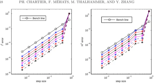
In Figure 3, the global errors of the second-order and fourth-order multi-revolution composition methods combined with the fourth-order splitting method, obtained for the linear

We first present numerical experiments for the nonlinear Klein-Gordon equation in the nonrelativistic limit regime, then we consider a stiffer problem, the nonlinear Schr¨

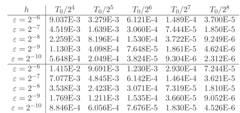
Considering (4.2) as initial data, Table 4.2 shows the failure in the spatial error by solving the original equation (1.1) in the highly oscillatory regime, where we use the

Moreover, when this splitting is coupled with spectral methods (and under some assumptions detailed in the sequel), the so-obtained method is able to capture to a very high accuracy

When applied to the numerical integration of highly oscillatory systems of differential equations, the technique benefits from the properties of standard composition methods: it

References

1. S. Alinhac, P. G´erard, Pseudo-differential Operators and Nash–Moser Theorem. Graduate Studies in Mathematics, Vol. 82, American Mathematical Society, Provi-dence, Rhode Island, 2007.
2. F. Castella, P. Chartier, F. M´ehats, A. Murua, Stroboscopic averaging for the nonlinear Schr¨odinger equation.Found. Comput. Math 15 (2015) 519–559.
3. L. Gauckler, Convergence of a split-step Hermite method for the Gross–Pitaevskii equation.IMA J. Numer. Anal. 31 (2011) 396–415.
(22)
4. Chr. Lubich, On splitting methods for Schr¨odinger-Poisson and cubic nonlinear Schr¨odinger equations.Math. Comp. 77 (2008) 2141-2153.
5. C. Muscalu, W. Schlag, Classical and multilinear harmonic analysis. Vol. II. bridge Studies in Advanced Mathematics, 138. Cambridge University Press, Cam-bridge, 2013.
6. J.A.C. Weideman, B.M. Herbst, Split-step methods for the solution of the nonlinear Schr¨odinger equation.SIAM J. Numer. Anal. 23 (1986) 485-507.
7. H. Yoshida, Construction of higher order symplectic integrators. Phys. Lett. A 150 (1990) 262–268.
Appendix A. Auxiliary results
Elementary result for periodic functions. In the sequel, we state an elementary result on the approximation by Riemann sums for periodic func-tions, see (1.6) for the definition of Fτ.
Lemma A.1. For given h > 0 and n ∈ N such that nh = T0= 1, let
(A.1) ERie(u, h) =
1 n n−1 X ℓ=0 Fℓh(u) − Z 1 0 Fτ(u)dτ
denote the error in the approximation of the integral by its Riemann sum. Then, the following estimate holds with m = ⌊σ/2⌋
(A.2) kERie(u, h)kHσ−2m ≤ 21−mπ−mζ(m)hm sup
τ ∈[0,1]k∂ m
τ Fτ(u)kHσ−2m.
Proof. Our starting point is the Fourier expansion of Fτ
X
k∈Z
ei2πkτFˆk(u).
By the definition of the Fourier coefficients, we have
Z 1
0
Fτ(u)dθ = ˆF0(u).
The numerical counterpart is 1 n n−1 X ℓ=0 Fℓh(u) = 1 n n−1 X ℓ=0 X k∈Z ei2πℓkhFˆk(u) =X k∈Z 1 n n−1X ℓ=0 ei2πkℓhFˆk(u) =X q∈Z ˆ Fnq(u). Hence, we obtain kERie(u, h)kHσ−2m ≤ X q∈Z∗ k ˆFnq(u)kHσ−2m.
Owing to the regularity of Fτ
∀ k ∈ Z∗: k ˆFk(u)kHσ−2m ≤ sup
τ ∈[0,1](2π|k|) −mk∂m
(23)
we have
kERie(u, h)kHσ−2m ≤ 2 sup
τ ∈[0,1]k∂ m τ Fτ(u)kHσ−2m X q∈N∗ (2πnq)−m = 2(2πn)−mζ(m) sup τ ∈[0,1]k∂ m τ Fτ(u)kHσ−2m.
This is the stated result.
Products and functions in Sobolev spaces. The fractional Leibniz rule for functions defined on a d-dimensional torus follows from the standard
fractional Leibniz rule for functions defined on Rd.
Lemma A.2 (See [5]). Assume s > 0, and let p, q1, q2, p1, p2 ∈ (1, ∞) be
such that 1p = p1 1 + 1 q1 = 1 p2 + 1
q2. Then, for all elements u ∈ L
p1(Td) ∩ Ws,q2(Td) and v ∈ Lp2(Td) ∩ Ws,q1(Td), the following estimate holds with constant α > 0
(A.3) kuvkWs,p ≤ αkukLp1kvkWs,q1 + αkukWs,q2kvkLp2.
The relation remains valid for exponents p ∈ [1, ∞) and p1, p2, q1, q2 ∈
(1, ∞].
The following auxiliary result is used in Section 2.
Lemma A.3. Assume σ > d2 and s ∈ [0, σ]. Then, for all elements u ∈
Hs(Td) and v ∈ Hσ(Td), the relation
(A.4) kuvkHs ≤ κkukHskvkHσ
holds. Moreover, for any function f ∈ C1(R, R) and for all elements u, v ∈
BRσ the estimate
(A.5) kf (u) − f (v)kHs ≤ α(f, R)ku − vkHs
is valid.
Proof. We recall that, for any σ > d2, the continuous Sobolev embedding
(Td) ֒→ L(Td) holds, that is kvk
L∞ ≤ c kvkHσ. Hence, in the case
s = 0, the result is obvious, since we have
kuvkL2 ≤ kukL2kvkL∞ ≤ ckukL2kvkHσ and