HAL Id: hal-02969811
https://hal.archives-ouvertes.fr/hal-02969811v2
Submitted on 19 Oct 2020
HAL is a multi-disciplinary open access
archive for the deposit and dissemination of
sci-entific research documents, whether they are
pub-lished or not. The documents may come from
teaching and research institutions in France or
abroad, or from public or private research centers.
L’archive ouverte pluridisciplinaire HAL, est
destinée au dépôt et à la diffusion de documents
scientifiques de niveau recherche, publiés ou non,
émanant des établissements d’enseignement et de
recherche français ou étrangers, des laboratoires
publics ou privés.
Patch-based CNN evaluation for bark classification
Debaleena Misra, Carlos Crispim-Junior, Laure Tougne
To cite this version:
Debaleena Misra, Carlos Crispim-Junior, Laure Tougne. Patch-based CNN evaluation for bark
clas-sification. Workshop on Computer Vision Problems in Plant Phenotyping, Aug 2020, Edinburgh,
United Kingdom. �hal-02969811v2�
classification
2
Debaleena Misra1, Carlos Crispim-Junior1[0000−0002−5577−5335], and Laure
3
Tougne1[0000−0001−9208−6275]
4
Univ Lyon, Lyon 2, LIRIS, F-69676 Lyon, France
5
{debaleena.misra,carlos.crispim-junior,laure.tougne}@liris.cnrs.fr
6
Abstract. The identification of tree species from bark images is a
chal-7
lenging computer vision problem. However, even in the era of deep
learn-8
ing today, bark recognition continues to be explored by traditional
meth-9
ods using time-consuming handcrafted features, mainly due to the
prob-10
lem of limited data. In this work, we implement a patch-based
convolu-11
tional neural network alternative for analyzing a challenging bark dataset
12
Bark-101, comprising of 2587 images from 101 classes. We propose to
ap-13
ply image re-scaling during the patch extraction process to compensate
14
for the lack of sufficient data. Individual patch-level predictions from
fine-15
tuned CNNs are then combined by classical majority voting to obtain
16
image-level decisions. Since ties can often occur in the voting process,
17
we investigate various tie-breaking strategies from ensemble-based
clas-18
sifiers. Our study outperforms the classification accuracy achieved by
19
traditional methods applied to Bark-101, thus demonstrating the
feasi-20
bility of applying patch-based CNNs to such challenging datasets.
21
Keywords: Bark classification, convolutional neural networks,
trans-22
fer learning, patch-based CNNs, image re-scaling, bicubic interpolation,
23
super-resolution networks, majority voting
24
1
Introduction
25
Automatic identification of tree species from images is an interesting and chal-26
lenging problem in the computer vision community. As urbanization grows, our 27
relationship with plants is fast evolving and plant recognition through digital 28
tools provide an improved understanding of the natural environment around 29
us. Reliable and automatic plant identification brings major benefits to many 30
sectors, for example, in forestry inventory, agricultural automation [32], botany 31
[27], taxonomy, medicinal plant research [3] and to the public, in general. In re-32
cent years, vision-based monitoring systems have gained importance in agricul-33
tural operations for improved productivity and efficiency [17]. Automated crop 34
harvesting using agricultural robotics [2] for example, relies heavily on visual 35
identification of crops from their images. Knowledge of trees can also provide 36
landmarks in localization and mapping algorithms [31]. 37
Although plants have various distinguishable physical features such as leaves, 39
fruits or flowers, bark is the most consistent one. It is available round the year, 40
with no seasonal dependencies. The aging process is also a slow one, with vi-41
sual features changing over longer periods of time while being consistent during 42
shorter time frames. Even after trees have been felled, their bark remains an 43
important identifier, which can be helpful for example, in autonomous timber 44
assessment. Barks are also more easily visually accessible, contrary to higher-45
level leaves, fruits or flowers. However, due to the low inter-class variance and 46
high intra-class variance for bark data, the differences are very subtle. Besides, 47
bark texture properties are also impacted by the environment and plant diseases. 48
Uncontrolled illumination alterations and branch shadow clutter can addition-49
ally affect image quality. Hence, tree identification from only bark images is a 50
challenging task not only for machine learning approaches [5][7][8][25] but also 51
for human experts [13]. 52
53
Recent developments in deep neural networks have shown great progress in image 54
recognition tasks, which can help automate manual recognition methods that are 55
often laborious and time consuming. However, a major limitation of deep learn-56
ing algorithms is that a huge amount of training data is required for attaining 57
good performance. For example, the ImageNet dataset [11] has over 14 million 58
images. Unfortunately, the publicly available bark datasets are very limited in 59
size and variety. Recently released BarkNet 1.0 dataset [8] with 23,000 images 60
for 23 different species, is the largest in terms of number of instances, while 61
Bark-101 dataset [25] with 2587 images and 101 different classes, is the largest 62
in terms of number of classes. The data deficiency of reliable bark datasets in 63
literature presumably explains why majority of bark identification research has 64
revolved around hand-crafted features and filters such as Gabor [4][18], SIFT 65
[9][13], Local Binary Pattern (LBP) [6][7][25] and histogram analysis [5], which 66
can be learned from lesser data. 67
68
In this context, we study the challenges of applying deep learning in bark recog-69
nition from limited data. The objective of this paper is to investigate patch-based 70
convolutional neural networks for classifying the challenging Bark-101 dataset 71
that has low inter-class variance, high intra-class variance and some classes with 72
very few samples. To tackle the problem of insufficient data, we enlarge the train-73
ing data by using patches cropped from original Bark-101 images. We propose 74
a patch-extraction approach with image re-scaling prior to training, to avoid 75
random re-sizing during image-loading. For re-scaling, we compare traditional 76
bicubic interpolation [10] with a more recent advance of re-scaling by super-77
resolution convolutional neural networks [12]. After image re-scale and patch-78
extraction, we fine-tune pre-trained CNN models with these patches. We obtain 79
patch-level predictions which are then combined in a majority voting fashion to 80
attain image-level results. However, there can be ties, i.e. more than one class 81
could get the largest count of votes, and it can be challenging when a considerable 82
number of ties occur. In our study, we apply concepts of ensemble-based classi-83
fiers and investigate various tie-breaking strategies [22][23][26][34][35] of major-84
ity voting. We validated our approach on three pre-trained CNNs - Squeezenet 85
[20], MobileNetV2 [28] and VGG16 [30], of which the first two are compact and 86
light-weight models that could be used for applications on mobile devices in the 87
future. Our study demonstrates the feasibility of using deep neural networks for 88
challenging datasets and outperforms the classification accuracy achieved using 89
traditional hand-crafted methods on Bark-101 in the original work [25]. 90
91
The rest of the paper is organised as follows. Section 2 reviews existing ap-92
proaches in bark classification. Then, section 3 explains our methodology for 93
patch-based CNNs. Section 4 describes the experimentation details. Our results 94
and insights are presented in section 5. Finally, section 6 concludes the study 95
with discussions on possible future work. 96
2
RELATED WORK
97
Traditionally, bark recognition has been studied as a texture classification prob-98
lem using statistical methods and hand-crafted features. Bark features from 160 99
images were extracted in [33] using textual analysis methods such as gray level 100
run-length method (RLM), concurrence matrices (COMM) and histogram in-101
spection. Additionally, the authors captured the color information by applying 102
the grayscale methods individually to each of the 3 RGB channels and the overall 103
performance significantly improved. Spectral methods using Gabor filters [4] and 104
descriptors of points of interests like SURF or SIFT [9][13][16] have also been 105
used for bark feature extraction. The AFF bark dataset, having 11 classes and 106
1082 bark images, was analysed by a bag of words model with an SVM classifier 107
constructed from SIFT feature points achieving around 70% accuracy [13]. 108
109
An earlier study [5] proposed a fusion of color hue and texture analysis for 110
bark identification. First the bark structure and distribution of contours (scales, 111
straps, cracks etc) were described by two descriptive feature vectors computed 112
from a map of Canny extracted edges intersected by a regular grid. Next, the 113
color characteristics were captured by the hue histogram in HSV color space as 114
it is indifferent to illumination conditions and covers the whole range of possi-115
ble bark colors with a single channel. Finally, image filtering by Gabor wavelets 116
was used to extract the orientation feature vector. An extended study on the 117
resultant descriptor from concatenation of these four feature vectors, showed 118
improved performance in tree identification when combined with leaves [4]. Sev-119
eral works have also been based on descriptors such as Local Binary Patterns 120
(LBP) and LBP-like filters [6][7][25]. Late Statistics (LS) with two state-of-art 121
LBP-like filters - Light Combination of Local Binary Patterns (LCoLBP) and 122
Completed Local Binary Pattern (CLBP) were defined, along with bark priors on 123
reduced histograms in the HSV space to capture color information [25]. This ap-124
proach created computationally efficient, compact feature vectors and achieved 125
state-of-art performance on 3 challenging datasets (BarkTex, AFF12, Bark-101) 126
with SVM and KNN classifiers. Another LBP-inspired texture descriptor called 127
Statistical Macro Binary Pattern (SMBP) attained improved performance in 128
classifying 3 datasets (BarkTex, Trunk12, AFF) [7]. SMBP encodes macrostruc-129
ture information with statistical description of intensity distribution which is 130
rotation-invariant and applies an LBP-like encoding scheme, thus being invari-131
ant to monotonic gray scale changes. 132
133
Some early works [18][19] in bark research have interestingly been attempted 134
using artificial neural networks (ANN) as classifiers. In 2006, Gabor wavelets 135
were used to extract bark texture features and applied to a radial basis proba-136
bilistic neural network (RBPNN) for classification [18]. It achieved around 80% 137
accuracy on a dataset of 300 bark images. GLCM features have also been used 138
in combination with fractal dimension features to describe the complexity and 139
self-similarity of varied scaled texture [19]. They used a 3-layer ANN classifier on 140
a dataset of 360 images having 24 classes and obtained an accuracy of 91.67%. 141
However, this was before the emergence of deep learning convolutional neural 142
networks for image recognition. 143
144
Recently, there have been few attempts to identify trees from only bark informa-145
tion using deep-learning. LIDAR scans created depth images from point clouds, 146
which were applied to AlexNet resulting in 90% accuracy, using two species only 147
- Japanese Cedar and Japanese Cypress [24]. Closer to our study with RGB 148
images, patches of bark images have been used to fine-tune pre-trained deep 149
learning models [15]. With constraints on the minimum number of crops and 150
projected size of tree on plane, they attained 96.7% accuracy, using more than 151
10,000 patches for 221 different species. However, the report lacked clarity on the 152
CNN architecture used and the experiments were performed on private data pro-153
vided by a company, therefore inaccessible for comparisons. Image patches were 154
also used for transfer-learning with ResNets to identify species from the BarkNet 155
dataset [8]. This work obtained an impressive accuracy of 93.88% for single crop 156
and 97.81% using majority voting on multiple crops. However, BarkNet is a large 157
dataset having 23,000 high-resolution images for 23 classes, which significantly 158
reduces the challenges involved. We draw inspiration from these works and build 159
on them to study an even more challenging dataset - Bark-101 [25]. 160
3
METHODOLOGY
161
Our methodology presents a plan of actions consisting of four main components: 162
Image re-scaling, patch-extraction, fine-tuning pre-trained CNNs and majority 163
voting analysis. The following sections discuss our work-flow in detail. 164
3.1 Dataset 165
In our study, we chose the Bark-101 dataset. It was developed from PlantCLEF 166
database, which is part of the ImageCLEF challenges for plant recognition [21]. 167
Bark-101 consists of a total of 2587 images (split into 1292 train and 1295 test 168
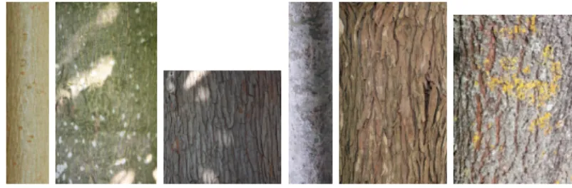
images) belonging to 101 different species. Two observations about Bark-101 ex-169
plain the difficulty level of this dataset. Firstly, these images simulate real world 170
conditions as PlantCLEF forms their database through crowdsourced initiatives 171
(for example from mobile applications as Pl@ntnet [1]). Although the images 172
have been manually segmented to remove unwanted background, Bark-101 still 173
contains a lot of noise in form of mosses, shadows or due to lighting conditions. 174
Moreover, no constraints were given for image sizes during Bark-101 preparation 175
leading to a huge variability of size. This is expected in practical outdoor set-176
tings where tree trunk diameters fluctuate and users take pictures from varying 177
distances. Secondly, Bark-101 has high intra-class variability and low inter-class 178
variability which makes classification difficult. High intra-class variability can 179
be attributed to high diversity in bark textures during the lifespan of a tree. 180
Low inter-class variability is explained by the large number of classes (101) in 181
the dataset, as a higher number of species imply higher number of visually alike 182
textures. Therefore, Bark-101 can be considered a challenging dataset for bark 183
recognition.
Fig. 1. Example images from Bark-101 dataset.
184
3.2 Patch preparation 185
In texture recognition, local features can offer useful information to the clas-186
sifier. Such local information can be obtained through extraction of patches, 187
which means decomposing the original image into smaller crops or segments. 188
Compared to semantic segmentation techniques that use single pixels as input, 189
patches allow to capture neighbourhood local information as well as reduces ex-190
ecution time. These patches are then used for fine-tuning a pre-trained CNN 191
model. Thus, the patch extraction process also helps to augment the available 192
data for training CNNs and is particularly useful when the number of images 193
per class is low, as is the case with Bark-101 dataset. 194
195
Our study focused on using a patch size of 224x224 pixels, following the de-196
fault ImageNet size standards used in most CNN image recognition tasks today. 197
However, when the range of image dimensions vary greatly within a dataset, it 198
is difficult to extract a useful number of non-overlapping patches from all im-199
ages. For example, in Bark-101, around 10 percent of the data is found to have 200
insufficient pixels to allow even a single square patch of 224x224 size. Contrary 201
to common data pre-processing for CNNs where images are randomly re-sized 202
and cropped during data loading, we propose to prepare the patches beforehand 203
to have better control in the patch extraction process. This also removes the risk 204
of extracting highly deformed patches from low-dimension images. The original 205
images are first upscaled by a given factor and then patches are extracted from 206
them. In our experiments, we applied two different image re-scaling algorithms 207
- traditional bicubic interpolation method [10] and a variant of super-resolution 208
network, called efficient sub-pixel convolutional neural network (ESPCN) [29]. 209
3.3 Image re-scaling 210
Image re-scaling refers to creating a new version of an image with new dimen-211
sions by changing its pixel information. In our study, we apply upscaling which 212
is the process of obtaining images with increased size. However, these operations 213
are not loss-less and have a trade-off between efficiency, complexity, smoothness, 214
sharpness and speed. We tested two different algorithms to obtain high-resolution 215
representation of the corresponding low-resolution image (in our context, reso-216
lution referring to spatial resolution, i.e. size). 217
Bicubic interpolation This is a classical image upsampling algorithm involv-218
ing geometrical transformation of 2D images with Lagrange polynomials, cubic 219
splines or cubic convolutions [10]. In order to preserve sharpness and image 220
details, new pixel values are approximated from the surrounding pixels in the 221
original image. The output pixel value is computed as a weighted sum of pixels 222
in the 4-by-4 pixel neighborhood. The convolution kernel is composed of piece-223
wise cubic polynomials. Compared to bilinear or nearest-neighbor interpolation, 224
bicubic takes longer time to process as more surrounding pixels are compared 225
but the resampled images are smoother with fewer distortions. As the destina-226
tion high-resolution image pixels are estimated using only local information in 227
the corresponding low-resolution image, some details could be lost. 228
resolution using sub-pixel convolutional neural network Super-229
vised machine learning methods can learn mapping functions from low-resolution 230
images to their high-resolution representations. Recent advances in deep neu-231
ral networks called Super-resolution CNN (SRCNN) [12] have shown promising 232
improvements in terms of computational performances and reconstruction accu-233
racy. These models are trained with low-resolution images as inputs and their 234
high-resolution counterparts are the targets. The first convolutional layers of 235
such neural networks perform feature extraction from the low-resolution images. 236
The next layer maps these feature maps non-linearly to their corresponding 237
high-resolution patches. The final layer combines the predictions within a spa-238
tial neighbourhood to produce the final high-resolution image. 239
Fig. 2. SRCNN architecture [12].
240
In our study, we focus on the efficient sub-pixel convolutional neural network 241
(ESPCN) [29]. In this CNN architecture, feature maps are extracted from low-242
resolution space, instead of performing the super-resolution operation in the 243
high-resolution space that has been upscaled by bicubic interpolation. Addition-244
ally, an efficient sub-pixel convolution layer is included that learns more complex 245
upscaling filters (trained for each feature map) to the final low-resolution feature 246
maps into the high-resolution output. This architecture is shown in figure 3, with 247
two convolution layers for feature extraction, and one sub-pixel convolution layer 248
which accumulates the feature maps from low-resolution space and creates the 249
super-resolution image in a single step. 250
Fig. 3. Efficient sub-pixel convolutional neural network (ESPCN) [29].
3.4 CNN classification 251
The CNN models used for image recognition in this work are 3 recent architec-252
tures: Squeezenet [20], MobileNetV2 [28] and VGG16 [30]. Since Bark-101 is a 253
small dataset, we apply transfer-learning and use the pre-trained weights of the 254
models trained on the large-scale image data of ImageNet [11]. The convolutional 255
layers are kept frozen and only the last fully connected layer is replaced with a 256
new one having random weights. We only train this layer with the dataset to 257
make predictions specific to the bark data. We skip the detailed discussion of 258
the architectures, since its beyond the scope of our study and can be found in 259
the references for the original works. 260
3.5 Evaluation metrics 261
In our study, we report two kinds of accuracy: patch-level and absolute. 262
– Patch-level accuracy - Describes performance at a patch-level, i.e. among 263
all the patches possible (taken from 1295 test images), we record what per-264
centage of patches has been correctly classified. 265
– Absolute accuracy - Refers to overall accuracy in the test data, i.e. how 266
many among 1295 test images of Bark-101 could be correctly identified. In 267
our patch-based CNN classification, we computed this by majority voting 268
using 4 variants for resolving ties, described in the following section 3.6. 269
3.6 Majority Voting 270
Majority voting [23][35] is a popular label-fusion strategy used in ensemble-based 271
classifiers [26]. We use this for combining the independent patch-level predictions 272
into image-level results for our bark classification problem. In simple majority 273
voting, the class that gets the largest number of votes among all patches is con-274
sidered the overall class label of the image. Let us assume that an image I can be 275
cropped into x parent patches and gets x1, x2, x3 number of patches classified
276
as the first, second and third classes. The final prediction class of the image is 277
taken as the class that has max(x1, x2, x3) votes, i.e. the majority voted class.
278 279
However, there may be cases when more than one class gets the largest num-280
ber of votes. There is no one major class and ties can be found, i.e. multiple 281
classes can have the highest count of votes. In our study, we examine few tie-282
breaking strategies from existing literature in majority voting [22][23][26][34][35]. 283
The most common one is Random Selection [23] of one of the tied classes, all of 284
which are assumed to be equi-probable. Another trend of tie-breaking approaches 285
relies on class priors and we tested two variants of class prior probability in our 286
study. First, by Class Proportions strategy [34] that chooses the class having the 287
higher number of training samples among the tied classes. Second, using Class 288
Accuracy (given by F1-score), the tie goes in favor of the class having a better 289
F1-score. Outside of these standard methods, more particular to neural network 290
classifiers is the breaking of ties in ensembles by using Soft Max Accumulations 291
[22]. Neural network classifiers output, by default, the class label prediction ac-292
companied by a confidence of prediction (by using soft max function) and this 293
information is leveraged to resolve ties in [22]. In case of a tie in the voting pro-294
cess, the confidences for the received votes of the tied classes, are summed up. 295
Finally, the class that accumulates the Maximum Confidence sum is selected. 296
4
EXPERIMENTS
297
4.1 Dataset 298
Pre-processing As we used pre-trained models for fine-tuning, we resized and 299
normalised all our images to the same format the network was originally trained 300
on, i.e. ImageNet standards. For patch-based CNN experiments, no size transfor-301
mations were done during training as the patches were already of size 224x224. 302
For the benchmark experiments with whole images, the images were randomly 303
re-sized and cropped to the size of 224x224 during image-loading. For data aug-304
mentation purposes, torchvision transforms were used to obtain random hori-305
zontal flips, rotations and color jittering, on all training images. 306
Patch details Non-overlapping patches of size 224x224 were extracted in a 307
sliding window manner from non-scaled original and upscaled Bark-101 images 308
(upscale factor of 4). Bark-101 originally has 1292 training images and 1295 test 309
images. After patch-extraction by the two methods, we obtain a higher count of 310
samples as shown in table 1. In our study, 25% of the training data was kept for 311
validation.
Table 1. Count of extracted unique patches from Bark-101. Source Image Train Validation Test Non-Scaled Bark-101 3156 1051 4164 Upscaled Bark-101 74799 24932 99107
312
4.2 Training details 313
We used CNNs that have been pre-trained on ImageNet. Three architectures 314
were selected - Squeezenet, MobileNetV2 and VGG16. We used Pytorch to fine-315
tune these networks with the Bark-101 dataset, starting with an initial learning 316
rate of 0.001. Training was performed over 50 epochs with the Stochastic gradi-317
ent descent (SGD) optimizer, reducing the learning rate by a factor of 0.1 every 318
7th epoch. 319
320
ESPCN was trained from scratch for a factor of 4, on the 1292 original training 321
images of Bark-101, with a learning rate of 0.001 for 30 epochs. 322
5
RESULTS AND DISCUSSIONS
323
We present our findings with the two kinds of accuracy described in section 3.5. 324
Compared to absolute accuracy, patch-level accuracy provides a more precise 325
measure of how good the classifier model is. However, for our study, it is the ab-326
solute accuracy that is of greater importance as the final objective is to improve 327
identification of bark species. It is important to note that Bark-101 is a challeng-328
ing dataset and the highest accuracy obtained in the original work on Bark-101 329
[25] was 41.9% using Late Statistics on LBP-like filters and SVM classifiers. In 330
our study, we note this as a benchmark value for comparing our performance 331
using CNNs. 332
5.1 Using whole images 333
We begin by comparing the classification accuracy of different pre-trained CNNs 334
fine-tuned with the non-scaled original Bark-101 data. Whole images were used 335
and no explicit patches were formed prior to training. Thus, training was carried 336
out on 1292 images and testing on 1295. Table 2 presents the results.
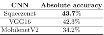
Table 2. Classification of whole images from Bark-101.
CNN Absolute accuracy Squeezenet 43.7% VGG16 42.3% MobilenetV2 34.2% 337 5.2 Using patches 338
In this section, we compare patch-based CNN classification using patches ob-339
tained by the image re-scaling methods explained in section 3.3. 340
341
In the following tables (3, 4 and 5), the column for Patch-level accuracy gives 342
the local performance, i.e how many of the test patches are correctly classified. 343
This number of test patches vary across the two methods - patches from non-344
scaled original and those from upscaled Bark-101 (see table 1). For Absolute 345
accuracy, we calculate how many of the original 1295 Bark-101 test images are 346
correctly identified, by majority voting (with 4 tie-breaking strategies) on patch-347
level predictions. Column Random selection gives results of arbitrarily breaking 348
ties by randomly selecting one of the tied classes (averaged over 5 trials). In Max 349
confidence column, the tied class having the highest soft-max accumulations is 350
selected. The last two columns use class priors for tie-breaking. Class proportions 351
selects the tied class that appears most frequently among the training samples 352
(i.e. having highest proportion) while Class F1-scores resolves ties by select-353
ing the tied class which has higher prediction accuracy (metric chosen here is 354
F1-score). The best absolute accuracy among different tie-breaking methods for 355
each CNN model, is highlighted in bold. 356
357
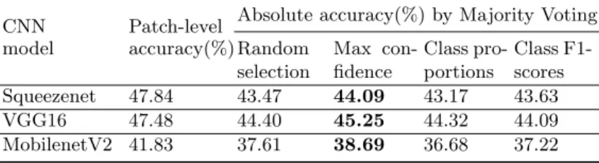
Patches from Non-Scaled Original Images Patches of size 224x224 were 358
extracted from Bark-101 data, without any re-sizing of the original images. The 359
wide variation in the sizes of Bark-101 images resulted in a minimum of zero 360
and a maximum of 9 patches possible per image. We kept all possible crops, re-361
sulting in a total of 3156 train, 1051 validation and 4164 test patches. Although 362
the number of training samples is higher than that for training with whole im-363
ages (section 5.1), only a total of 1169 original training images (belonging to 96 364
classes) allowed at least one square patch of size 224x224. Thus, there is data 365
loss as the images from which not even a single patch could be extracted were 366
excluded. Results obtained by this strategy are listed in Table 3.
Table 3. Classification of patches from non-scaled original Bark-101.
CNN Patch-level Absolute accuracy(%) by Majority Voting model accuracy(%) Random
selection Max con-fidence Class pro-portions Class F1-scores Squeezenet 47.84 43.47 44.09 43.17 43.63 VGG16 47.48 44.40 45.25 44.32 44.09 MobilenetV2 41.83 37.61 38.69 36.68 37.22 367 368
We observe that the patch-level accuracy is higher than absolute accuracy, 369
which can possibly be explained due to the data-loss. From the original test data, 370
only 1168 images (belonging to 96 classes) had dimensions that allowed at least 371
one single patch of 224x224, resulting in a total of 4164 test patches. Around 372
127 test images were excluded and by default, classified as incorrect, therefore 373
reducing absolute accuracy. For patch-level accuracy, we reported how many of 374
the 4164 test patches were correctly classified. 375
376
Patches from Upscaled Images The previous sub-section highlights the need 377
for upscaling original images, so that none is excluded from patch-extraction. 378
Here, we first upscaled all the original Bark-101 images by a factor of 4 and then 379
extracted square patches of size 224x224 from them. Figure 4 shows an example 380
pair of upscaled images and their corresponding patch samples. 381
382
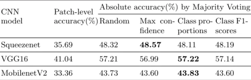
We observe that among all our experiments, better absolute accuracy is ob-383
tained when patch-based CNN classification is performed on upscaled Bark-101 384
images and shows comparable performance between both methods of upscaling 385
(bicubic or ESPCN). The best classifier performance in our study is 57.22% 386
from VGG16 fine-tuned by patches from Bark-101 upscaled by bicubic interpo-387
lation (table 4). This is a promising improvement from both the original work 388
[25] on Bark-101 (best accuracy of 41.9%) as well as the experiments using whole 389
Fig. 4. An example pair of upscaled images and sample patches from them. The left-most image has been upscaled by ESPCN and the right-left-most one by bicubic interpola-tion. Between them, sample extracted patches are shown where the differences between the two methods of upscaling become visible.
Table 4. Classification of patches from Bark-101 upscaled by bicubic interpolation.
CNN Patch-level Absolute accuracy(%) by Majority Voting model accuracy(%) Random Max
con-fidence Class pro-portions Class F1-scores Squeezenet 35.69 48.32 48.57 48.11 48.19 VGG16 41.04 57.21 56.99 57.22 57.14 MobilenetV2 33.36 43.73 43.60 43.83 43.60
Table 5. Classification of patches from Bark-101 upscaled by ESPCN.
CNN Patch-level Absolute accuracy(%) by Majority Voting model accuracy(%) Random Max
con-fidence Class pro-portions Class F1-scores Squeezenet 34.85 49.40 49.38 49.45 49.38 VGG16 39.27 55.86 55.75 55.76 55.75 MobilenetV2 32.12 42.19 41.78 41.93 41.85
images (best accuracy of 43.7% by Squeezenet, from table 2). 390
391
The comparison of tie-majority strategies shows that the differences are not 392
substantial. This is because the variations can only be visible when many ties are 393
encountered, which was not always the case for us. Table 6 lists the count of test 394
images (whole) where ties were encountered. We observe that test images in the 395
patch method with non-scaled original Bark-101, encounter 4-5 times more ties 396
than when using upscaled images (bicubic or EPSCN). Our study thus corrob-397
orates that the differences among tie-breaking strategies are more considerable 398
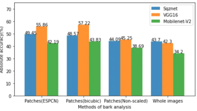
Fig. 5. Comparison of Bark-101 classification accuracy (absolute) using CNNs in this work. Best accuracy of 41.9% was obtained in the original work [25] using Late Statistics on LBP-like filters and SVM classifiers.
when several ties occur (table 3), than when fewer ties are found (tables 4 and 5). 399
However, since the total number of test images in Bark-101 is 1295, the overall 400
count of ties can still be considered low in our study. Nevertheless, we decided 401
to include this comparison to demonstrate the difficulties of encountering ties 402
in majority voting for patch-based CNN and investigate existing strategies to 403
overcome this. It is interesting to observe (in table 3) that for patches extracted 404
from non-scaled original Bark-101 (where there is a higher number of ties), the 405
best tie-breaking strategy is the maximum confidence sum, as affirmed in [22] 406
where the authors had tested it on simpler datasets (having a maximum of 26 407
classes in the Letter dataset) taken from the UCI repository [14].
Table 6. Count of test images showing tied classes in majority voting.
Patch Method Squeezenet VGG16 MobilenetV2 Non-Scaled Original 217 283 274 Upscaled by Bicubic 52 45 45 Upscaled by ESPCN 50 46 63
408
To summarise, we present few important insights. First, when the total count of 409
training samples is low, patch-based image analysis can improve accuracy due 410
to better learning of local information and also since the total count of training 411
samples increases. Second, image re-scaling invariably introduces distortion and 412
reduces the image quality, hence patches from upscaled images have a loss of fea-413
ture information. As expected, patch-level accuracy is lower when using patches 414
from upscaled images (tables 4 and 5), compared to that of patches from non-415
scaled original images having more intact features (table 3). However, we also 416
observe that absolute accuracy falls sharply for patches taken from non-scaled 417
original Bark-101. This is because several of the original images have such low 418
image dimensions, that no patch formation was possible at all. Therefore, all 419
such images (belonging to 5 classes, see section 5.2 for details) were by default 420
excluded from our consideration, resulting in low absolute accuracy across all 421
the CNN models tested. Thus, we infer that for datasets having high diversity 422
and variation of image dimensions, upscaling before patch-extraction can ensure 423
better retention and representation of data. Finally, we also observe that it is 424
useful to examine tie-breaking strategies in majority voting compared to rely-425
ing on simple random selection. These strategies are particularly significant if a 426
considerable number of ties are encountered. 427
6
CONCLUSION AND FUTURE WORK
428
Our study demonstrates the potential of using deep learning for studying chal-429
lenging datasets such as Bark-101. For a long time, bark recognition has been 430
treated as a texture classification problem and traditionally solved using hand-431
crafted features and statistical analysis. A patch-based CNN classification ap-432
proach can automate bark recognition greatly and reduce the efforts required 433
by time-consuming traditional methods. Our study shows its effectiveness by 434
outperforming accuracy on Bark-101 from traditional methods. An objective 435
of our work was also to incorporate current trends in image re-scaling and 436
ensemble-based classifiers in this bark analysis, to broaden perspectives in the 437
plant vision community. Thus, we presented recent approaches in re-scaling by 438
super-resolution networks and several tie-breaking strategies for majority voting 439
and demonstrated their impact on performance. Super-resolution networks have 440
promising characteristics to counter-balance the degradation introduced due to 441
re-scaling. Although for our study with texture data as bark, its performance 442
was comparable to traditional bicubic interpolation, we hope to investigate its 443
effects on other plant data in future works. It would also be interesting to de-444
rive inspiration from patch-based image analysis in medical image segmentation 445
where new label fusion methods are explored to integrate location information of 446
patches for image-level decisions. In future works, we intend to accumulate new 447
state-of-art methods and extend the proposed methodology to other plant or-448
gans and develop a multi-modal plant recognition tool for effectively identifying 449
tree and shrub species. We will also examine its feasibility on mobile platforms, 450
such as smart-phones, for use in real-world conditions. 451
ACKNOWLEDGEMENTS
452
This work has been conducted under the framework of the ReVeRIES project 453
(Reconnaissance de V´eg´etaux R´ecr´eative, Interactive et Educative sur Smart-454
phone) supported by the French National Agency for Research with the reference 455
ANR15-CE38-004-01. 456
References
457
1. Affouard, A., Go¨eau, H., Bonnet, P., Lombardo, J.C., Joly, A.: Pl@ntNet app in
458
the era of deep learning. In: ICLR: International Conference on Learning
Repre-459
sentations. Toulon, France (Apr 2017)
460
2. Barnea, E., Mairon, R., Ben-Shahar, O.: Colour-agnostic shape-based 3d fruit
de-461
tection for crop harvesting robots. Biosystems Engineering 146, 57–70 (2016)
462
3. Begue, A., Kowlessur, V., Singh, U., Mahomoodally, F., Pudaruth, S.: Automatic
463
recognition of medicinal plants using machine learning techniques. International
464
Journal of Advanced Computer Science and Applications 8(4), 166–175 (2017)
465
4. Bertrand, S., Ameur, R.B., Cerutti, G., Coquin, D., Valet, L., Tougne, L.: Bark
466
and leaf fusion systems to improve automatic tree species recognition. Ecological
467
Informatics 46, 57–73 (2018)
468
5. Bertrand, S., Cerutti, G., Tougne, L.: Bark Recognition to Improve Leaf-based
469
Classification in Didactic Tree Species Identification. In: VISAPP 2017 - 12th
470
International Conference on Computer Vision Theory and Applications. Porto,
471
Portugal (Feb 2017)
472
6. Boudra, S., Yahiaoui, I., Behloul, A.: A comparison of multi-scale local binary
pat-473
tern variants for bark image retrieval. In: Battiato, S., Blanc-Talon, J., Gallo, G.,
474
Philips, W., Popescu, D., Scheunders, P. (eds.) Advanced Concepts for Intelligent
475
Vision Systems. pp. 764–775. Springer International Publishing, Cham (2015)
476
7. Boudra, S., Yahiaoui, I., Behloul, A.: Plant identification from bark: A texture
477
description based on statistical macro binary pattern. In: 2018 24th International
478
Conference on Pattern Recognition (ICPR). pp. 1530–1535. IEEE (2018)
479
8. Carpentier, M., Gigu`ere, P., Gaudreault, J.: Tree species identification from bark
480
images using convolutional neural networks. In: 2018 IEEE/RSJ International
Con-481
ference on Intelligent Robots and Systems (IROS). pp. 1075–1081. IEEE (2018)
482
9. Cerutti, G., Tougne, L., Sacca, C., Joliveau, T., Mazagol, P.O., Coquin, D.,
Vaca-483
vant, A.: Late Information Fusion for Multi-modality Plant Species Identification.
484
In: Conference and Labs of the Evaluation Forum. p. Working Notes. Valencia,
485
Spain (Sep 2013)
486
10. De Boor, C.: Bicubic spline interpolation. Journal of mathematics and physics
487
41(1-4), 212–218 (1962)
488
11. Deng, J., Dong, W., Socher, R., Li, L.J., Li, K., Fei-Fei, L.: Imagenet: A
large-489
scale hierarchical image database. In: 2009 IEEE conference on computer vision
490
and pattern recognition. pp. 248–255 (2009)
491
12. Dong, C., Loy, C.C., He, K., Tang, X.: Learning a deep convolutional network for
492
image super-resolution. In: Fleet, D., Pajdla, T., Schiele, B., Tuytelaars, T. (eds.)
493
Computer Vision – ECCV 2014. pp. 184–199. Springer International Publishing,
494
Cham (2014)
495
13. Fiel, S., Sablatnig, R.: Automated identification of tree species from images of the
496
bark, leaves or needles. In: 16th Computer Vision Winter Workshop. Mitterberg,
497
Austria (Feb 2011)
498
14. Frank, A.: Uci machine learning repository. http://archive. ics. uci. edu/ml (2010)
499
15. Ganschow, L., Thiele, T., Deckers, N., Reulke, R.: Classification of tree species
500
on the basis of tree bark texture. International Archives of the Photogrammetry,
501
Remote Sensing and Spatial Information Sciences-ISPRS Archives 42(W13) (2019)
502
16. Go¨eau, H., Joly, A., Bonnet, P., Selmi, S., Molino, J.F., Barth´el´emy, D., Boujemaa,
503
N.: LifeCLEF Plant Identification Task 2014. In: Cappellato, L., Ferro, N., Halvey,
504
M., Kraaij, W. (eds.) CLEF: Conference and Labs of the Evaluation Forum. vol.
505
CEUR Workshop Proceedings, pp. 598–615. Sheffield, United Kingdom (Sep 2014)
17. Hemming, J., Rath, T.: Pa—precision agriculture: computer-vision-based weed
507
identification under field conditions using controlled lighting. Journal of
agricul-508
tural engineering research 78(3), 233–243 (2001)
509
18. Huang, Z.K., Huang, D.S., Du, J.X., Quan, Z.H., Guo, S.B.: Bark classification
510
based on gabor filter features using rbpnn neural network. In: International
con-511
ference on neural information processing. pp. 80–87. Springer (2006)
512
19. Huang, Z.K., Huang, D.S., Du, J.X., Quan, Z.H., Guo, S.B.: Bark classification
513
based on gabor filter features using rbpnn neural network. In: International
con-514
ference on neural information processing. pp. 80–87. Springer (2006)
515
20. Iandola, F.N., Han, S., Moskewicz, M.W., Ashraf, K., Dally, W.J., Keutzer, K.:
516
Squeezenet: Alexnet-level accuracy with 50x fewer parameters and¡ 0.5 mb model
517
size. arXiv preprint arXiv:1602.07360 (2016)
518
21. ImageCLEF: Plantclef 2017 (accessed on 2020-04-15), https://www.imageclef.
519
org/lifeclef/2017/plant
520
22. Kokkinos, Y., Margaritis, K.G.: Breaking ties of plurality voting in ensembles of
521
distributed neural network classifiers using soft max accumulations. In: IFIP
In-522
ternational Conference on Artificial Intelligence Applications and Innovations. pp.
523
20–28. Springer (2014)
524
23. Malmasi, S., Dras, M.: Native language identification using stacked generalization.
525
arXiv preprint arXiv:1703.06541 (2017)
526
24. Mizoguchi, T., Ishii, A., Nakamura, H., Inoue, T., Takamatsu, H.: Lidar-based
indi-527
vidual tree species classification using convolutional neural network. In:
Videomet-528
rics, Range Imaging, and Applications XIV. vol. 10332, p. 103320O. International
529
Society for Optics and Photonics (2017)
530
25. Ratajczak, R., Bertrand, S., Crispim-Junior, C.F., Tougne, L.: Efficient Bark
531
Recognition in the Wild. In: International Conference on Computer Vision Theory
532
and Applications (VISAPP 2019). Prague, Czech Republic (Feb 2019)
533
26. Rokach, L.: Ensemble-based classifiers. Artificial Intelligence Review 33(1-2), 1–39
534
(2010)
535
27. Sa Junior, J.J.d.M., Backes, A.R., Rossatto, D.R., Kolb, R.M., Bruno, O.M.:
Mea-536
suring and analyzing color and texture information in anatomical leaf cross
sec-537
tions: an approach using computer vision to aid plant species identification. Botany
538
89(7), 467–479 (2011)
539
28. Sandler, M., Howard, A., Zhu, M., Zhmoginov, A., Chen, L.C.: Mobilenetv2:
In-540
verted residuals and linear bottlenecks. In: Proceedings of the IEEE conference on
541
computer vision and pattern recognition. pp. 4510–4520 (2018)
542
29. Shi, W., Caballero, J., Husz´ar, F., Totz, J., Aitken, A.P., Bishop, R., Rueckert,
543
D., Wang, Z.: Real-time single image and video super-resolution using an efficient
544
sub-pixel convolutional neural network. In: Proceedings of the IEEE conference on
545
computer vision and pattern recognition. pp. 1874–1883 (2016)
546
30. Simonyan, K., Zisserman, A.: Very deep convolutional networks for large-scale
547
image recognition. In: Bengio, Y., LeCun, Y. (eds.) 3rd International Conference
548
on Learning Representations, ICLR 2015, San Diego, CA, USA, May 7-9, 2015,
549
Conference Track Proceedings (2015)
550
31. Smolyanskiy, N., Kamenev, A., Smith, J., Birchfield, S.: Toward low-flying
au-551
tonomous mav trail navigation using deep neural networks for environmental
552
awareness. In: 2017 IEEE/RSJ International Conference on Intelligent Robots and
553
Systems (IROS). pp. 4241–4247. IEEE (2017)
554
32. Tian, H., Wang, T., Liu, Y., Qiao, X., Li, Y.: Computer vision technology in
555
agricultural automation—a review. Information Processing in Agriculture 7(1),
556
1–19 (2020)
33. Wan, Y.Y., Du, J.X., Huang, D.S., Chi, Z., Cheung, Y.M., Wang, X.F., Zhang,
558
G.J.: Bark texture feature extraction based on statistical texture analysis. In:
Pro-559
ceedings of 2004 International Symposium on Intelligent Multimedia, Video and
560
Speech Processing, 2004. pp. 482–485. IEEE (2004)
561
34. Woods, K., Kegelmeyer, W.P., Bowyer, K.: Combination of multiple classifiers
562
using local accuracy estimates. IEEE transactions on pattern analysis and machine
563
intelligence 19(4), 405–410 (1997)
564
35. Xu, L., Krzyzak, A., Suen, C.Y.: Methods of combining multiple classifiers and
565
their applications to handwriting recognition. IEEE transactions on systems, man,
566
and cybernetics 22(3), 418–435 (1992)