Consolidation of Empirics for Calculation of VIV Response
The MIT Faculty has made this article openly available.
Please share
how this access benefits you. Your story matters.
Citation
Voie, Per, Jie Wu, Themistocles L. Resvanis, Carl M. Larsen, J. Kim
Vandiver, Michael Triantafyllou, and Rolf Baarholm. “Consolidation
of Empirics for Calculation of VIV Response.” ASME 2017 36th
International Conference on Ocean, Offshore and Arctic Engineering,
25-30 June, 2017, Trondheim, Norway, ASME, 2017.
As Published
http://dx.doi.org/10.1115/OMAE2017-61362
Publisher
ASME International
Version
Final published version
Citable link
http://hdl.handle.net/1721.1/120746
Terms of Use
Article is made available in accordance with the publisher's
policy and may be subject to US copyright law. Please refer to the
publisher's site for terms of use.
CONSOLIDATION OF EMPIRICS FOR CALCULATION OF VIV RESPONSE
Per Voie DNV GL Trondheim, Norway Jie Wu SINTEF Ocean1 Trondheim, Norway Themistocles L. Resvanis MIT, Department of MechanicalEngineering Cambridge, MA, USA Carl M. Larsen
NTNU, Department of Marine Technology
Trondheim, Norway
J. Kim Vandiver MIT, Department of Mechanical
Engineering Cambridge, MA, USA
Michael Triantafyllou MIT, Department of Mechanical
Engineering Cambridge, MA, USA Rolf Baarholm
Statoil Trondheim, Norway ABSTRACT
The present paper consolidates available experimental results for both sub-critical and critical Reynolds numbers and varying surface roughness and formulates a coefficient excitation model that aims at unbiased response estimates when using semi-empirical VIV prediction programs. A simplified procedure is suggested to account for higher order effects when relevant.
The paper discusses the use of a modified coefficient excitation model with the objective of capturing or correctly reflecting certain specific features that have been observed in sub-critical and supercritical VIV experiments.
The first part of this paper shows how the available low Reynolds number hydrodynamic data that currently forms the basis for most semi-empirical prediction software needs to be modified to correctly reflect the available experimental observations at sub-critical Reynolds numbers.
The latter part of this paper looks at the available high Reynolds experimental data and suggests ways whereby the previously identified force coefficient database might be modified to reflect what is currently known about the VIV response of smooth and rough surfaced cylinders in the critical and super-critical Reynolds regimes.
NOMENCLATURE
VIV Vortex induced vibration
CF Cross-flow
IL In-line
1 Formerly MARINTEK. SINTEF Ocean from January 2017 through an internal merger in the SINTEF Group.
Re Reynolds number
𝐶𝐶𝑑𝑑 Drag coefficient
𝐶𝐶𝑒𝑒 Excitation (lift) coefficient
𝐶𝐶𝑎𝑎 Added mass coefficient
𝐴𝐴 Displacement amplitude (m)
D Diameter
k surface roughness 𝑈𝑈 Towing speed (m/s)
𝑓𝑓𝑜𝑜𝑜𝑜𝑜𝑜 Oscillation frequency of the test cylinder
(Hz)
𝑓𝑓̅ Non-dimensional (normalized) frequency, 𝑓𝑓̅ =𝑓𝑓𝑜𝑜𝑜𝑜𝑜𝑜𝐷𝐷
𝑈𝑈
𝑈𝑈𝑟𝑟 Reduced velocity, 𝑈𝑈𝑟𝑟=𝑓𝑓𝑜𝑜𝑜𝑜𝑜𝑜𝑈𝑈𝐷𝐷
INTRODUCTION Background
Understanding the level of safety in a riser system against fatigue damage from VIV is an important issue for operators. Though a significant effort has been made over the last two decades to develop new VIV prediction models or to improve existing ones, it is still obvious that deterministic estimates of full scale riser VIV fatigue damage will include large inherent uncertainties. Besides uncertainties due to lack of knowledge of the ocean currents generating VIV, much uncertainty is linked to the amount and relevance of data available to understand, characterize and capture the broad complexity of the phenomenon of VIV. In addition, the complex structure of the Proceedings of the ASME 2017 36th International Conference on Ocean, Offshore and Arctic Engineering OMAE2017 June 25-30, 2017, Trondheim, Norway
OMAE2017-61362
prediction models is also adding to the uncertainty. If not used right, the models will give inconsistent results with significant scatter. Earlier studies indicate that response estimates are very sensitive to the empirical basis for the estimates, software specific implementations of it, and assumptions/idealizations necessary for frequency domain prediction models. In practice, response estimates of a structure provided by different engineers may vary by several orders of magnitude. This is obviously not adequate. To determine a single rational design fatigue factor for practical application with different types of risers it is a prerequisite to have a well-defined, consistent and robust procedure yielding unbiased response estimates. Such a procedure is currently not available. Much work has been carried out the last two decades: performing experiments, developing prediction models and software. But still we struggle to achieve reliable response estimates for industry projects. Typically, we struggle with problems like:
• Finding the right empirical data for the problem • Explaining deviations of 1-2 orders of magnitudes
between different software and or when applying different parameter settings for a single software • Selecting a rational design fatigue factor We consider the reasons to be:
• There is not a single empirical data set that fits all problems
• Various VIV prediction programs apply different empirical models based on different experiments (different setup, surface roughness, flow regime etc.) • Some software considers higher order effects whilst
another do not
With these differences a successful calibration of rational safety factors for VIV is far-fetched.
With support from the Norwegian Deepwater Program, the partners: MIT, SINTEF Ocean, NTNU and DNV GL have collaborated to consolidate available empirical data and best practices for VIV response prediction.
The work on consolidating the empirical basis is emphasized in the current paper.
Objective
The main objective of the work has been to provide a consistent empirical basis applicable for top tensioned and compliant, rigid and flexible pipes. A fundamental presumption is that the empirical basis aims at unbiased estimates of response at the primary frequency.
The information included in this paper forms just a small part of a much larger document currently being prepared by DNV-GL and titled “Guideline on analysis of vortex-induced vibrations in risers and umbilicals” which includes best practices on structural modelling, current profile description, heave induced VIV, fatigue calculation and VIV suppression. This
study is motivated by the desire to understand and eventually reduce the considerable variation that is often seen today in VIV predictions. The goal is to consolidated the most important information currently available in the literature and offer engineers the necessary guidance so that they can approach VIV modeling in a systematic manner.
THE CONSOLIDATED EMPIRICAL MODEL General
A model for cross-flow excitation forces at sub-critical flow regimes is created by systematically adjusting the original small scale rigid cylinder VIV derived coefficients until the empirical VIV prediction program(s) can create satisfactory predictions of larger scale elastic pipe experiments. The characteristic values of the excitation coefficients in this model are consistent with numerical and experimental estimates for the excitation coefficients of pipes with combined cross-flow and in-line VIV responses.
This model is further used as a base model to develop cross-flow excitation force coefficients for critical and super-critical flow regimes. Characteristic values of VIV responses found from model test at prototype Reynolds number are used to construct scaling parameters, which scale the sub-critical data to obtain a realistic model at higher Re and various roughness ratios. The key elements of the empirical model are:
• Constant added mass of 1.0
• Venugopal's damping model (Venugopal, 1996) • Effects from in-line oscillations on cross-flow
oscillations are accounted for in a conservative fashion • The effects from Reynolds number and surface
roughness on the magnitude of the excitation
coefficients and the maximum response are accounted for.
• The effect of auxiliary lines, e.g. booster lines on marine risers, depends significantly on flow direction. For the most onerous direction the excitation force is similar as for a bare pipe (Lie, Braaten, Szwalek, Russo, & Baarholm, Drilling riser VIV test with protorype Reynolds numbers, 2013) .
• The excitation force coefficients are not adjusted to account for higher order response (higher harmonics). Stress magnification factors are suggested to account for higher order VIV when relevant.
CF excitation coefficient model in sub-critical Re regime
Observations of VIV responses of a rigid/elastic pipe
Listed below are some observations regarding the VIV response of rigid and elastic pipes undergoing VIV. The empirical basis
developed should reflect the most important of these key findings.
1. Maximum CF A/D is about 0.9 at reduced velocity (𝑉𝑉𝑟𝑟= 𝑈𝑈 (𝑓𝑓⁄ 𝑜𝑜𝑜𝑜𝑜𝑜𝐷𝐷)) 5.6 when a rigid pipe is free to oscillate in CF direction, but IL motion is restricted. (Sarpkaya, 2004)
2. When an elastic pipe is freely oscillating in both IL and CF direction, the maximum CF A/D reaches about 1.5 and its position shifts to 𝑉𝑉𝑟𝑟= 7. The reduced velocity for the maximum IL response is about 5 and the corresponding CF A/D is about 0.9. (Sarpkaya, 2004)
3. Inverse analysis of response data from model tests with elastic pipes (e.g. rotating rig, Shell 38m, NDP 38m) show that the maximum excitation coefficient, Ce, can reach about 1.4 at non-dimensional frequency
(𝑓𝑓̂ = 𝑓𝑓𝑜𝑜𝑜𝑜𝑜𝑜𝐷𝐷 𝑈𝑈⁄ ) about 0.13-0.14. The secondary excitation zone is located at 𝑓𝑓̂~0.2. These force coefficients are also influenced by the motion orbits along the flexible pipe. (Wu J. , 2011) (Wu, Lie, Larsen, Liapis.S., & Baarholm, 2016)
4. Inverse analysis of the Hanøytangen test response data shows that the maximum value of the excitation coefficient is reduced to about 0.8 when there are multiple response frequencies along the pipe. (Wu J. , 2011).
5. DNS simulation (Bourget, G.E., & M.S., 2013) of a elastic pipe reveals the importance of motion phase angle for describing IL and CF interaction at single or multiple shedding frequencies. These findings are consistent with results from model tests listed in item 3 and 4.
6. The Ce curve and St number in SHEAR7 need to be
adjusted as a function of Reynolds number to give a better fit to the Shell 38m test data (Resvanis, 2014). The maximum Ce is found to be 1.09 and the lowest St
number is about 0.13 (equivalent to non-dimensional frequency with the terminology used herein). The maximum amplitude ratio A/D is about 1.22 when Ce
equals to zero.
In summary, the following two effects were observed from free CF and IL response tests with spring-mounted rigid pipes and elastic/flexible pipes when compared to hydrodynamic data from
pure CF model tests. Firstly, the location of the maximum A/D and/or Ce shifts to higher reduced velocity (equivalent to lower
non-dimensional response frequency). Secondly, both the magnitude of Ce and maximum A/D increase. Therefore, a CF
force coefficient model that can consider these two factors is desired.
Methodology to derive an adjusted set of CF excitation parameters
The empirical basis was obtained by systematically varying or adjusting the original hydrodynamic database present in the empirical VIV prediction software until the comparisons with a chosen elastic pipe VIV model test data were satisfactory. The excitation coefficient Ce is a function of amplitude ratio,
A/D, for a given non-dimensional frequency, 𝑓𝑓̂. When used with empirical VIV prediction software this curve is often postulated by two sections of 2nd order polynomial curves as shown in
Figure 1. In this figure, three points (A, B, C) are used to define these curves and only four numeric values need to be specified (2 coordinates for point B and 1 for each of points A and C) because of the way that these curves are defined. The values of these points can be tabulated for different non-dimensional response frequency. An example is presented in Figure 2.
Figure 1 Illustration of a typical excitation coefficient
curve
Figure 2 An example of parameters defining excitation
coefficient curve for different non-dimensional
frequencies
The method which was used to obtain the adjusted set of parameters is briefly outlined below. The six parameters that are most important to controlling the shape of the Ce vs. A/D vs. 𝑓𝑓̂
surface (i.e. the coefficient database) were systematically varied by applying scaling parameters to each one of these. The six parameters consisted of the 4 numeric values necessary for specifying an Ce vs. A/D curve at each non-dimensional
frequency and the actual location of the two non-dimensional frequencies were peak lift is observed in the original hydrodynamic database ( 𝑓𝑓̂~0.18 and 𝑓𝑓̂~0.2).
Figure 3 Principles of scaling the excitation coefficient
curve
By systematically varying the parameters listed above and comparing the VIV predictions generated by the empirical software with the experimental measurements from the elastic pipe model tests the most suitable parameters were identified. In this study, the 38m NDP tests were chosen as the reference model test data. The obtained parameters are presented in Figure 4 which shows that the maximum Ce is about 1.44 at 𝑓𝑓̂ = 0.13
and the maximum A/D when Ce equals to zero is about 1.35.
Because such large limit-cycle amplitudes are not typically observed in elastic pipe VIV model tests, this value was subsequently reduced to 1.2.
The maximum Ce in the secondary excitation region, 1.17, and
the corresponding A/D at zero lift, 0.87, agree with the results from inverse analysis and the observations of rigid pipe tests. Based on the new model whose coefficients are shown in Figure 4 a new map of excitation coefficients versus response amplitude and non-dimensional response frequency is shown in Figure 5. The contour plot with Gopalkrishnan's data which formed the original hydrodynamic database for many of the semi-empirical programs is presented in Figure 6 for comparison.
The key differences are the overall increase of the limit cycle amplitudes (Ce=0 contours) and the shift of the Ce peak to a lower nondimensional frequency value. Both necessary in order to correctly capture the large response amplitudes observed and the slightly lower dimensionless frequencies at which these occurred in the 38m NDP flexible pipe/cylinder experiments.
Figure 4 Obtained adjusted set of parameters based
on NDP 38m data
Figure 5 CF excitation coefficient contour plots
generated the adjusted set of parameters based on
NDP 38m data
Figure 6 CF excitation coefficient contour plots
reconstructed from rigid pipe pure CF test data
(Gopalkrishnan, Vortex-Induced Forces on Oscillating
Bluff Cylinders, 1992)
Benchmark study of the adjusted set of excitation coefficients
The adjusted set of the excitation coefficient parameters is used to predict VIV responses and compare with results from several different elastic pipe model tests, which are currently available for study. The characteristics of the model tests are summarized in the table below.
Figure 7 and Figure 8 show how the revised excitation coefficient database results in more accurate predictions of both the excited frequency and the resulting fatigue damage for the
NDP 38m dataset when compared to predictions using the default parameters. Note particularly how the shift of the maximum positive excitation coefficient from a value of f*~0.17 in the original excitation database (Figure 2) to a smaller value of f*~0.13 in the adjusted parameter set (Figure 4) leads to smaller predicted excitation frequencies which are much closer to the frequencies observed in the model tests as shown in Figure 7. Similarly, the larger limit-cycle amplitude and maximum coefficient identified in the adjusted parameter set and discussed previously result in predictions with larger fatigue damage rates which are also closer to the measured values shown in Figure 8
Table 1 Summary of model tests
Model test* Mode Stiffness Response Frequency
NDP 38m 3-14 Tension dominated Dominated by one frequency at low mode cases Time/space sharing observed at higher mode cases
Rotating Rig 3-5 Tension dominated Dominated by one frequency Hanøytangen 8-25 Significant bending
stiffness Time/space sharing RotRig(EM10 m) 1-8 Significant bending stiffness Time/space sharing *Only linearly sheared flow tests are considered
The NDP 38m test pipe and its experimental setup is very like the Shell 38m test (Pipe2). It is therefore expected that this set of parameters can also give satisfactory prediction for Shell 38m test.
Good agreement between predictions and tests data for the rotating rig test is also achieved with the same adjusted parameter set as shown in Figure 10. Over-prediction of the response measured in the ExxonMobil and Hanøytangen experiments is observed though the dominating frequency and mode are reasonably well predicted. This seems to be related to that fact that multi-frequency responses are more pronounced in the latter two tests in addition to their higher bending stiffness the maximum excitation coefficient is expected to be significantly lower for these tests.
As discussed in the introduction, one of the motivations behind this collaborative project was to understand and minimize the discrepancies in VIV predictions that are often observed when different prediction programs are used to model the same experimental dataset.
It is clear that minimizing these variations in the predictions requires that the programs use the same hydrodynamic excitation database and that efforts are made by the users to choose settings
that will keep the modelling assumptions as similar as possible between programs. When this is done the commonly used semi empirical VIV predictions programs can produce very similar predictions.
This is illustrated in Figure 9 and Figure 10 which include SHEAR7 predictions that are very like the VIVANA predictions. Note that, it is inevitable that some discrepancies will exist when comparing so many tests and the comparison between the two programs has not been included here to promote one over the other but rather to emphasize that when the appropriate steps are taken and common modelling assumptions and coefficient databases are used the predictions generated can be indeed be in close agreement.
VIVA predictions are not shown here but the same empirical basis we expect similar predictions as for Shear7 and VIVANA.
Figure 7 Dominating frequency prediction for 22 NDP 38m sheared flow cases.
Figure 8 Maximum fatigue damage NDP 38m pipe test. Comparison of VIVANA with default and
adjusted parameters and measurements (the higher harmonics haven been filtered out of the measured data)
Figure 9 Maximum fatigue damage in NDP 38m pipe
test. Comparison of predictions (Shear7 and VIVANA)
versus measurements.
Figure 10 Maximum average displacement in Rotating
rig test. Comparison of predictions (Shear7 and
VIVANA) versus measurements.
CF excitation force coefficient model in prototype Re regime
General
The excitation coefficient model that was created for the sub-critical Reynolds regime and described in the preceding section can be used as a base model for predictions at higher Reynolds numbers after the appropriate adjustments are made. The characteristic values of the model will need to be scaled for Reynolds number and roughness.
It is known that both the response amplitude ratio and the excitation coefficient are significantly influenced by in-line response, Reynolds number and surface roughness at prototype Reynolds. However, most of the high Re VIV model tests were carried out without IL motions. A CF excitation coefficient model that does not depend on the IL response amplitude is considered as a realistic model based on the available data.
𝐶𝐶𝐶𝐶𝐶𝐶𝐶𝐶= 𝑓𝑓�𝐴𝐴/𝐷𝐷𝐶𝐶𝐶𝐶, 𝑓𝑓̂𝐶𝐶𝐶𝐶, 𝑅𝑅𝐶𝐶, 𝑘𝑘� (1)
It is still difficult to obtain a full experimental excitation coefficient model covering a similar parameter range as for low Re values due to limited data available. Furthermore, The complexity of including roughness as a parameter makes the required number of tests even higher than for low Re testing. It is therefore proposed to create an excitation coefficient model for high Re values by scaling the available sub-critical Re data in a way that will reflect the available high Re experimental observations. The method is illustrated in the figure below. The original Ce curve is multiplied by two scaling parameters, refer
to Figure 3. The scaling parameters must be identified from prototype Re data such as (Yin, Wu, Lie, Baarholm, & Larsen, 2015) or other relevant prototype scale Re data.
Predictions of response amplitude for risers in uniform flows or very weakly sheared currents with small amounts of damping are mostly affected by the magnitude of A/D when Ce=0 (the
cross-over point or limit cycle amplitude). In fact, the actual magnitudes of the rest of the Ce curve will not make any
difference to the predicted response amplitude. Whereas riser predictions in sheared flows with significant amounts of damping will be mostly controlled by the shape and magnitude of the Ce curve between Ce,max and Ce=0.
The scaling procedure consists of 3 steps described in the following sections
Step 1: Amplitude ratio modification
The maximum dimensionless response amplitude is a function of Reynolds number, roughness ratio and reduced velocity. For response predictions at different Reynolds number or for pipes with different roughness ratio, the amplitude ratio modification factor is modified per existing experimental results. The amplitude ratio modification factor is defined as
𝜸𝜸𝑨𝑨/𝑫𝑫(𝑹𝑹𝑹𝑹,𝒌𝒌/𝑫𝑫) =𝑨𝑨/𝑫𝑫𝑨𝑨/𝑫𝑫𝑪𝑪𝑹𝑹=𝟎𝟎,𝒎𝒎𝒎𝒎𝒎𝒎�𝒇𝒇�, 𝑹𝑹𝑹𝑹, 𝒌𝒌 𝑫𝑫⁄ �
𝑪𝑪𝑹𝑹=𝟎𝟎,𝒎𝒎𝒎𝒎𝒎𝒎�𝒇𝒇�, 𝑹𝑹𝑹𝑹𝒃𝒃𝒎𝒎𝒃𝒃𝑹𝑹, 𝒌𝒌/𝑫𝑫𝒃𝒃𝒎𝒎𝒃𝒃𝑹𝑹� (2)
where 𝐴𝐴/𝐷𝐷𝐶𝐶𝑒𝑒=0,𝑚𝑚𝑎𝑎𝑚𝑚�𝑓𝑓̂, 𝑅𝑅𝐶𝐶, 𝑘𝑘 𝐷𝐷⁄ � is the maximum response amplitude ratio for a specified 𝑅𝑅𝐶𝐶 and 𝑘𝑘 𝐷𝐷⁄ , 𝐴𝐴/ 𝐷𝐷𝐶𝐶𝑒𝑒=0,𝑚𝑚𝑎𝑎𝑚𝑚�𝑓𝑓̂, 𝑅𝑅𝐶𝐶𝑏𝑏𝑎𝑎𝑜𝑜𝑒𝑒, 𝑘𝑘/𝐷𝐷𝑏𝑏𝑎𝑎𝑜𝑜𝑒𝑒� is the maximum response
amplitude ratio of the base parameters.
The amplitude ratio modification factor can be applied on the (𝐴𝐴/𝐷𝐷)𝐶𝐶𝑒𝑒,𝐶𝐶𝐶𝐶=𝑚𝑚𝑎𝑎𝑚𝑚 and (𝐴𝐴/𝐷𝐷)𝐶𝐶𝑒𝑒,𝐶𝐶𝐶𝐶=0.
𝐴𝐴/𝐷𝐷�𝑓𝑓̂, 𝑅𝑅𝑒𝑒, 𝑘𝑘 𝐷𝐷⁄ � = 𝐴𝐴/𝐷𝐷�𝑓𝑓̂, 𝑅𝑅𝐶𝐶𝑑𝑑𝑒𝑒𝑓𝑓, 𝑘𝑘/𝐷𝐷𝑑𝑑𝑒𝑒𝑓𝑓�𝛾𝛾𝐴𝐴/𝐷𝐷(𝑅𝑅𝑒𝑒, 𝑘𝑘/𝐷𝐷) (3)
The blue line in Figure 3 shows the excitation coefficient curve after applying a 𝛾𝛾𝐴𝐴/𝐷𝐷(𝑅𝑅𝐶𝐶, 𝑘𝑘/𝐷𝐷) smaller than 1. It can be seen the amplitude ratio values of point B and C become smaller than the original curve (bold black line), but the excitation coefficients remain the same for each of the three points.
The maximum A/D is found from rigid pipe free oscillation tests, refer to Figure 9. A summary of the data is also included in Table 6-2. In figure 6-10, two curves (red and black) are proposed to be used for deriving scaling parameter 𝛾𝛾𝐴𝐴/𝐷𝐷(𝑅𝑅𝑒𝑒, 𝑘𝑘/𝐷𝐷) for two typical roughness ratios (k/D=5.3×10-5 and 2×10⁻³). High A/D
amplitude (A/D>1.8) was observed for a smooth pipe (k/D~<5.3×10-5) in different model tests. However, they are
considered unrealistic in the field condition. These very high amplitudes will not be present when there is IL motion or slightly increased damping. Therefore, they are not used in the proposed curve. The analysis of elastic pipe around Re=6.9×10⁴ shows that
the adjusted value for the maximum response amplitude, A/Dmax
(i.e. A/D when Ce=0) is about 1.2, refer to the earlier section for
the CF excitation coefficient model at sub-critical Re regime. For VIV responses at lower Re (<8×10⁴), efforts will not be made to
account for Re effect by the proposed curves.
Figure 11 Proposed max A/D curve vs. Re and
roughness ratio. These are based on CF motions, with
IL motions response will be different.
Table 2 Summary of max A/D found in elastic mounted rigid pipe VIV tests
Test type Tests Re ×105 Roughness (k/D) Max A/D Comment*
Free oscillation, CF (Vikestad & et.al., 2000) 0.14–0.65 N/A (Smooth) 1.13 TrSL2 Free oscillation, CF (Dahl, Vortex
induced vibrations of a circular cylinder with combined in-line and cross-flow motions., 2008) 0.15–0.45 N/A (Smooth) 1.2
Free oscillation, IL&CF 0.11–0.44 N/A (Smooth) 1.2 TrSL2, fx/fy=1.9
Free oscillation, CF
(Bernitsas &
Raghavan, 2011) 0.8–1.5 N/A (Smooth) 1.9 TrSL3-TrS0 High damping (Ding,
Balasubramanian, Lokken, & Yung, 2004) 0.7–2.5 6×10⁻⁶ 2.0 TrSL3-TrS0 1.0–8.0 6×10⁻⁶ 0.8 TrS0-TrS3 2×10⁻⁴ 0.6 – 0.8 1×10⁻³ 0.8 2×10⁻³ 0.9 (Lie, Braaten, Szwalek, Russo, & Baarholm, Drilling riser VIV tests with prototype Reynolds numbers, 2013) 0.8–2.1 5.3×10⁻⁵ 1.3 TrSL3 – TrS0 (Yin, Prototypes Rn effects on riser VIV, 2015) 3.5–5.5 5.3×10⁻⁵ 0.5 TrS3 1.0–2.6 5.3×10⁻⁵ 1.8 TrS0 3, 4, 6 5.3×10⁻⁵ 0.5 TrS1, 2, 3 2, 4 1.0×10⁻³ 0.56 TrS0, TrS1
Free oscillation, IL&CF (Dahl, Hover, Triantafyllou, & Oakley, 2010)
1.5–6.0 N/A (Smooth) 1.2 TrS0-TrS3 3.2–7.1 2.3×10⁻³ 0.9 TrS1-TrS3 * See (Bernitsas & Raghavan, 2011) for details on the TrSL notation.
Step 2: Excitation coefficient modification
Excitation coefficient modification factor is formulated follows: 𝐶𝐶𝑒𝑒�𝑓𝑓̂, 𝐴𝐴 𝐷𝐷⁄ , 𝑅𝑅𝐶𝐶, 𝑘𝑘 𝐷𝐷⁄ � = 𝐶𝐶𝑒𝑒�𝑓𝑓̂, 𝐴𝐴 𝐷𝐷⁄ , 𝑅𝑅𝐶𝐶𝑏𝑏𝑎𝑎𝑜𝑜𝑒𝑒, 𝑘𝑘/𝐷𝐷𝑏𝑏𝑎𝑎𝑜𝑜𝑒𝑒�
×𝛾𝛾𝐶𝐶𝑒𝑒(𝑅𝑅𝐶𝐶, 𝑘𝑘/𝐷𝐷) (4)
𝐶𝐶𝑒𝑒�𝑓𝑓̂, 𝐴𝐴 𝐷𝐷⁄ , 𝑅𝑅𝐶𝐶, 𝑘𝑘 𝐷𝐷⁄ � is the modified excitation coefficient data
set, and 𝐶𝐶𝑒𝑒�𝑓𝑓̂, 𝐴𝐴 𝐷𝐷⁄ , 𝑅𝑅𝐶𝐶𝑏𝑏𝑎𝑎𝑜𝑜𝑒𝑒, 𝑘𝑘/𝐷𝐷𝑏𝑏𝑎𝑎𝑜𝑜𝑒𝑒� is the base excitation coefficient data.
The maximum Ce value at high Re is found from forced motion
tests (Yin, Prototypes Rn effects on riser VIV, 2015) and from free vibration tests under variable damping (Vandiver & Resvanis, Improving the state of the art of high Reynolds number VIV model testin of ocean risers, 2015). The analysis of elastic pipe data around Re=6.9×10⁴ shows that the value for the maximum C
e is
about 1.44. Based on this data, two curves corresponding to different roughness ratios (k/D=5.3×10-5 and 2×10⁻³) are
proposed in Figure 10.
Figure 12
Proposed maximum excitation
coefficient vs. Reynolds number and roughness ratios.
Figure 3 shows this modification process: After multiplying the amplitude values of the original curve by the amplitude ratiomodification factor, at each non-dimensional frequency, we get the blue excitation coefficient curve (Step 1). The excitation coefficients of this intermediate curve are then multiplied by the excitation coefficient modification factor to obtain the final red line (step 2). Based on the new curve, we multiply the excitation coefficient factor, the final excitation curve is obtained, see the red line (Step 2).
The values presented in Figure 9 and Figure 10 are summarized in Table 2.
Table 3 Proposed values for Ce,max and A/Dmax
curves for different Re and surface roughness ratio k/D=5.3e-5
Scaling paramete rs
Re=
0.69e5 2.1e5 3e5 4e5 6e5
Ce,max 1.44 1.44 0.1 0.1 0.1
A D
� max 1.2 1.2 0.51 0.51 0.51
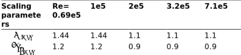
Table 4 Proposed values for Ce,max and A/Dmax
curves for different Re and surface roughness ratio k/D=2.0e-3
Scaling paramete rs
Re=
0.69e5 1e5 2e5 3.2e5 7.1e5
Ce,max 1.44 1.44 1.1 1.1 1.1
A D
� max 1.2 1.2 0.9 0.9 0.9
Step 3: Location of the peak Ce values in terms of 𝑓𝑓̂
By aligning the maximum Ce in terms of non-dimensional
frequency in the load model with the non-dimensional frequency at which the maximum response was observed in model testing at prototype scales, one can ensure that the correct dominating frequency will be predicted. There are currently two high Reynolds Free VIV model tests with the necessary response information available:
(Lie, Braaten, Szwalek, Russo, & Baarholm, Drilling riser VIV test with protorype Reynolds numbers, 2013) and (Yin, Prototypes Rn effects on riser VIV, 2015), tested both a smooth and a rough pipe mounted on springs which was restricted to pure CF motion at high Reynolds numbers and they observed that
• The smooth pipe (k/D=5x10-5) at a Reynolds number
of ~4x10⁵, had a maximum response amplitude of 0.5
diameters and occurred at a non-dimensional frequency ~0.12.
• The rough pipe (k/D=1x10-3) at a Reynolds number of
~4x10⁵, had a maximum response amplitude of 0.9
diameters and occurred at a non-dimensional frequency ~0.13
• The rough pipe (k/D=1x10-3) at a Reynolds number of
~2x10⁵, had a maximum response amplitude of 0.9
and occurred at a non-dimensional frequency ~0.18. (Vandiver & Resvanis, Improving the state of the art of high Reynolds number VIV model testin of ocean risers, 2015) tested a rough pipe mounted on springs and restricted to pure CF motion at high Reynolds and damping ratios that ranged between 0.09 and 0.27 of critical and observed that:
• For the rough pipe (k/D~2x10-3) at a Reynolds number
of ~5x10⁵ the maximum amplitude was between
~0.55-0.75 diameters, depending on the amount of damping present and repeatedly occurred at non-dimensional frequencies between 0.16-0.18
• For the rough pipe (k/D~2x10-3) at a Reynolds number
of ~4x10⁵ the maximum amplitude was between
~0.4-0.75 diameters, depending on the amount of damping present and repeatedly occurred at non-dimensional frequencies between 0.16-0.18. (Data that has yet to be published indicates that the response amplitude can approach ~0.9 diameters in this same setup as the damping ratio approaches zero.)
Clearly, there exists variability in the reported values of the non-dimensional frequency at which maximum amplitude occurs partially due to the different surface roughness and Reynolds values and partially due to the different experimental setups. Furthermore, it is important to note, that the aforementioned tests were restricted to vibration in the CF direction only and there are indications that when the pipe is allowed to vibrate freely in both the CF and IL the non-dimensional frequency at which maximum response will occur will decrease (Dahl, Hover, Triantafyllou, & Oakley, 2010).
These are still active research topics and until further experimental evidence is available at these high Reynolds values, it is recommended that the non-dimensional frequency at which the maximum Ce occurs be set to 0.18, which is at the
upper end of the range of reported values. This will result in more conservative predictions than choosing a value at the lower end of the range, because the predicted response frequency will be higher and hence the predicted stresses and damage rates will be larger (i.e. lower predicted fatigue life).
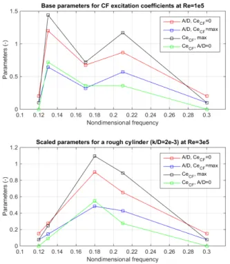
An example of the Ce model for a rough pipe (k/D=2x10^3) at
Re=1x10^5 and 3x10^5 is presented in Table 6-5. If the set of parameters presented in Figure 6-6 are used as the base excitation coefficient model, the two derived scaling parameters for a rough pipe at Re=3x10^5 are 0.76 and 0.75 respectively. The Ce,max is
scaled from 1.44 to 1.1 and the A/Dmax value is scaled from 1.2
to 0.9.
Table 5 Example of derived scaling parameters Re=1×10⁵ (base
model) Re=3×10⁵ Scaling parameter
Ce,max A D� max f̂Ce,max Ce,max A D� max f̂Ce,max 𝛄𝛄𝐂𝐂𝐞𝐞 𝛄𝛄𝐀𝐀/𝐃𝐃
1.44 1.2 0.13 1.1 0.9 0.18 0.76 0.75 Finally, it is important to note that very smooth surface pipes represent pathological cases when it comes to vortex shedding and VIV. Measured Strouhal numbers and drag coefficients for very smooth pipes show very large variability in the published literature. Furthermore, very smooth surfaced pipes mounted on springs can display extremely peculiar VIV behavior when tested in laboratory settings exhibiting both very large and very small response amplitudes on different test days due to minute testing differences that would often be considered negligible. The scaling for the very smooth pipes presented here might be of use for obtaining VIV predictions that match some of the experimentally available data but should not be used for riser design at protoype scales even if the surface finish of the riser is reported as very smooth. The reason for this is that a riser’s surface will not remain smooth for long time after it is installed due to the presence of marine growth and corrosion and it is therefore more conservative to model them as pipes with rough surfaces at these high Reynolds numbers since this approach will result in more conservative damage rate predictions.
Figure 13 Comparison of Ce parameters for a rough
pipe (k/D=2e-3) at Re=3e5 and the base parameters.
Figure 12 illustrates the peak excitation force curve for a rough pipe at a non-dimensional response frequency of 0.18. The peak excitation force curve at non-dimensional response frequency of 0.13 from the base model is also shown for comparison. (Yin, Wu, Lie, Baarholm, & Larsen, 2015)
Figure 14 Peak excitation force curve for a rough pipe
(k/D=2e-3).
Higher order response
Higher order VIV response (primarily third order) is considered to occur when the response is
• dominated by travelling waves • tension dominated
• stationary
The most important effect of higher order VIV with respect to fatigue is the increased response amplitude and hence the stress amplitude. This effect can in a simplified manner be accounted for by applying a magnification factor on the stress from response at the primary frequency per the table below.
Proposed magnification factors on stress from primary response to account for higher order response.
Structural
stiffness Description of response Stress magnification factor
Tension dominated
Stationary Travelling waves 1.4 Standing waves 1.15 Chaotic
1.05 Bending dominated
* The magnification factors are proposed based on observations in the Shell experiment and Hanøytangen experiment.
The impact of higher order harmonics on the fatigue estimate depends on the slope of the SN-curve, but it can enhance the fatigue damage by a factor of ~5 in the worst case.
A more detailed approach to account for the effect of higher order VIV is to construct higher order response modes from the primary response and calculate the associated stresses (Modarres-Sadeghi, Mukundan, Dahl, Hover, & Triantafyllou, 2010). The fatigue from this higher order VIV can then be added to the fatigue from primary response using the “dual narrow band / bi-modal spectrum” approach described in section F3, Commentary 2.2 in Appendix F of DNVGL-RP-C203, “Fatigue design of offshore steel structures”.
CONCLUSION
The main objective of this paper was to consolidate the available experimental results that describe the VIV response of cylinders at sub-critical and super-critical Reynolds numbers and propose a way this information can be used to create the excitation coefficient databases that can then be utilized by popular VIV prediction software programs.
The first part of this paper shows how an excitation coefficient database, that was based on small scale laboratory data at relatively small Reynolds numbers, can be adjusted in a manner that will allow a prediction program to accurately predict the VIV response of long elastic cylinders at sub-critical Reynolds numbers.
The second part of this paper looks at the available high Reynolds experimental data and suggests ways whereby the previously identified force coefficient database might be modified to reflect what is currently known about the VIV response of smooth and rough surfaced cylinders in the critical and super-critical Reynolds regimes.
The information included in this paper forms just a small part of a much larger document currently being prepared by DNV-GL and titled “Guideline on analysis of vortex-induced vibrations in risers and umbilicals” which includes best practices on structural modelling, current profile description, heave induced VIV, fatigue calculation and VIV suppression. This study is motivated by the desire to understand and eventually reduce the considerable variation that is often seen today in VIV predictions. The goal is to consolidated the most important information currently available in the literature and offer engineers the necessary guidance so that they can approach VIV modeling in a systematic manner.
NOTES
The work also includes best practices on • structural modelling
• current description • heave induced VIV • fatigue calculation • VIV suppression
These items are left out the current paper to reduce the scope. Note that some of the topics discussed herein are still subject of intensive research e.g. VIV in critical and super-critical flow and higher order effects. Efforts should be made to complement the data set and investigate correlation with other relevant parameters to improve the understanding.
ACKNOWLEDGMENTS
The authors are grateful to the Norwegian Deepwater Program (NDP) for support, valuable discussions, funding and permission to publish the work.