Comprehensive Identification and Spatial Mapping of
Habenular Neuronal Types Using Single-Cell RNA-Seq
The MIT Faculty has made this article openly available.
Please share
how this access benefits you. Your story matters.
Citation
Pandey, Shristi et al. “Comprehensive Identification and Spatial
Mapping of Habenular Neuronal Types Using Single-Cell RNA-Seq.”
Current biology 28 (2018): 1052-1065.e7 © 2018 The Author(s)
As Published
10.1016/J.CUB.2018.02.040
Publisher
Elsevier BV
Version
Author's final manuscript
Citable link
https://hdl.handle.net/1721.1/125056
Terms of Use
Creative Commons Attribution-NonCommercial-NoDerivs License
Comprehensive Identification and Spatial Mapping of Habenular
Neuronal Types Using Single-cell RNA-seq
Shristi Pandey1,7, Karthik Shekhar2, Aviv Regev2,3, and Alexander F. Schier1,2,4,5,6,7,8
1Department of Molecular and Cellular Biology, Harvard University, Cambridge, MA, 02138, USA 2Klarman Cell Observatory, Broad Institute of MIT and Harvard, 7 Cambridge Center, Cambridge,
MA, 02142, USA
3Howard Hughes Medical Institute and Koch Institute of Integrative Cancer Research Department
of Biology, Massachusetts Institute of Technology, Cambridge, MA, 02140 USA
4Center for Brain Science, Harvard University, 52 Oxford Street, Cambridge, MA, 02138 USA 5Biozentrum, University of Basel
6Allen Discovery Center for Cell Lineage Tracing, University of Washington, Seattle
SUMMARY
The identification of cell types and marker genes is critical for dissecting neural development and function, but the size and complexity of the brain has hindered the comprehensive discovery of cell types. We combined single-cell RNA-seq (scRNA-seq) with anatomical brain registration to create a comprehensive map of the zebrafish habenula, a conserved forebrain hub involved in pain processing and learning. Single-cell transcriptomes of ~13,000 habenular cells with 4X cellular coverage identified 18 neuronal types and dozens of marker genes. Registration of marker genes onto a reference atlas created a resource for anatomical and functional studies and enabled the mapping of active neurons onto neuronal types following aversive stimuli. Strikingly, despite brain growth and functional maturation, cell types were retained between the larval and adult habenula. This study provides a gene expression atlas to dissect habenular development and function and offers a general framework for the comprehensive characterization of other brain regions.
TOC image
7Corresponding authors. [email protected]; [email protected]; Phone: (617) 496-4835.
8Lead Contact. [email protected]; Phone: (617) 496-4835
Publisher's Disclaimer: This is a PDF file of an unedited manuscript that has been accepted for publication. As a service to our
customers we are providing this early version of the manuscript. The manuscript will undergo copyediting, typesetting, and review of the resulting proof before it is published in its final citable form. Please note that during the production process errors may be discovered which could affect the content, and all legal disclaimers that apply to the journal pertain.
AUTHOR CONTRIBUTIONS
Conceptualization, S.P., and A.F.S.; Methodology, S.P. and K.S.; Software, K.S. and S.P.; Validation S.P.; Formal analysis S.P. and K.S.; Library preparation and sequencing, S.P.; Data Curation, S.P. and K.S.; Resources, A.R. and A.F.S, Writing-Original Draft S.P., K.S., and A.F.S.; Writing-Review and Editing S.P., K.S., A.R., A.F.S; Visualization, S.P.
HHS Public Access
Author manuscript
Curr Biol
. Author manuscript; available in PMC 2019 April 02.Published in final edited form as:
Curr Biol. 2018 April 02; 28(7): 1052–1065.e7. doi:10.1016/j.cub.2018.02.040.
A
uthor Man
uscr
ipt
A
uthor Man
uscr
ipt
A
uthor Man
uscr
ipt
A
uthor Man
uscr
ipt
Pandey et al. use scRNA-seq to define more than a dozen different neuronal types in the zebrafish habenula. Cell types are retained between larva and adult.
INTRODUCTION
The study of formation and function of neural circuits relies on the ability to identify specific cell types that are defined by location, morphology, connectivity and molecular composition. Classical histological and gene expression analyses have recently been extended to single-cell technologies that enable de novo identification of cell types based on their transcriptomes [1–7]. Such studies have provided valuable resources for cataloguing cell types but are limited in their comprehensive classification by the large number and diversity of neurons in vertebrate brains. This complexity results in low sampling of rare cell types even with recent technologies that allow profiling of thousands of individual neurons in a single experiment [8, 9]. With the possible exception of a single class of interneurons in the mouse retina, we lack comprehensive catalogues of cell types in any region of the vertebrate brain [10].
One scenario in which sampling limits can be overcome is in the case of specific and conserved brain regions in animals with compact size. To test this approach, we analyzed the zebrafish habenula, a small forebrain region that is composed of approximately ~1,500 neurons at the larval stage. The habenula is a conserved structure that plays fundamental roles in vertebrate neurophysiology and behavior [11]. It receives input from a large number of brain regions, and can influence a wide range of behaviors, including sleep, pain
processing, reward learning, and fear [11–13]. Its pathophysiology has been implicated in neurological disorders such as depression, schizophrenia and addiction [14].
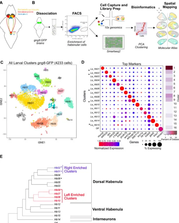
Current anatomical and molecular analysis partitions the zebrafish habenula into three major sub-regions: the nptx2a expressing dorso-lateral domain, the gpr151/pou4f1 expressing dorso-medial domain, and the aoc1 expressing ventral domain (Figure 1A). Neurons in these
A
uthor Man
uscr
ipt
A
uthor Man
uscr
ipt
A
uthor Man
uscr
ipt
A
uthor Man
uscr
ipt
domains project to distinct downstream regions in the interpedunculur nucleus (IPN) and raphe nucleus, thus mediating distinct behavioral outputs [11, 15]. These domains are also homologous to distinct domains in the mouse habenula[16]. For instance, the ventral habenula of zebrafish shares gene expression and projection patterns with the mammalian lateral habenula [17]. Furthermore, domain-specific genes are often used as genetic handles in functional studies [18–20].
It has been unclear, however, whether individual neurons in these sub-nuclei represent a single neuronal type or a mixture of multiple types. In addition, the zebrafish habenula displays a remarkable left-right (L-R) asymmetry in gene expression and functionality [21]. A number of genes such as adcyap1a, nrp1a, tac1, tac3a, slc5a7a are left-right asymmetric in the dorsal habenula [17, 22–25]. Recent studies have also shown left-right asymmetry in functional responses to light and odor in the left and right habenula, respectively [26–28]. It is also unclear if these neuronal ensembles represent transcriptionally distinct neuronal types. A comprehensive definition of habenular neuronal types is therefore needed to study its development and anatomy, and relate molecularly defined neuronal types to functional roles.
To address this challenge, we combined scRNA-seq with anatomical brain registration and created a gene expression atlas composed of more than a dozen distinct neuronal types. We find that neuronal types are anatomically organized into spatially segregated sub-regions and are stable between larval and adult stages. We show that the reference atlas enables
comparison of molecularly defined neuronal types with those defined by neural activity. Our approach constitutes a general framework for future studies aiming to comprehensively characterize other brain regions.
RESULTS
Isolation and Transcriptional Profiling of Single Larval Zebrafish Neurons
Since scRNA-seq had not been previously applied to zebrafish neurons, we devised and optimized a robust protocol for dissociation and capture of single neurons from the zebrafish brain. We found that successful experiments required gentle trituration, reduced processing time post dissociation (<30 minutes) and minimal sort pressure during fluorescence activated cell sorting (FACS) (STAR Methods). We sorted habenular cells using the gng8-GFP transgenic line [22], which selectively labels most neurons in the habenula, except for a small ventral subpopulation [23]. Heterogeneity in this subpopulation was captured using adult animals as described later.
We used two complementary scRNA-seq platforms (Figure 1B, STAR Methods): (1) Massively-parallel droplet based, 3′ end scRNA-Seq (commercial 10X Chromium platform) [29]. (2) Lower-throughput, plate-based, full-length scRNA-Seq (SMART-Seq2) [30]. We obtained data from 4,365 larval cells using droplet-based scRNA-seq (henceforth droplet dataset) sequenced at a median depth of 66,263 reads per cell, and 1,152 larval cells using SMART-seq2 (henceforth SS2 dataset), sequenced at a median depth of 1 million reads per cell. Despite the low levels of RNA in zebrafish neurons (~ 6 times less than mouse dendritic cells which are of comparable size; Figures S1A and S1B), we detected on average 1,350
A
uthor Man
uscr
ipt
A
uthor Man
uscr
ipt
A
uthor Man
uscr
ipt
A
uthor Man
uscr
ipt
(droplets) and 3,850 (SS2) genes/cell (Figures S1C, S4A). Thus, multiple scRNA-seq platforms can be effectively applied to neurons in the zebrafish brain.
Graph Clustering Identifies 15 Transcriptionally Distinct Clusters in the Larval Habenula
To identify neuronal types, we used the droplet dataset, because cell type identification was more robust with more cells sequenced at a shallow depth than few cells sequenced deeply (detailed analysis in Figure 4) [10]. We used standard computational pipelines to align the raw sequencing data to the zebrafish transcriptome and derive a gene expression matrix of 13,160 genes across 4,233 filtered cells (STAR Methods). To select highly variable genes, we used two approaches: (1) A variable gene selection method implemented in Seurat [31], and (2) an alternative approach that ranks genes based on deviation from a null statistical model built on the relationship between variation in transcript counts and mean expression per cell (STAR Methods).
We used principal component analysis (PCA) on a gene expression matrix across 1,436 variable genes and identified 36 statistically significant principal components PCs (n=36, p < 0.05). These PCs were used to build a k-nearest neighbor graph of the cells, which was then partitioned into 14 transcriptionally distinct clusters using smart local moving community detection algorithm [32] as implemented in the Seurat R package [31]. Two of these clusters held additional heterogeneity and were further partitioned using iterative clustering (Figure S1G). The resulting 16 clusters were visualized in two dimensions using t-distributed stochastic neighborhood embedding (t-SNE) (Figure 1C), and evaluated for differential gene expression to identify cluster-specific markers (Figures 1D) [10, 32, 33].
Of the 16 clusters identified in our analysis, 15 were habenular neuronal types (Hb01-Hb15) as they robustly expressed gng8 and other habenular genes (Figure S2A). We also identified a small sub-group of olfactory placode cells (Olf) that are labeled by the gng8-GFP line, based on their expression of epcam, calb2a and v2rl1 (Figure 1E) [34]. This provides an internal control and demonstrates the strength of scRNA-seq to identify contaminant types and remove them from further analysis.
To determine whether clusters corresponded to new or previously described neuronal types, we identified a host of markers for each cluster (Table S1, Figure S1L). The majority of clusters were defined by newly identified markers (Figure 1D). We also determined the relationship between these putative neuronal types using a dendrogram constructed on the variable genes across the dataset (Figure 1E). Some clusters recovered in our data comprise <1% of the dataset (Figure 1D, side bar), underscoring the advantages of oversampling cells in resolving rare types. Indeed, downsampling analysis on the droplet data suggests that we have reached saturation, but that reducing the number of cells by 20% would lead to recovery of fewer clusters (Figures S1H–S1K). These results demonstrate that the small number of neurons in larval habenula can be partitioned into 15 distinct clusters when the cells are sampled at a high frequency.
A
uthor Man
uscr
ipt
A
uthor Man
uscr
ipt
A
uthor Man
uscr
ipt
A
uthor Man
uscr
ipt
Most Previously Described Region-specific Genes are Expressed Broadly Across Multiple Neuronal Clusters
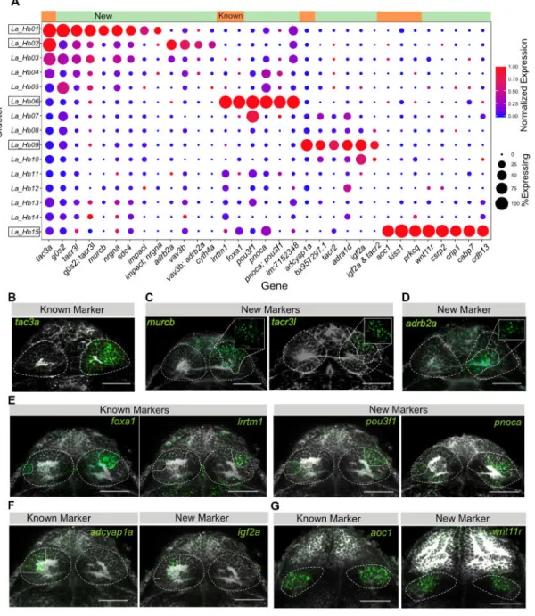
To understand how our cluster-specific markers relate to previously described habenular genes, we examined the expression patterns of these spatially localized genes among our clusters (Figures 2 and S2A). We found three major patterns.
First, some known genes show a near perfect overlap with single clusters and were also independently identified as cluster specific markers by our analysis. For example, adcyap1a, a known ‘left-only’ marker [18] is specific to cluster Hb09. Similarly, known ventral genes such as aoc1 [17, 18, 22] and kiss1 [35] are specific to cluster Hb15 (Figure 2A). For such neuronal types, we nominated a host of additional markers (e.g., Hb06 (pnoca, pou3f1), Hb09 (igf2a, adra1d, tacr2), Hb15 (csrp2, crip1, cabp7, cdh13, wnt11r)) and confirmed their spatially restricted expression patterns (Figures 2E–G).
Second, some genes that were known to mark subdomains within the dorsal habenula spanned a few clusters. For instance, tac3a, a previously described marker [25], is expressed in multiple clusters but at much higher levels in Hb01 and Hb02 (Figure 2A). Cluster specific markers for Hb01 (murcb) and Hb02 (adrb2a) seemed to subdivide the high tac3a expressing neurons in the habenula (Figures 2A–D).
Third, most genes previously reported to have regional expression patterns within the habenula were expressed across multiple clusters [17, 23–25, 35] (Figure S2A). For example, gpr151/pou4f1, which together form classic dorso-medial markers [19, 36] and nptx2a, a dorso-lateral marker [18], were expressed in majority of clusters, albeit at different levels (Figure S2A). We detected higher expression of nptx2a in the left habenular clusters (Figure S2A), confirming the previously observed over-representation of lateral identity in the left habenula [24]. We validated the overlap of these classic markers with multiple clusters by RNA-FISH (Figure S2B), demonstrating that individual genes reported to be spatially restricted could span multiple neuronal subtypes.
Among our newly identified markers, we found: 1) markers that are expressed exclusively in the cluster of interest (‘digital’), 2) markers that display 2-3 fold enrichment in the cluster of interest (‘analog’). To compare the specificity of marker genes, we computed their area under the precision recall curve (AUCPR) as a quantitative measure of “cluster-specificity” (See STAR Methods). Digital markers such as aoc1 displayed AUCPR values greater than 0.8 (Figure S2C) whereas analog markers such as tubb5 exhibited lower AUCPR values (0.55 – 0.7). We found that considering pairs of analog markers affords higher specificity in defining a cluster. For instance, pou3f1 and pnoca together localize Hb06 better than each does individually (Figure 2E). Therefore, we only used single markers with AUCPR > 0.7 to spatially localize clusters of interest.
Taken together, these results provide novel analog and digital markers for the five clusters that were readily defined by expression of known genes and describe their in vivo spatial localization. Strikingly, the majority of previously described habenular genes are broadly expressed over multiple clusters, limiting their utility as markers for transcriptionally distinct neuronal types.
A
uthor Man
uscr
ipt
A
uthor Man
uscr
ipt
A
uthor Man
uscr
ipt
A
uthor Man
uscr
ipt
Analysis and Validation of Previously Uncharacterized Habenular Neuronal Types
The remaining 10 of 15 clusters expressed marker genes that to our knowledge have not been previously described in the zebrafish habenula. We hypothesized that these clusters corresponded to potentially novel neuronal subtypes and performed RNA-FISH with cluster-specific markers to validate them and determine their spatial localization (Figure 3). We also utilized the gene expression dendrogram (Figure 1E) to relate them to ‘known’ neuronal types described earlier. Based on spatial localization, we found three major categories of neuronal subtypes.
First, we identified three new ‘left-enriched’ clusters of neurons – Hb07(pcdh7b+) and Hb08(wnt7aa+), Hb10(ppp1r1c+) – all of which were closely related to one another and to ‘left-only’ neuronal type Hb09 (adcyap1a+) (Figure 1E). All of these clusters also expressed another known ‘left-only’ marker, nrp1a (Figure S2A) [24]. Hb08 (wnt7aa+) and Hb10 (ppp1r1c+) neurons were localized more dorsally in the left habenula than Hb07 (pcdh7b+) (Figure 3A).
Second, we identified three posterior L-R symmetric habenular neuronal types (Figure 3B). Dorsally located Hb04 was characterized by the expression of cbln2b, a less studied member of the cerebellin genes, some of which are important for synaptic plasticity [37]. Ventrally located pyya+ neurons were subdivided into Hb11 (cpne4a+) and Hb12 (htr1aa+).
Corresponding to their low proportion by scRNA-seq, RNA-FISH showed that Hb11 and Hb12 are both rare, composed of 4-6 neurons in vivo.
Third, we found four rare neuronal types, each comprising less than 5% of the cells in our dataset. Hb03(spx+) and Hb05(c1ql4b+) form rare populations that seem to be distributed in a non-regionalized manner (Figures 3C, upper panels). Hb13 is a cluster of immature neurons in the medial ventral habenula and lining the ventricular zone, characterized by the expression of tubb5 and a host of ribosomal proteins (Figure 3C) [38]. Rarest among these four types were GABAergic neurons in the dorsal habenula (Figures 1D and 3C)
characterized by the expression of gad1b, gad2 and the GABA transporter slc32a1 and corresponding to 2-3 neurons in vivo.
Together, these results provide validation and spatial localization for the 10 novel neuronal types identified by our single-cell analysis and demonstrate a general trend for
regionalization of neuronal types within the habenula. Moreover, transcriptional proximity was reflected by spatial proximity in vivo, suggesting that developmental patterning of molecularly related neuronal types occurs in a spatially restricted manner.
Computational Image Registration Generates a Spatial Map of Neuronal Types in the Habenula
To explore the localization of neuronal types in relation to one another, we created a consolidated spatial map of neuronal type specific markers in the habenula (Figure 3D, 3E and Movie S1). We used computational image registration to morph RNA-FISH signals across multiple zebrafish larvae onto a single reference based on the total ERK (tERK) antibody stain [39–41] (Figure S3A, S3B) resulting in a reference spatial map of the habenula (Movie S1).
A
uthor Man
uscr
ipt
A
uthor Man
uscr
ipt
A
uthor Man
uscr
ipt
A
uthor Man
uscr
ipt
Our map demonstrates that a majority of habenular types were regionalized either along the dorso-ventral, medio-lateral or left-right axis, suggesting that habenular types can be defined not only by their transcriptomes but also by distinct spatial positions (Figure 3E, Movie S1). Eleven types were located more dorsally in the habenula; 8 of them seem to be regionalized: Hb01/Hb02 were right enriched or exclusive, Hb07/Hb08/Hb09/Hb10 were left-enriched or exclusive, Hb04 and Hb06 was L-R symmetric in the dorsal habenula. Four types were located more ventrally, of which Hb11 and Hb12 were posterior ventral populations, Hb15 occupied a large portion of the ventral habenula and Hb13 formed a germinal zone along the medial region of the ventral habenula. In summary, our fluorescent in situ atlas provides the first spatial map of the 15 known and novel neuronal types in the zebrafish habenula.
Neuronal Types in the Larval Habenula and Their Molecular Signatures are Robustly Reproduced in Full-Length, Deeply Sequenced Libraries
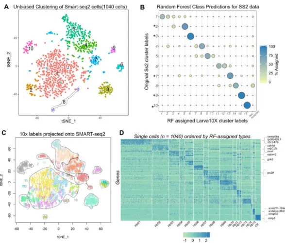
Because zebrafish neurons contain less RNA than other cell types – including of comparable size – analyzed using scRNA-seq (Figures S1A and S1B) [10, 42], we asked if we could derive a better classification by sequencing these neurons at a greater depth. To explore this possibility, we prepared 1,152 SMART-seq2 (SS2) libraries using cells sorted from the gng8-GFP transgenic line [30], and sequenced them at a median depth of 1 million reads per cell (~25 fold deeper than the droplet data; Figure S4A and S4B), resulting in 3,850 genes/ cell, (~3 fold more than the droplet data).
An independent clustering of 1,040 quality-filtered SS2 cells revealed only 10 clusters (Figure 4A), fewer than the droplet data. We hypothesized that the lower number of cells in SS2 dataset led to merging of closely related clusters. To evaluate the correspondence between droplet and SS2 clusters, we trained a multiclass random forest classifier (RF) on the cluster labels of the droplet dataset (Figure S4I) and used it to map all the SS2 cells onto droplet-based labels [10, 43]. We observed that 5 out of 10 SS2 clusters mapped 1:1 with single droplet clusters (Figure 4B). Each of the four remaining SS2 clusters mapped to multiple (typically 2-3) droplet clusters (Figure 4B). By labeling each cell on the tSNE plot with RF assigned cluster labels, we observed additional sub-structure in the merged SS2 clusters that was masked in unsupervised clustering (Figure 4C). This co-clustering occurs in cases where clusters are closely related (Figure 1E) but not highly represented in the dataset (eg: Hb05-Hb03, Hb02-Hb01-Hb04, Hb07-Hb08). These results are also consistent with the recovery of fewer and less pure clusters in the downsampled droplet dataset (Figure S1H–S1K).
Next, we asked if the higher number of genes/cell identified in SS2 data enabled the identification of novel cluster-specific markers. To this end, we examined genes that were robustly detected in the SS2 data but not in droplet data (Figures S4J–S4K and Figure S4L, red), but found that they were expressed across multiple clusters and were uninformative for cell type classification (Figure S4M, STAR Methods). Using differential gene expression analysis on the RF-assigned cell labels, we identified a small number of novel cluster-specific markers that were not identified in droplet dataset (Figure 4D, highlighted along heatmap).
A
uthor Man
uscr
ipt
A
uthor Man
uscr
ipt
A
uthor Man
uscr
ipt
A
uthor Man
uscr
ipt
Taken together, these results demonstrate a remarkable consistency of types and markers discovered by two different scRNA-seq platforms. Also, consistent with earlier work [10], these results show that cell type identification is best served by distributing a given number of reads over a large number of cells.
Neurons in the Adult Habenula Retain the Molecular Identity of Larval Types
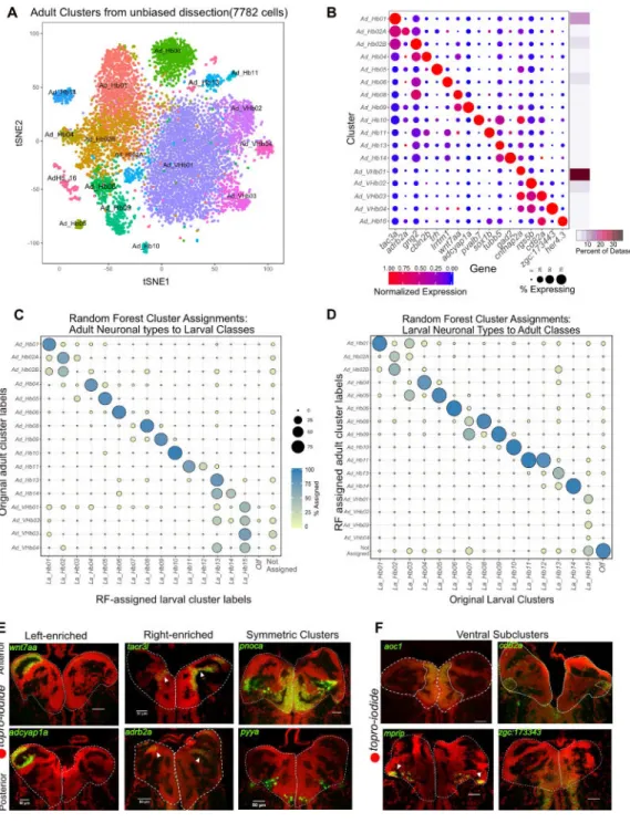
The habenula undergoes significant growth, morphogenesis and functional maturation from developing larvae to mature adults (Figure S5I, left). For example, several behaviors mediated by habenular neuronal subpopulations such as aggression are only displayed by adult fish, and the number of neurons increases dramatically between larva and adult [18, 19]. Furthermore, the larval dataset was generated with a transgenic line with FACS and may have missed rare populations not labeled by the gng8-GFP. To assess the conservation and retention of neuronal types from larva to adult fish (1-year old) and to capture cells that were not labeled by the transgenic line, we dissected whole adult habenulae and performed droplet scRNA-seq (STAR Methods). Post quality filtering, we obtained 7,782 single cell profiles at a median depth of ~96,000 reads and 709 genes per cell (Figure S5A, S5B). Using the same clustering approach, we detected 17 clusters and enriched markers (Figures 5A and 5B) and labeled them post-hoc by comparison to the larval clusters (below). To systematically compare the clusters between larva and adult, we used a random forest model trained on either dataset to map gene expression signatures between the two datasets (Figure 5C (trained on larva) and Figure 5D (trained on adult)). Since the larval dataset was generated by cellular sorting based on the gng8-GFP line, we restricted our analysis to the high gng8+ cells in the adult dataset. Using the RF model, we then classified each high gng8+ adult cell (Figure S5F) into one of the larval cluster labels (Figure 5C). Surprisingly, we found that 9 out of the 16 adult habenular clusters mapped 1:1 to single larval habenular clusters (Figure 5C). The left-right spatial organization of some clusters was also roughly preserved (Figure 5E).
We also found that some larval clusters map to multiple adult clusters. For instance, La_Hb02 (La = Larval) split into Ad_Hb02A and Ad_Hb02B (Ad = Adult). Upon interrogating the differences between Ad_Hb02A and Ad_Hb02B further, we found that certain genes such as nebl are selectively expressed in Ad_Hb02B (Figure S5G) whereas others such as rac2 are in Ad_Hb02A. Furthermore, larval ventral cluster, La_Hb15 mapped to multiple adult types, all of which are ventral (Ad_VHb01-04) as found by RNA-FISH for differentially expressed markers cntnap2a, mprip, cd82a, and zgc:173443 (Figure 5F). The spatial localization of these ventral clusters was found to be consistent with previously described [17] morphogenetic changes that occur in the habenula between larval and adult stages (Figure S5I).
This multi-mapping among ventral clusters was likely caused by incomplete labeling of ventral habenula by the gng8-GFP line, which was used to capture cells in larval dataset. In particular, in situ hybridization revealed that two of the adult ventral type markers were expressed in a spatially restricted pattern in the larval ventral habenula (Figure S5D). We also found a small population of neuronal progenitors (her4+, fabp7a+, mdka+) in the medial
A
uthor Man
uscr
ipt
A
uthor Man
uscr
ipt
A
uthor Man
uscr
ipt
A
uthor Man
uscr
ipt
ventral habenula (Figures 5B and S5E), in a similar location as the immature tubb5+ (Figure 3D) neurons in the adult dataset.
Taken together, these results demonstrate that despite significant growth and functional maturation between larvae and adults, a substantial proportion of neuronal types in the habenula remain largely constant.
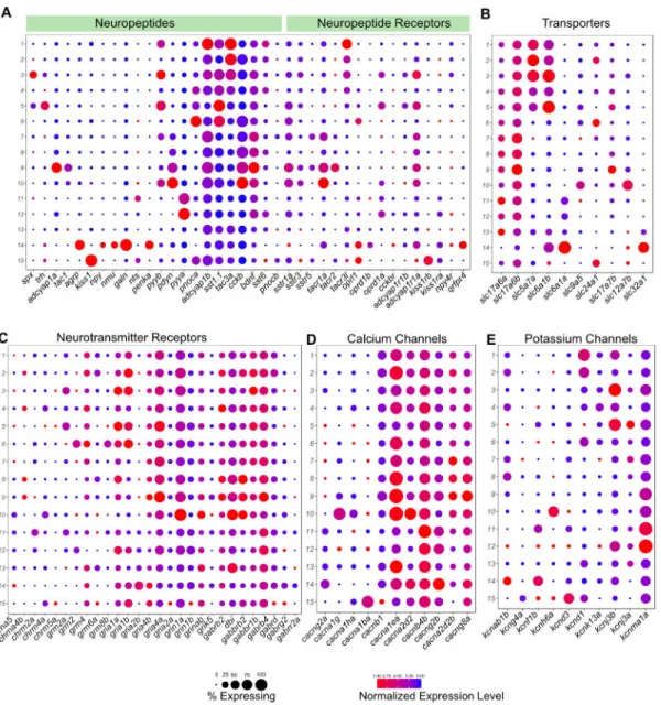
Neuropeptidergic Signaling, Neurotransmission and Neuroexcitability Among Habenular Neuronal Types is Highly Diverse
Previous studies have used ISH or immunostaining to assess the expression of various neuropeptidergic and neurotransmitter genes in the habenula [22, 23] but a comprehensive expression profile of these genes is not available. Using the scRNA-seq dataset, we assessed the expression profiles of these genes among the different neuronal types in the larval (Figure 6) and adult (Figure S6) habenula.
We found that a large number of neuropeptides are specific to a small number of neuronal types (Figures 6A and S6A). For example, spx, trh, adcyap1a, tac1, agrp, kiss1, npy, galn, penka were all expressed in only one habenular type each, whereas pyya, pyyb, pdyn, pnoca, sst1.1, tac3a, cckb were enriched in 2-4 neuronal types. In addition, co-expression of multiple neuropeptides was a common feature among habenular neuronal types. For instance, spx, which acts as a satiety factor and pyyb, which has been implicated to be an anorexigenic factor, were co-expressed in the homologous clusters in both larvae and adults respectively [44]. Conversely, we examined the expression profile of all detectable
neuropeptide receptors. In some cases, the same neuronal type produces a neuropeptidergic signal and expresses its cognate receptor, suggesting autocrine signaling. For instance, kiss1 and its receptors kiss1rb and kiss1ra are co-expressed in ventral habenular clusters (Figures 6A and S6A).
Next, we analyzed the expression of genes essential to signal transduction in neurons. As previously observed [45], a large proportion of habenular neurons are glutamatergic, as reflected in the broad expression of glutamate transporters slc17a6a and slc17a6b (Figure 6B). However, the habenula also contains a small population of GABAergic neurons (Figure 6B). Hb01 through Hb05 are also cholinergic and express the choline transporter slc5a7a (Figure 6B). Cholinergic transmission was largely absent in left-enriched neuronal types consistent with previous studies [22]. Similarly, some neurotransmitter receptor subunits such as grm8b, grm2, gria2b are enriched in one or a few clusters (Figure 6C). Calcium channels such as cacng2a, cacna1g, cacna1ba are also expressed in a type specific manner, as are potassium channel subunits such as kcnab1b, kcnf1b, kcnh6a, kcnd3 (Figure 6D and E). We found a similar distribution of these functionally relevant genes in the adult habenula (Figure S6A–F). Collectively, our data shows that despite being a small region, the habenula shows a remarkable diversity in expression of genes that directly influence the functional and electrophysiological properties of individual neurons.
Functional Assignment onto Molecularly Defined Neuronal Types
Finally, we began to explore if and how functional responses of the habenula are distributed among these transcriptionally distinct neuronal types. To this end, we performed a
proof-of-A
uthor Man
uscr
ipt
A
uthor Man
uscr
ipt
A
uthor Man
uscr
ipt
A
uthor Man
uscr
ipt
principle experiment to determine if we could use neuronal type specific markers and the reference habenular atlas (Figure 3E and Movie S1) to map responses to specific stimuli among the molecularly defined neuronal types. We exposed fish to electric shocks, and assessed upregulation of the immediate early marker gene cfos in specific neuronal types. We observed localized upregulation of cfos expression in specific sub-regions within the habenula in shocked animals (Figure 7A). We registered the cfos RNA-FISH signals onto our reference habenular map, and detected overlap within the domains of expression of left habenular Hb09 (adcyap1a+), posterior habenular Hb04 (cbln2b+) and largely within the ventrolateral population (mprip+) (Figure S7A, Figures 7A, 7B). Double in situ
hybridization for mprip and cfos showed a regional overlap between the mprip+ and cfos+ cells in both larva (Figure 7C) and adult (Figure 7D, Movie S2). Together, these results show that neuronal ensembles in the ventrolateral habenula comprise a large proportion of cells responsive to aversive electric shocks and demonstrate the utility of the habenular atlas to link functional responses to molecularly defined neuronal types.
DISCUSSION
We used two scRNA-seq platforms, integrative computational analysis, and brain
registration to build and validate a comprehensive atlas of neuronal types in the larval and adult zebrafish habenula. Our study provides six main advances. First, we devised a robust protocol for the dissociation and capture of single neurons from the zebrafish brain. Second, we found that comprehensive identification of neuronal types by scRNA-seq can be achieved by high cell-sampling coverage of a small brain region. Third, we discovered thirteen new neuronal types and identified fine-grained spatial subdivisions in the habenula. Fourth, we discovered dozens of new marker genes that define habenular neuronal types. Fifth, we found that diverse neuronal types are largely retained from larva to adult. Sixth, we showed that the reference atlas enables comparison of molecularly defined neuronal types with those defined by neural activity. Taken together, our study creates a resource for future studies on habenular development and function and provides a technological framework for the characterization of other brain regions.
Single-Cell Analysis of the Zebrafish Brain
Although scRNA-seq is now well-established, applying it to zebrafish neurons presents certain technical challenges. Our work establishes critical conditions for future scRNA-seq in the zebrafish brain. We provide a robust dissociation and sorting based cell capture protocol for zebrafish neurons (STAR Methods), which were found to have comparatively less RNA than other cell types. Consistent with previous studies, we also found that transcriptional signatures required to classify cell types can be identified by low coverage RNA-seq [10]. Therefore, most of the additional genes detected in the deeper SMART-seq2 dataset were uninformative for cell type classification (Figure S4M).
Comprehensive Cell Type Identification and Spatial Mapping in the Habenula Facilitates Functional Studies
Based on scRNA-seq on larva and adults, we found that the habenula is composed of at least 18 distinct neuronal subsets. While larval ventral heterogeneity needs to be explored genome
A
uthor Man
uscr
ipt
A
uthor Man
uscr
ipt
A
uthor Man
uscr
ipt
A
uthor Man
uscr
ipt
wide using RNA-seq approaches, our two-time point scRNA-seq and in situ analysis has allowed us to describe the majority of the neuronal types in the habenula. For each of these neuronal types, we found dozens of novel molecular markers. Whole brain in situ
hybridization showed that some of these markers are exclusively expressed within habenular neuronal subsets, making them good candidates for generating reporter lines (Figure S3C). We also used RNA-FISH and image registration to spatially localize neuronal types, a key step in linking molecular profiles to physiological and behavioral features. We found that 15 neuronal subsets are highly regionalized to habenular sub-regions (Figures 3L, 5F). This arrangement is similar to regionalization observed in the hippocampus [46] but in contrast to the organization in the retina where different cell types are intermixed within the same spatial location [47].
Furthermore, we found that previously demarcated anatomical sub-regions, dHbM (pou4f1+, gpr151+), dHbL (nptx2a+) and vHb (aoc1+) harbor multiple transcriptionally distinct neuronal subsets. Previous studies have shown that these distinct sub-regions send efferent projections to distinct anatomically separated sub-regions of the downstream
interpeduncular nucleus (IPN) and raphe nucleus [15]. Our study raises the possibility of a finer topography of efferent projections of transcriptionally distinct neuronal subsets into finer sub-regions of downstream targets.
We also found a large diversity of neuropeptidergic genes in the habenula, which may shed light into its unexplored functional roles. For instance, a number of peptides that are involved in food intake regulation such as cckb, pyya, pyyb, and spx are shown to be robustly expressed in certain sub-clusters of habenular cells, indicating that the
corresponding neuronal types may be important for regulating food intake. Furthermore, a subset of the pyya neurons are positive for htr1aa, a serotonin receptor whose expression is known to be affected by anorexigenic drugs [48].
Therefore, our comprehensive list of neuronal types along with dozens of marker genes and their spatial map will be a valuable resource for the study of habenular development and function in normal and pathophysiological conditions.
Neurons in the Adult Habenula Retain the Molecular Identity of Larval Types
Cell type identification should distinguish between stable cell types and transient cell states as transcriptional cascades in individual neurons may change in response to a variety of different stimuli such as neural activity, neuropeptides, hormones or developmental signals. Our two time-point study design enabled us to observe the remarkable congruence of habenular subtypes between the developing 10-day old larval and the adult brain, suggesting that these signatures represent stable molecular identities. We also found that the localization of neuronal types in the adult habenula is consistent with the complex morphogenetic changes in the habenula between larva and adult wherein the ventral cells migrate inward from lateral to medial positions (Figure S5H, S5I) [17].
A number of habenula-dependent behaviors such as fear responses and aggression arise later in development in juvenile or adult zebrafish [18, 19, 49]. In the absence of major changes in
A
uthor Man
uscr
ipt
A
uthor Man
uscr
ipt
A
uthor Man
uscr
ipt
A
uthor Man
uscr
ipt
molecular cell type diversity, what circuit mechanisms account for alterations in behavioral capacities during development? An attractive hypothesis is that habenular input-output relationships change between the two time-points. For example, habenular outputs may diverge into more downstream regions to mediate a diverse set of behaviors in adults. A detailed investigation of the development of habenular inputs and outputs will be required to address this question.
Mapping the Transcriptionally Defined Neuronal Types to Functionally Distinct Types
While cell type classification is essential for understanding the form and function of neural circuits, an important future goal is to relate such molecularly defined neuronal types to functionally defined types [2]. In many brain regions, it is not clear whether distinct, transcriptionally defined sub-populations form functionally distinct motifs as well. Our work suggests that the habenula contains discrete, spatially and transcriptionally segregated functional ensembles. In particular, our cfos data suggest that habenular
responses to aversive stimuli are restricted to a few molecularly defined subsets (Figure S7), including those identified by a recent study describing the role of dorsal left habenula in recovery from electric shocks [50]. The newly identified mprip+ cells in the ventrolateral habenula merit further investigation as they co-express neurotensin, an endogenous peptide that has been emerging to have a role in stress-induced anxiety and learning (Figure S6A) [51, 52]. Similarly, our spatial map suggests that the left-exclusive neuronal subsets Hb08 (wnt7aa+) and Hb09 (adcyap1a+) form light responsive ensembles, found to be lateralized in the left habenula in previous studies [26] (Figure 3E, schematic). A number of other calcium imaging studies have described spontaneous and stimulus evoked activity maps in the habenula [27, 53]. Interfacing such functional maps to our molecular map using emerging techniques such as MultiMAP [54] will allow a systematic correlation of molecular profiles with functional properties. Our cell type catalogue and gene expression atlas provide the foundation for future studies to address the relationship between habenula functions and molecular identities.
Pipeline for Comprehensive Identification of Cell Types in Other Brain Regions
The comprehensive classification of neural types is limited by the large number and diversity of cells in vertebrate brains. For example, previous scRNA-seq studies have sampled a small percent of cells to infer heterogeneity in large regions [4, 6, 55, 56]. Our study shows that such limitations can be overcome by scRNA-seq from predefined small sub-regions at high cellular coverage. The larval zebrafish brain contains fewer than 200,000 neurons, putting its comprehensive molecular classification within reach of current technologies and creating a blueprint for cell type diversity in the vertebrate brain.
STAR METHODS
CONTACT FOR REAGENT AND RESOURCE SHARING
Further information and requests for resources and reagents should be directed to and will be fulfilled by the Lead Contact, Alexander F. Schier ([email protected]).
A
uthor Man
uscr
ipt
A
uthor Man
uscr
ipt
A
uthor Man
uscr
ipt
A
uthor Man
uscr
ipt
EXPERIMENTAL MODEL AND SUBJECT DETAILS
Zebrafish—Larvae and adult fish were maintained on 14 hours: 10 hours light: dark cycle at 28°C. All protocols and procedures involving zebrafish were approved by the Harvard University/Faculty of Arts & Sciences Standing Committee on the Use of Animals in Research and Teaching (IACUC; Protocol #25-08). Wildtype zebrafish from the TLAB strain were used. 10 days post fertilization (dpf) larval and ~1-year old adult male and female zebrafish were used across different experiments. Animals were anesthetized in 0.2% tricaine and rapidly euthanized by immersion in ice water for 5 minutes before dissection. RNA-seq experiments were performed with the transgenic lines: Tg(gng8:nfsB-CAAX-GFP) and Tg(gng8: GAL4 X UAS: mCherry) in larval and adult stages.
METHOD DETAILS
Cell Isolation and RNA-Seq
Isolation of cells for SMART-seq2: 10 dpf larval heads were dissected in Neurobasal (ThermoFisher Scientific 21103049) supplemented with 1x B-27 (ThermoFisher Scientific 17504044), and promptly dissociated using the Papain Dissociation Kit (LK003150) with following modifications. Larval heads were incubated in 20 units/mL papain for 25 minutes at 37°C. The cells were dissociated by gentle trituration 20 times and spun at 300xg for 5 minutes. The cells were resuspended in 1.1 mg/mL papain inhibitor in Earle’s Balanced Salt Solution (EBSS). The resulting cell suspension was passed through 20 μm cell strainer and placed on ice. Two viability indicators (calcein blue, a live stain (ThermoFisher Scientific C1429) and ethidium homodimer, a dead cell stain (ThermoFisher Scientific E1169)) were added at a concentration of 0.01mg/mL. If the viability of cells was greater than 85% as measured by calcein blue staining, the cells were immediately sorted directly into a 96-well plate with 5μL of lysis buffer comprised of Buffer TCL (QIAGEN 1031576) plus 1% 2-mercaptoethanol (Sigma 63689). All samples were immediately frozen in dry ice and stored at −80°C until further processing.
SMART-seq2 library preparation: For preparation of SMART-seq2 libraries, the plates containing single-cell lysates were thawed on ice and purified with 2.2X RNAClean SPRI beads (Beckman Coulter Genomics) without elution. The beads were then air-dried and processed promptly for cDNA synthesis. SMART-seq2 was performed using the published protocol [30] with minor modifications [10]. We performed 22 cycles of PCR for cDNA amplification. The resulting cDNA was eluted in 10μL of TE buffer. We used 1.25 ng of cDNA from each cell and one fourth of the standard Illumina Nextera XT reaction volume in tagmentation, and final PCR amplification steps. We pooled 384 single-cell libraries from gng8-GFP line in each batch and sequenced 50x25 paired end reads using a single kit on the Illumina NextSeq500 instrument.
Cell isolation and library preparation for Droplet scRNA-seq: 10dpf larval heads from 25 gng8-GFP fish were dissected, and cells were dissociated as described previously. After reconstitution of cells with papain inhibitor, the cells were spun again at 300xg for 5 minutes and washed with 1X Phosphate Buffered Saline (PBS). Viability indicators were added and roughly 6000-8000 cells were immediately sorted into 20μL of PBS to a final concentration
A
uthor Man
uscr
ipt
A
uthor Man
uscr
ipt
A
uthor Man
uscr
ipt
A
uthor Man
uscr
ipt
of cells 300 cells/μL. The sorting was performed with a MoFlo Astrios (Beckman Coulter) with highly reduced sort pressure at 20psi. This was found to be a critical step as higher sorting pressure led to high cell death post sorting. The resulting single cell suspension was promptly loaded on the 10X Chromium system [57]. The sorted cells were not kept on ice for longer than 10 minutes because the viability post cell sorting, as measured by trypan blue staining, was found to drop over time.
For experiments with adult animals, six adult habenulae were directly dissected out of the brain based on the expression of gng8-GFP marker. The resulting tissue was then dissociated in 1mL of 20 units/mL papain for 15 minutes at 37°C. The habenular cells were dissociated by trituration, spun at 300xg for 5 minutes and resuspended in 1mL 1.1mg/mL papain inhibitor solution. The resulting cells were then washed in 1x PBS + 200mg/mL Bovine Serum Albumin (BSA) (NEB, B9000S) once and filtered through a 20 μm cell strainer. The cells were then resuspended in 50μL PBS + 200μg/mL BSA and counted on a
hemocytometer. Viability was assessed by using a trypan blue staining and cells were loaded onto the 10X Chromium system at a concentration of ~300 cells/μL after ensuring that the cell viability in the suspension was greater than 80%. 10X libraries were prepared as per the manufacturer’s instructions [57].
Imaging Methods
Probe synthesis for RNA in situ hybridization: Fragments of the following genes were amplified using Phusion Hi-Fidelity polymerase (New England Biolabs, M0530L) with the primers listed in Table S3. The Polymerase Chain Reaction (PCR)-amplified fragments were then cloned into pSC-A plasmid using Strataclone PCR Cloning Kit (Agilent, 240205), and used to transform the Strataclone competent cells. The transformed cells were plated overnight on Luria-Bertani (LB) agar plates. Colonies were selected by colony-PCR, cultured, mini-prepped and sent for sequencing. The resulting plasmids were then restricted with the appropriate restriction enzyme (Table S3), and purified using PCR-clean up kit (Omega Cycle Pure Kit). The linearized vector was then used as a template to synthesize digoxigenin- or fluorescein-labeled RNA probes using the RNA labeling kit (Roche). The transcription reactions were purified using Total RNA clean up kit (Omega, R6834), and the resulting RNA was quantified using Nanodrop and assessed on an agarose gel. The final product was then normalized to a concentration 50ng/μL in HM+ buffer (50% formamide, 5X Saline Sodium Citrate (SSC) buffer, 5 mgmL−1 torula RNA, 50 μgmL−1 heparin, 0.1% Tween 20) and stored at −20°C until further use.
Fluorescent in situ hybridization: Fluorescent RNA in situ hybridizations were performed as previously described [58]. Zebrafish larvae were grown until 10dpf and were fixed in 4% formaldehyde (Sigma-Aldrich) in PBS at 4°C overnight. Post fixation, the larvae were rinsed three times in PBST (PBS with 0.1% Tween 20), and subsequently dehydrated in increasing concentrations of methanol (10 minutes each 25% methanol: 75%PBST, 50% methanol: 50% PBST, 75% methanol: 25% PBST and two times 100% methanol). Dehydrated larvae were then stored at −20°C at least overnight. Larvae were rehydrated with decreasing concentrations of methanol (10 minutes each, 75% methanol: 25% PBST, 50% methanol: 50% PBST, 25% methanol: 75% PBST, four times for 10 minutes PBST). They were
A
uthor Man
uscr
ipt
A
uthor Man
uscr
ipt
A
uthor Man
uscr
ipt
A
uthor Man
uscr
ipt
digested in Proteinase K (10 μg/mL) for 1 hour and immediately fixed in 4% formaldehyde to stop digestion (20 minutes). Larvae were then pre-hybridized in Hybridization Mix (HM) + buffer (50% formamide, 5× SSC buffer, 5 mg/mL torula RNA, 50 μg/mL heparin, 0.1% Tween 20) at 65°C for 2 hours. Hybridization reactions with the RNA probes were carried out in HM+ (with digoxigenin-labeled antisense probes for single in situ hybridizations and digoxigenin- or fluorescein-labeled antisense probes for double in situ hybridizations) overnight at 65°C. Probes were normalized to a concentration of 3.33ng/μL and denatured at 70°C for 10 minutes before hybridization. Sense probe controls were performed alongside the antisense probes.
The next day, larvae were washed several times at 65°C (20 minutes in hybridization mix, 20 minutes in 75% formamide: 25% 2xSSCT (2XSSC with 0.1% Tween20), 20 minutes in 50% formamide: 50% SSCT, 20 minutes in 25% formamide: 75% SSCT, twice for 20 minutes in 2x SSCT, thrice for 30 min in 0.2x SSCT. The larvae were then washed twice in TNT (100mM Tris-HCl, pH 7.5, 150mM NaCl, 0.5% Tween 20) at room temperature. The larvae were subsequently blocked in 1% Blocking Reagent in TNT (TNTB) for at least 1 hour and incubated with a peroxidase-conjugated anti-digoxigenin-POD antibody (1:400 dilution in TNTB) at 4°C overnight with gentle agitation (Anti-Digoxigenin-POD Fab Fragments, Roche 11 207 733 910).
The following morning, the antibody was removed and larvae washed in TNT (8 times for 15 minutes each). After the washes, the larvae were stained per the TSA kit instructions for 1 hour in darkness without agitation (Perkin Elmer TSA Plus Cyanine 3 System,
NEL744001KT). The larvae were then washed in TNT three times, 5 minutes each. For single in situs, a subsequent immunostaining for anti-total-Erk (Cell Signaling, 9102) was performed to use as an anatomical reference and signal for brain registration across multiple fish.
For double in situs, after the first staining reaction, the first antibody was removed by treating the larvae in 1% hydrogen peroxide for 20 minutes without agitation. The larvae were then incubated overnight with anti-fluorescein-HRP antibody (Anti-Fluorescein- POD Fab Fragments, Roche 11 426 356 910), diluted in 1:400 in blocking buffer at 4C with gentle agitation.
The following morning, the antiserum was removed and discarded, and excess antibody was removed by rinsing the embryos 8×15 minutes in TNT buffer. They were then subsequently stained by incubating in 100μL of Cy3 tyramide reagent diluted in 1:25 in amplification diluent (Perkin Elmer TSA PLUS Cyanine 3 System, NEL744991KT) for an hour without agitation. The embryos were then washed in 8X15 minutes in PBST and subsequently stained with anti-total-erk antibody for anatomical reference.
Fluorescent RNA in situ hybridization in adult zebrafish: Adult fish brains were dissected in ice-cold PBS and fixed overnight in 4% paraformaldehyde (PFA). Fluorescent RNA in situ hybridization in adult dissected brains was performed with the same protocol as outlined above with the following changes. Brains were digested in Proteinase K (20ug/mL) for 35 minutes. Following probe hybridization, antibody incubation and tyramide signal
A
uthor Man
uscr
ipt
A
uthor Man
uscr
ipt
A
uthor Man
uscr
ipt
A
uthor Man
uscr
ipt
amplification, the brains were mounted in 3% low-melt (LM) agarose and sliced into 50 micron sections using the vibratome. The resulting slices were stained with TOPRO3 (1:5000) or Sytox green (1:30,000) for nuclear staining and imaged using a Zeiss inverted Confocal microscope with a 20X air objective and a 63X oil dipping objective.
Imaging and Image Registration—The larvae were washed three in PBST, mounted in 2% LM agarose and imaged with an upright Confocal Zeiss LSM 880 with a water dipping 20× objective.
Whole Habenula Registration: Image registration across multiple habenulae was performed with CMTK (http://www.nitrc.org/projects/cmtk/) with command string (T 32 -awr 010203 -X 52 -G 80 -R 3 -A ‘–accuracy 0.8’ -W ‘–accuracy 1.6’). Template habenula was a 10dpf nacre (mitfaa −/−) larvae that underwent RNA-FISH and immunostaining with anti-total-erk. All RNA-FISH images were subsequently registered to the same reference using cmtk [39–41]. All registered images were compared to the original in situ images to screen out unnatural morphing artifacts. The best registered images were chosen manually and used for generating reference habenula (Movie S1)
Whole Brain Registrations—Whole brain registrations were performed in a similar manner by choosing a reference whole brain image from a larva that underwent RNA-FISH and immunostaining with anti-total-erk. However, subsequent registrations were performed using Advanced Normalization Tools ANTs [59] with the following parameters:
antsRegistration -d 3 –float 1 -o [fish1_,fish1_Warped.nii.gz] –interpolation
WelchWindowedSinc –use-histogram-matching 0 -r [Ref1.nii,fish1- 01.nii.gz,1] -t rigid[0.1] -m MI[Ref1.nii,fish1-01.nii.gz,1,32, Regular, 0.25] -c [200×200×200×0,1e-8,10] –shrink-factors 12×8×4×2 –smoothing-sigmas 4×3×2×1vox -t Affine[0.1] -m MI[ref/terk-ref.nii,fish1-01.nii.gz,1,32, Regular,0.25] -c [200×200×200×0,1e-8,10] –shrink-factors 12×8×4×2 –smoothingsigmas 4×3×2×1vox -t SyN[0.1,6,0] -m
CC[ref/terk-ref.nii,fish1-01.nii.gz,1,2] -c [200×200×200×200×10,1e-7,10] –shrink-factors 12×8×4×2×1 –smoothingsigmas 4×3×2×1×0vox.
Due to the high computation time required for these analyses, registrations were parallelized using Slurm-based bash scripts.
Image visualization—A non-linear gamma filter (ImageJ (Math; Gamma = 0.3)) was applied to the total-Erk channel in some images presented in the main text to aid visualization of the FISH signal.
Computational Methods for Data Analysis
Alignment and quantification: For the 10X droplet data, raw sequencing data was converted to matrices of expression counts using the cellranger software provided by 10X genomics1. Briefly raw BCL files from the Illumina NextSeq or HiSeq were demultiplexed into paired-end, gzip-compressed FASTQ files for each channel using “cellranger mkfastq”.
1https://support.10xgenomics.com/single-cell-gene-expression/software/pipelines/latest=/what-is-cell-ranger
A
uthor Man
uscr
ipt
A
uthor Man
uscr
ipt
A
uthor Man
uscr
ipt
A
uthor Man
uscr
ipt
Both pairs of FASTQ files were then provided as input to “cellranger count” which
partitioned the reads into their cell of origin based on the 16bp cell barcode on the left read. Reads were aligned to a zebrafish reference transcriptome (ENSEMBL Zv10, release 82 reference transcriptome), and transcript counts quantified for each annotated gene within every cell. Here, the 10-base pair unique molecular identifier (UMI) on the left read was used to collapse PCR duplicates, and accurately quantify the number of transcript molecules captured for each gene in every cell. Both cellranger mkfastq and cellranger count were run with default command line options. This resulted in an expression matrix (genes x cells) of UMI counts for each sample.
For SS2 data, raw reads were mapped to a zebrafish transcriptome index (Zv10 Ensembl build) using Bowtie 2 [60], and expression levels of each gene was quantified using RSEM [61]. We also mapped the reads to the Zv10 genome using Tophat2. We only used libraries with genome alignment rate > 90% and transcriptome alignment rate (exonic) > 30%. RSEM yielded an expression matrix (genes x samples) of inferred gene counts, which was converted to TPX (transcripts per 104) values and then log-transformed after the addition of 1, consistent with the normalization of the droplet data.
Filtering expression matrix and correcting for batch effects: Cells were first filtered to remove those that contain less than 500 genes detected and those in which >6% of the transcript counts were derived from mitochondrial-encoded genes (a sign of cellular stress and apoptosis). Genes that were detected in less than 30 cells were also removed. Among the remaining cells, the median number of UMIs per cell was 2,279 and the median number of genes was 1,319 for larval data. The same for adult data was 1,614 UMI/cell and 709 genes/ cell, respectively (Figure S1C, S1D, S5A and S5B).
We used a linear regression model to correct for batch effects in the gene expression matrix using the RegressOut function in the Seurat R package, and used the residual expression values for further analysis. The residual matrix was then scaled, centered and used for the selection of variable genes, PCA and clustering.
Finding variable genes: To select highly variable genes in the data, we use two methods. For UMI-based droplet data, we derived a null mathematical model based on physical principles to model the relationship between average counts and the coefficient of variation (CV) across all the genes based on a negative binomial distribution (see below). This null model accurately estimated the minimum CV as a function of the mean counts across the full range, such that the actual CV for every gene was larger than the value predicted by our model. We used this model to rank genes based on the “excess CV” (difference between observed and predicted) and identified 706 highly variable genes (Figure S1F). This model fit droplet data very well (Figure S1E and S1F).
However, this model greatly underestimated the CV as a function of mean counts in SMART-seq2 data (Figure S4D and S4E), which was better captured by a similar, but more flexible mean-variance model developed earlier for SMART-Seq scRNA-seq data [62]. We speculate that this additional overdispersion in SMART-Seq data is due to amplification biases in the read counts in SMART-seq like protocols, which are not attenuated without
A
uthor Man
uscr
ipt
A
uthor Man
uscr
ipt
A
uthor Man
uscr
ipt
A
uthor Man
uscr
ipt
UMIs. A similar analysis of droplet data with the raw read counts instead of UMIs supports the hypothesis that amplification biases are responsible for the overdispersion (Figure S4F). (see details in Section “Mean-CV model for transcript counts in UMI based data” below). We also used Seurat’s data driven variable gene selection (FindVarGenes) method to identify highly variable genes in the SMART-seq2 data [31]. Briefly, the mean expression and dispersion (variance/mean) for each gene is computed across all single cells. The genes were then placed in 20 bins based on their mean expression. Within each bin, the dispersion of all genes was z-normalized to identify the genes that were highly variable within a similar average expression value. We identified 1,258 genes by this method. For our final analysis of the droplet dataset, we used a union of the variable genes selected with the two methods, which resulted in a total of 1436 variable genes. However, for SMART-seq2 data, which was generated without UMIs, we only used Seurat’s dispersion method for variable gene selection.
Mean-CV model for transcript counts in UMI based data: The coefficient of variation (CV), defined as the ratio between the standard deviation (σ) of a variable and its mean (μ), is a natural measure of a gene’s extent of variation. However, ranking genes based on decreasing expression CV leads to selection of genes with low mean expression, particularly in count-based data. Hence, we sought to perform variable gene selection in droplet dataset using mean-CV relationship. The simplest null model is that the transcript counts follows the Poisson distribution,
Xg∼ Poisson(μg) (1)
where Xg is the UMI counts for gene g in a cell, and μg is the sampling rate equal to the
average count of gene g across all the cells. Since the variance of the Poisson distribution is equal to mean, this predicts a relationship: CVg= 1/ μg (red dashed line, Figure S1F). The Poisson model, which is parameter-free, provides a tight lower bound of the CV for lowly expressed genes – i.e. the actual CV values for lowly expressed genes are equal to or higher than the Poisson CV. However, at high expression values we observed that the model significantly underestimates the minimum CV in the data. More specifically, the CV of genes in the data appears to plateau at high mean expression, whereas the Poisson model predicts a square root decrease.
What accounts for the over-dispersion in the data at high mean expression values compared to the Poisson model? According to the Poisson model, which treats genes independent of each other, the total number of transcript counts per cell (Ntot) is a sum of independent
Poisson random variables, and therefore is a Poisson random variable itself. However, this is not supported by our data as the variance of Ntot is approximately 389 times its mean in the
larval droplet data. This over-dispersion of total number of transcripts per cell for highly expressed genes could be caused by many factors. Some may be biological like cell size and cell state. However, many others may be technical factors such as variations in lysis and RT
A
uthor Man
uscr
ipt
A
uthor Man
uscr
ipt
A
uthor Man
uscr
ipt
A
uthor Man
uscr
ipt
efficiency, number of captured oligonucleotides or extent of RNA degradation between droplets.
Based on this hypothesis, we made a simple modification to the Poisson model by positing that the sampling rate of a gene in a given cell depends on its relative library size η. We hypothesized that,
η =𝔼NNtot, i
tot, i (2)
where Ntot,i is the total number of molecules in cell i and 𝔼Ntot, i is its expectation across all
cells. We note that 𝔼η = 1. We found that a Gamma distribution with mean fixed at 1 provided an excellent fit for the empirical distribution of η in all of our droplet datasets (e.g. Figure S1E). Given the empirical distribution of η, we used the R package MASS to estimate the scale factor α for the Gamma distribution. This leads to a model where every gene is sampled from a Poisson distribution with its rate being a random variable following a Gamma distribution (our parameterization of η makes this a single parameter model). Fortunately, this Gamma-Poisson results in a closed form solution, wherein every gene follows a negative binomial distribution, Xg~ N B(r, pg). Here, r and p represent the
canonical parameters of the negative binomial distribution, the number of failures(r) and the success probability(p), which follow the relations,
r = α, p = α + μμg
g (3)
Using standard properties of the negative binomial distribution, we compute the CV-mean relationship as,
CV2g= 1
μg+α1 (4)
Figure S1F graphs this relationship (solid magenta line). As shown, for lowly expressed genes, we expect 1
μg≫1α, and the curve reduces to the Poisson regime. This suggests that for lowly expressed genes, the variation is dominated by the Poisson fluctuations. However, for highly expressed genes μg≫ α, the model reduces to CVg= 1/ α, explaining the
saturation observed in the data. This suggests that for highly expressed genes the variation is dominated by various technical factors (contributing to library size differences) that result in more over-dispersion than predicted by the Poisson model. Importantly, through this simple modification, we were able to provide excellent estimates for the lower bound in CV across the full range of expression values. We ranked the genes based on their distance from this
A
uthor Man
uscr
ipt
A
uthor Man
uscr
ipt
A
uthor Man
uscr
ipt
A
uthor Man
uscr
ipt
null curve in log-space, i.e. log(CVobserved
CVNB ). We used the shape of the distribution of this quantity to estimate a cutoff value (0.3), above which genes were considered highly variable. We note here that while equation (4) models the baseline CV-mean relationships in transcript counts for UMI based data as a tight lower bound (Figure S1F), it significantly
underestimates the CV-mean relationship observed in SMART-seq2 data (Figure S4D and S4E). Here, a related but more flexible model appears to perform better at capturing the mean-CV behavior [62],
CV2g= αμ1
g+ 1α2 (5)
This model [62], which we call the Brennecke et al. model, (Figure S4E, yellow line l α1 =
205, α2 = 2.9) better approximates the CV-mean relationship observed in SMART-seq2 data.
This behavior is not peculiar to the SMART-Seq2 data presented in the paper. We reran the Poisson Gamma and the Brennecke et al. model on the read counts data from [5] and found that our model underestimates CV-mean relationship (Figure S4G). This overdispersion likely results from bias in the non-UMI Smart-Seq2 data, because the Poisson Model accurately predicts mean-CV baseline in Drop-seq data of retinal bipolar neurons, produced by an alternative UMI-based protocol [10] (Figure S4H). We also verified this by analyzing read count data of larval droplet dataset prior to UMI collapse, which should “retain” amplification biases and found that the model performs worse with non-UMI based droplet dataset (Figure S4F).
Dimensionality reduction using PCA and Graph Clustering: Dimensionality reduction was performed using principal component analysis (PCA), and statistically significant PCs were identified using the Jackstraw function in Seurat [63]. 36 significant PCs were identified for larval and 30 significant PCs for identified for adult data. The scores of cells along these significant PCs were used to build a k-nearest neighbor graph, and partition the cells into transcriptionally distinct clusters using the smart local moving community detection algorithm [32] as implemented in the FindClusters function in Seurat.
Subsequently, t-distributed stochastic neighbor embedding (tSNE) [64] was used to embed the cells based on statistically significant PCs, to visualize the graph clustering output on a 2D map. We note that the tSNE coordinates were computed independently of the cluster labels. All initial clusters were subjected to additional iterative clustering to discover additional heterogeneity within the initial clusters (Figure S1G). We found two additional droplet clusters (Hb05 and Hb12) and 1 additional SMART-Seq2 cluster by iterative clustering. We also verified that cells did not segregate based on their experimental batch id (Figure S4C and Figure S5C) by observing the contribution of each experimental batch to every cluster in both adult and larval datasets. Downsampling experiments and assessment of cluster purity and entropy of the downsampled clusters were performed as described
previously [10]. Adjusted Rand Index (ARI) for cluster consistency was calculated as described previously [65].
A
uthor Man
uscr
ipt
A
uthor Man
uscr
ipt
A
uthor Man
uscr
ipt
A
uthor Man
uscr
ipt
Marker genes discovery and quantification of their specificity and precision: Markers were nominated by performing a differential expression analysis between the cells in the cluster of interest and the rest of the cells in the dataset (Figure S1L). Markers’ specificity and precision were quantified using a statistical test based on the area under the precision-recall curve (AUCPR). AUCPR is a quantitative measure of the balance between precision-recall (the sensitivity of marker gene detection within the cluster of interest) and precision (accuracy of the quantitative levels of gene as a predictor of the correct cell type). Markers found by our analysis were either “digital” (expressed only in the marked cluster) with AUCPR values> 0.8, or analog (expressed at a higher level in the marked cluster, but also detectable in other clusters) with AUCPR values between 0.6-0.8. We compared the AUCPR values of marker and non-marker genes at a range of expression values and show that the marker genes have significantly higher AUCPR values compared to non-marker genes (Figure S2C). Markers with low AUCPR values belong to smaller clusters in which a small number of false positives in other clusters can significantly reduce the AUCPR value (Figure S2C, right panel).
Comparison of cluster signatures between droplet and SS2 datasets: Independent analysis of SMART-seq2 data revealed 10 clusters (Figure 4A), fewer than in the droplet data (Figure 1C). We hypothesized that the lower sample size might have masked subtle transcriptional differences between closely related sub-types, causing the corresponding clusters to merge. We reasoned that a supervised classifier trained on the signatures of the droplet dataset might be able to resolve these merged clusters in the SS2 dataset. Therefore, to evaluate the correspondence between the droplet and SS2 clusters rigorously, we trained a multi-class random forest classifier on the droplet dataset. A random forest is an ensemble learning method that consists of multiple decision trees, each of which are trained on a randomly defined set of features (genes) [43].
We composed a training set for the classifier by taking a sampling of cells from the 16 clusters from the droplet dataset. The number of training cells (Nk) from each cluster k was
chosen such that Nk = min (500, |cellsk|*0.7), leading to the use of a maximum of 70% of
the cells in each cluster for training. The remaining 30% of the cells in every cluster were used to test the classifier. In addition, the classifier was built on the most variable genes across both droplet and SS2 datasets. We trained the random forest using 1,000 trees on the training set with the R package randomForest. This trained classifier was then used to assign a cluster label for the remaining 30% of the data. We assigned a class label to each cell, but only if a minimum of 15% of trees in the forest converged onto a decision (given that there are 16 classes, 6.25% vote would constitute a majority). Otherwise, the cells were labeled unassigned. Cells in the test set were accurately mapped to their correct classes by the trained classifier at a median rate of 95% for every cluster as reflected by the diagonal structure of the confusion matrix (Figure S4I).
This classifier was then used to predict the cluster labels of the cells in the SS2 dataset. It is important to note that the assignment is completely agnostic to the SS2 cluster label. After classifying each SS2 cell independently, we asked whether there was any correspondence between the SS2 clusters and the RF assignments to the droplet clusters. If greater than 70% of the cells of a single SS2 cluster mapped to single droplet clusters, that mapping was