Publisher’s version / Version de l'éditeur:
ASHRAE Transactions, 73, 1, pp. 1-7, 1967-11-01
READ THESE TERMS AND CONDITIONS CAREFULLY BEFORE USING THIS WEBSITE. https://nrc-publications.canada.ca/eng/copyright
Vous avez des questions? Nous pouvons vous aider. Pour communiquer directement avec un auteur, consultez la première page de la revue dans laquelle son article a été publié afin de trouver ses coordonnées. Si vous n’arrivez pas à les repérer, communiquez avec nous à [email protected].
Questions? Contact the NRC Publications Archive team at
[email protected]. If you wish to email the authors directly, please see the first page of the publication for their contact information.
NRC Publications Archive
Archives des publications du CNRC
This publication could be one of several versions: author’s original, accepted manuscript or the publisher’s version. / La version de cette publication peut être l’une des suivantes : la version prépublication de l’auteur, la version acceptée du manuscrit ou la version de l’éditeur.
Access and use of this website and the material on it are subject to the Terms and Conditions set forth at
Cooling load calculations by thermal response factor method
Stephenson, D. G.; Mitalas, G. P.
https://publications-cnrc.canada.ca/fra/droits
L’accès à ce site Web et l’utilisation de son contenu sont assujettis aux conditions présentées dans le site LISEZ CES CONDITIONS ATTENTIVEMENT AVANT D’UTILISER CE SITE WEB.
NRC Publications Record / Notice d'Archives des publications de CNRC:
https://nrc-publications.canada.ca/eng/view/object/?id=0a164630-2bf0-42b9-a312-695f85ec8a49 https://publications-cnrc.canada.ca/fra/voir/objet/?id=0a164630-2bf0-42b9-a312-695f85ec8a49D. G. STEPHENSON G. P. MITALAS
Cooling Load Calculations
by
Thermal Response Factor Method
Computers a r e becoming indispensable tools in most fields of science and engineering. It s e e m s appropriate, therefore, t o re-examine traditional air-conditioning design procedures to discover which phases of the work can be done better by a computer.
When a computer i s f i r s t considered, a de- signer naturally thinks of programming the ma- chine t o do the s a m e calculations that he has p r e - viously done by hand. This, however, can yield only the advantage of speed over traditional cal- culations, and it i s arguable whether this alone i s worth the effort involved in preparing a program and data f o r machine computation of cooling load. P r o g r a m s of this type have been prepared, but they a r e not widely used. One should not infer, however, that the computer has little o r nothing t o offer the air-conditioning designer; it has a g r e a t potential, but it must be used t o answer the right questions.
What does the s y s t e m designer need t o cal- culate ? F i r s t , he must find the heating and cool- ing load profile f o r design days a t different t i m e s of the year. Air-conditioning handbooks indicate that the cooling load profile i s quite different f r o m the instantaneous heat gain profile because of heat storage in the internal p a r t s of the building, but none of the hand calculation techniques c a n take full advantage of this phenomenon. Secondly, the designer should be able to predict the temperature of the room surfaces during the various design days, since comfort depends as much on surround- ing surface temperature as on a i r temperature. D. G. Stephenson and G. P. Mitalas a r e Research Of- f i c e r s , Building Services Section, Division of Building Research, National Research Council, Ottawa, Canada. This paper was prepared for presentation at the ASHRAE Semiannual Meeting, Detroit, Mich. , January 30-Feb- ruary 2, 1967.
Current design methods make the assumption that internal walls, floor, and ceiling t e m p e r a - t u r e s a r e the s a m e as the room air temperature. This i s obviously not t r u e f o r situations with ra- diant heat gains because the radiant energy cannot affect the room a i r directly; it must f i r s t heat opaque surfaces until they a r e w a r m e r than the room a i r and thus can t r a n s f e r heat to the room air by convection. This assumption is necessary f o r hand calculation, but unnecessary with a com- puter. Consequently, a computer can give a m o r e accurate estimate of room conditions during peak cooling load periods.
It has been established that most people a r e reasonably comfortable when the comfort index (combination of room a i r temperature and surface temperature) is within a few degrees of the op- timum. The designer should, therefore, t r y to provide a s y s t e m that will never allow conditions to fall outside a specified comfort range r a t h e r than one that provides a constant a i r temperature. This approach has not been common until now be- cause the prediction of a room comfort index f o r design conditions i s impractical without a com- puter. With a computer it i s entirely practical. CHARACTERISTICS OF DlGITAL COMPUTERS
Digital computers can add, subtract, multiply, di
-
vide, and t e s t whether a number is g r e a t e r than, l e s s than, o r equal t o s o m e other number. More complicated operations like raising numbers t o powers, evaluating special functions such a s ex- ponential o r sine, and evaluating derivatives o r in- tegrals of functions can only be performed if the process can be approximated by a sequence of arithmetic operations. The best method of solving any problem on a digital computer i s the one that requires the lowest number of arithmetic opera- tions t o obtain the required degree of accuracy.
Two numerical techniques a r e available f o r calculating transient heat conduction in building components: one using finite difference approxi- mations of derivatives t o convert differential equa- tions into s e t s of algebraic equations; the other us- ing the superposition principle and response fac- t o r s . As finite difference calculations involve f a r m o r e arithmetic than the response factor method, i t is clearly advantageous to u s e the response fac- tor technique. Response factors can only be used, however, if the system can be represented by lin- e a r and invariable equations. Mitalas has shown that linear equations a r e adequate to describe the heat transfer p r o c e s s e s that occur in an a i r - conditioned room.
PRINCIPLE OF SUPERPOSITION
The characteristics of any physical system can be described by giving the relation between a n excita- tion function and the system's response to it. Such a relation is particularly useful i f the system is
linear and invariable. Linearity implies that the magnitude of the response i s linearly related t o the magnitude of the excitation; illvariability meails that equal excitations applied a t different t i m e s al- waysproduceequalresponses.
Linearity and invariability a r e prerequisites of any superposition method of calculating a s y s - tem's performance, e . g . the Fourier s e r i e s o r Laplace transform methods. The superposition principle can be stated a s , "When a number of changes a r e taking place simultaneously in any system, each one proceeds a s if it were indepen- dent of the others, and the total change is the sum of the effects due to the independent changes." There a r e , therefore, three steps in calculating the response of a linear invariable system:
1. Resolve the excitation into a s e r i e s of simple components.
2. Calculate the response f o r each compo- nent.
3 . Add the responses f o r the separate com- ponents.
TIME -SERIES
A time-series is just a s e r i e s of numbers o r quantities representing the values of a function at successive equal intervals of time. F o r example, a table of numbers giving the outside a i r tempera- t u r e every hour on the hour is a t i m e - s e r i e s rep- resentation of the outside a i r temperature with a time interval of one hour.
The main points about t i m e - s e r i e s a r e : 1. Any function of time can be represented by a time-series.
2. The resolution of a function into a time- s e r i e s i s very simple.
Each t e r m in a time-series can be thought of as the magnitude of a triangular pulse centered at the time in question with a base equal to twice the interval between successive t e r m s . The sum of such a s e t of overlapping triangles i s a continuous function made up of straight line segments (Fig. 1). The accuracy of the representation depends on the
Function of ti
T l M E
F i g . I T i m e - s e r i e s representation o f a continuous function
s i z e of the time interval between successive t e r m s . The concept of a time-series was f i r s t pre- sented by Tustin, in 1947. He showed that time- s e r i e s a r e very similar to polynomials in that they can be added, subtracted, multiplied and divided. The commutative and distributive laws of ordinary arithmetic also apply f o r time-series.
RESPONSE FACTORS
The response of a linear, invariable system to a unit time-series excitation function (1, 0, 0, .
. .
) i s called the unit response function, and the time- s e r i e s representation of this unit response function i s the s e t of response factors. F o r example: if the cooling load f o r a room subjected only to a unit t i m e - s e r i e s of s o l a r radiation on the floor is as shown in Fig. 2, the cooling load response factors,r for variations in s o l a r radiation on the floor i
'
a r e the values of this unit response function a t times j A, j = 0, 1, 2, 3,
. . .
(j = 0 corresponds with the time of the peak in the unit time-series).Thus, the cooling load resulting from this r a - diation input, I, is, in time-series form
C L = R . I (1)
The general t e r m in the cooling load time- s e r i e s is
Eq (2) is really the definition of the product of the two time-series on the right side of Eq (1).
F i g . 2 Unit e x c i t a t i o n and unit r e s p o n s e functions
U n i t p u l s e of s o l a r r a d i a t i o n o n t h e f l o o r C o o l i n g l o a d u n i t r e s p o n s e f u n c t i o n Response 0 ' n 2~ 3A 4 A 5A TlME
In this paper capital letters indicate t i m e - s e r i e s ; lower c a s e with a subscript indicate particular t e r m s in such a time-series. The subscript indi- cates the time in units of
A
f r o m some a r b i t r a r i l y assigned origin f o r time.The response factor method of calculating transient heat flow was used f i r s t by Nessi and Nisolle 3 . They employed the superposition of unit step functions r a t h e r than triangular pulses. The f i r s t application of triangular pulses was by Hill, in 1957. J u s t p r i o r to that Brisken and Reque presented a paper using the response f a c t o r s due to rectangular pulses.
The differences between the present applica- tion of t i m e - s e r i e s and response f a c t o r s and the Brisken and Reque approach a r e discussed in de- tail in Ref 6, which deals with the determination of room response factors. The response factor method i s convenient f o r room thermal p e r f o r m - ance calculations because it requires only that the excitation functions be expressed a s time-series, and it shows very clearly the influence of each ex- citation on the final result.
COOLING L O A D AND S U R F A C E T E M P E R A T U R E C A L C U L A T I O N S
When a system response i s calculated by an ex- pression such a s Eq (I), the datacan be separated
into two independent categories:
(1) the unit response functions for the room; (2) the excitation functions.
The room response functions contain the per
-
tinent information about the room: i t s s i z e , type of construction, color, emissivity of the surfaces, etc. The excitation functions, on the other hand, take account of the geographical location and o r - ientation of the room, the time of day and date, and the nature of the surroundings. The only ex- ceptions to this subdivision a r e the excitationfunc- tions f o r absorbed and transmitted s o l a r radiation. These take account of two aspects of the building design: the transmission and absorption factors f o r the window glass, and any outside shading that may be provided.
There a r e , obviously, a s many s e t s of r e - sponse factors a s t h e r e a r e combinations of ex- citation functions and responses of interest. The response factors need t o be determined only once f o r a particular room. They can then be com- bined with the appropriate excitation functions t o obtain the response in a specific case. The e a s e of separating the room characteristics f r o m the characteristics of the external environment i s one of the major advantages of the method, f o r it p e r - mits the separate calculation of building and en- vironmental data.
The response factor method becomes p r a c - tical only when a computer i s csed to c a r r y out the large number of multiplications and additions. But when a computer i s available, this approach pro- vides the information that the system designer really needs. The following example illustrates the results that can be obtained.
E x a m p l e P r o b l e m
Determine the cooling load profile f o r August 1 f o r
a west-facing office in a multi-story building a t 40 deg North latitude. The room i s 20 by 20 by 10 f t , with the whole outside wall of plate g l a s s . The floor i s a 6-in. concrete slab, and the ceiling a very light sheet suspended from the under side of the floor above. The partitions a r e 3-in. s l a b s of light-weight concrete. The room i s bounded on both s i d e s and above and below by identical rooms, and t h e r e i s a corridor, which i s kept a t 75F, on the other side of the back wall. It may be assumed that a l l the room surfaces a r e "gray", with a n emissivity of 0.9, and that furniture c o v e r s half the floor surface.
Base the excitation functions on the data in the cooling load chapter of the ASHRAE Guide And Data Book. The total energy input to the room through the lighting system is 7000 Btuh, half of which i s t r a n s f e r r e d directly to the room a i r and the other half as radiation absorbed by the various room s u r f a c e s . The lights a r e on from 07:30 to
17:30, local s o l a r time. Solution
The time-series for the excitation functions, based on a 1-hr interval, a r e given in Table I. The con- ditions have been assumed to be periodic, with a fundamental period of one day. (Non-periodic conditions can be handled equally well. )
The cooling load response factors f o r the v a r - ious excitations a r e given in Table 11. These have been calculated by the procedure outlined in Ref 6. The room-surface temperature response fac- t o r s were calculated a t the s a m e t i m e a s the cool- ing loadfactors, but they a r e s o extensive that they have not been tabulated. Each component of the cooling load has been calculated f o r each hour of the day, and a l l the components have been added f o r the total cooling load profile. F o r example, the component of load a t 16:OO h r due to radiation absorbed by the floor surface i s
(cooling load due to floor excitation)
16 = 1 7 . 7 x 80.75
An hour later i t would be (cooling load due to floor
excitation)
17 = 1 7 . 7 x 64.67
and s o on.
The total cooling load f o r each hour i s shown by the top curve on Fig. 3. This indicates that
Table I. Room Excitation T i m e - S e r i e s f o r 1 - H r Interval T i m e Window SAT Ceiling 2 ~ t u / f t h r
Floor North South Back A i r T e m p
and End End Wall C o r r i d o r
Furniture Wall Wall and
2 2 2 Room
Btu/ft h r Btu/ft h r Btu/ft2hr Btu/ft h r F
Table 11. Cooling Load Response F a c t o r s f o r T i m e Interval of 1 Hr
Window Room C o r r i d o r A i r A i r Btu/hr F 142.6 -850.1 6.5 13.2 208.5 18.5 6.5 66.5 9.2 4 . 4 44.4 3.8 3.4 34.6 1 . 9 2 . 9 2 9 . 1 1.1 2.5 2 5 . 3 0 . 8 2.2 22.3 0 . 7 1.9 19.7 0 . 6 1.720 17.513 0 . 4 9 0
Floor End Back F u r n i t u r e
Wall Wall ft2 Ratio of s u c c e s s i v e t e r m s = 0.889 0 1 2 3 4 5 6 7 8 9 152.5 17.7 90.7 87.4 134.5 32.3 18.0 37.7 27.9 1 2 . 1 21.2 15.7 14.2 9.8 5 . 6 17.4 1 4 . 1 6.8 5 . 1 3.6 15.0 12.5 4 . 1 3 . 3 2.7 13.2 11.2 3 . 0 2.5 2.3 11.7 9.9 2.5 2 . 1 2 . 0 10.4 8.8 2 . 1 1.8 1.7 9.2 7 . 8 1.9 1.6 1.5 8.188 6.960 1.659 1.425 1.360
-
-
- - - l o a d - - - - - - s o l a r r a d ~ a t i o n - - - L o a d due- - L o a d d u e t o - s o l - a i r t e m p . f a r w ~ n d o w-
1 1 1 1 1 1 1 1 1 1 1 1 1 1 1 1 1 1 1 1 1 1 1 , 2 4 2 4 6 8 1 0 1 2 14 1 6 1 8 2 0 2 2 24 TIME. HRthe room needs a cooling unit with a capacity of 31,000 Btuh to keep the a i r temperature always at 75F. The other three curves on Fig. 3 show how much of the total load at any t i m e is due t o transmitted s o l a r , lights, and the combined effect of s o l a r energy absorbed by the glass and outside a i r temperature. The calculation did not include any component resulting f r o m ventilation o r oc- cupants, but these can be computed in a straight- forward way and added to the other components. The curves in Fig. 3 show that much the largest portion of the peak cooling load i s caused by s o l a r radiation transmitted through the window. In this case it i s particularly large because the whole wall i s ordinary plate glass without any shading. The use of shading o r heat-absorbing glass would a l t e r the excitation functions, whereas
Fig. 3 Cooling load profile
changing the s i z e of the window would change the room response factors.
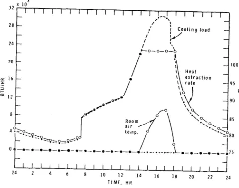
Fig. 4 shows the temperature at s o m e of the surfaces in the room. These w e r e calculated in the s a m e way a s the cooling load, except that s u r - face temperature response factors w e r e used in- stead of cooling load response factors. The curves show the extent to which the temperature of room s u r f a c e s can deviate f r o m the controlled room a i r temperature. It is obvious that occupants of this room would be uncomfortable during the afternoon in spite of the constant 75 F a i r temperature. CALCULATION O F ROOhl AIR T E M P E R A T U R E The response factor method can a l s o be used to compute room a i r temperature if the capacity of
1 1 1 1 1 ] 1 1 1 1 1 1 1 , , , , 1 Fig. 5 Room air temperature when I l l 1
maximum heat extraction i s l e s s
2 4 6 8 10 1 2 1 4 16 1 8 20 2 2 24
T I M E , H R than peak cooling load
the cooling s y s t e m i s l e s s than the p e a k cooling load o r if the cooling s y s t e m i s shut off during s o m e hours of the day. The data f o r t h i s calcula- tion a r e : the total cooling load, CL; the heat ex- traction, Q; and the cooling load r e s p o n s e f a c t o r s f o r a variation of r o o m a i r t e m p e r a t u r e , desig- nated P. The difference between the r o o m a i r t e m p e r a t u r e and t h e constant value assumed f o r the cooling load calculation i s 8. Each of these quantities i s a t i m e - s e r i e s and the corresponding lower c a s e l e t t e r with subscript indicates a t e r m in the s e r i e s .
Let
The deviation $equals en* when the l a t t e r i s posi- tive, and 8 = 0 f o r all t i m e s when en* is negative
n
if the cooling s y s t e m is under thermostatic con- t r o l . In the latter c a s e i t is assumed that the con- t r o l s y s t e m will adjust qn to make the quantity in-
..
s i d e the bracket z e r o if i t can.Fig. 5 shows how the a i r t e m p e r a t u r e would v a r y in the r o o m considered in the previous ex- ample if the maximum extraction r a t e of t h e cool- ing s y s t e m w e r e only 75% of the peak cooling load. This type of calculation can be modified quite e a s -
ily to allow f o r q a s a function of 8 if t h i s r e l a -
n n
tion i s known f o r the room cooling unit. ACCURACY.
No h a r d and fast statement c a n be made about t h e accuracy of the cooling load and s u r f a c e t e m p e r a - ture's calculated by the methods outlined above un- t i l they can be compared with values measured in an actual building. In the absence of t e s t r e s u l t s , however, s o m e indication of accuracy c a n be ob-
tained by comparing r e s u l t s obtained by the r e - sponse f a c t o r method with those obtained by other methods.
The cooling load f o r the room considered in t h e example w a s evaluated by two other methods: a n analog computer simulation and finite differ- ence calculations using a t i m e increment of 1/2 h r
.
The response factor and analog r e s u l t s agreed to within about I%, which i s comparable with t h e accuracy of the analog components. The finite dif-
f e r e n c e method gave a maximum cooling load about 10% l e s s than that indicated by the othei- methods. The following assumptions a r e implicit in all of these methods s o that comparison in no way val- idates them:1. Air temperature i s uniform throughout the room.
2. The floor, ceiling, walls and windows a r e isothermal surfaces; no account i s taken of devia- tions f r o m one -dimensional heat flow near the in- t e r s e c t i o n s between various enclosing s u r f a c e s .
3 . Convective heat t r a n s f e r coefficients a r e constant over each isothermal surface.
4. Furniture has no heat s t o r a g e capacity. The only significant variation among the t h r e e methods is i n the way they allow for transient heat conduction. The close agreement between the r e - s u l t s obtained by the response factor method and the analog computer lends confidence that both methods a r e reasonably good i n allowing for t r a n - sient heat conduction. I t is reasonable a l s o to as- s u m e that the finite difference approximations for the p a r t i a l derivatives lead to s o m e e r r o r , and these r e s u l t s suggest that the finite difference r e - s u l t s e r r on the non-conservative side. In any c a s e , computation required by the finite difference method i s s o much g r e a t e r than that required by the response factor method that t h e r e is no reason t o use finite differences except when the s y s t e m is non-linear
.
CONCLUSION
The t i m e - s e r i e s and response f a c t o r techniques make it practical t o use digital computers in a i r - conditioning calculations. The r e s u l t s a r e a s a c -
c u r a t e a s those obtained by analog computer; but experimental work i s needed t o confirm the apt- n e s s of the assumptions involved in a l l methods of computing cooling loads and s u r f a c e t e m p e r a t u r e s . This p a p e r i s a contribution f r o m the Division of Building Research, National R e s e a r c h Council, Canada, and i s published with the approval of t h e D i r e c t o r of the Division.
REFERENCES
1. Mitalas, G . P . , An Assessment of Common Assump- tions in Estimating Cooling Loads and Space Tem- peratures. ASHRAE Transactions; Vol. 7 1, P a r t 11, p. 72, 1965.
2. Tustin, A., A Method of Analyzing the Behaviorof Linear Systems in T e r m s of Time Series. J. , Inst. Elec. Engineers, Vol. 94, P a r t I1
-
A , No. 1, p. 130-142, 1947.3. Nessi, A. and L. Nisolle, Regimes Variables de Fonctionnement dans l e s Installations de Chauffage Central, 1925.
4. Hill, P. R , A. Method of Computing the Transient Temperature of Thick Walls f r o m Arbitrary Vari- ation of Adiabatic-Wall. Temperature and Heat- T r a n s f e r Coefficient. Nat. Atlvisory Committee for Aeronautics. Tech. Note 4105. 1957.
5. Brisken, W. R. and S. G. Reque, Heat Load Calcula- tions by Thermal Response. ASHRAE Transactions, Vol. 62, p. 391-4%, 1956.
6. Mitalas, G . P . and 13. G. Stephenson, Room Thermal Response Factors. ASHRAE Transactions, Vol. 73, P a r t I, 1967.
DISCUSSION
CHAIRMAN STOECKER: We will hold discussion mit the authors to answer the questions and com- on this paper until a f t e r we have had a chance to m e n t s together. (The companion paper follows. h e a r the companion paper, and then we will p e r - Ed. )
REPRINTED FROM THE ASHRAE TRANSACTIONS, 1967 VOLUME 73, PART 1, BY PERMISSION OF THE AMERICAN SOCIETY OF HEATING, REFRIGERATING, AND AIR-CONDITIONING ENGI- NEERS, INC. ASHRAE DOES NOT NECESSARILY AGREE WITH OPINIONS EXPRESSED AT ITS MEETINGS OR PRINTED IN ITS PUBLICATIONS.