HAL Id: hal-01403036
https://hal.inria.fr/hal-01403036
Submitted on 25 Nov 2016
HAL is a multi-disciplinary open access
archive for the deposit and dissemination of
sci-entific research documents, whether they are
pub-lished or not. The documents may come from
teaching and research institutions in France or
abroad, or from public or private research centers.
L’archive ouverte pluridisciplinaire HAL, est
destinée au dépôt et à la diffusion de documents
scientifiques de niveau recherche, publiés ou non,
émanant des établissements d’enseignement et de
recherche français ou étrangers, des laboratoires
publics ou privés.
equations with white noise dispersion
David Cohen, Guillaume Dujardin
To cite this version:
David Cohen, Guillaume Dujardin. Exponential integrators for nonlinear Schrödinger equations with
white noise dispersion. Stochastics and Partial Differential Equations: Analysis and Computations,
Springer US, 2017, pp.592-613. �10.1007/s40072-017-0098-1�. �hal-01403036�
EQUATIONS WITH WHITE NOISE DISPERSION
DAVID COHEN∗ANDGUILLAUME DUJARDIN†
Abstract.This article deals with the numerical integration in time of the nonlinear Schrödinger equation with power law nonlinearity and random dispersion. We introduce a new explicit exponential integrator for this purpose that integrates the noisy part of the equation exactly. We prove that this scheme is of mean-square order 1 and we draw consequences of this fact. We compare our exponential integrator with several other numerical methods from the literature. We finally propose a second exponential integrator, which is implicit and symmetric and, in contrast to the first one, preserves the L2-norm of the solution.
Key words.Stochastic partial differential equations; Nonlinear Schrödinger equation; White noise dispersion; Numerical methods; Geometric Numerical Integration; Exponential integrators; Mean-square convergence
AMS subject classifications.65C30; 65C50; 65J08; 60H15; 60-08
1. Introduction. We consider the time discretisation of the following nonlinear Schrödinger equation with white noise dispersion
idu + c∆u ◦ dβ+|u|2σu dt = 0
u(0) = u0, (1.1)
where the unknown u = u(x,t), with t≥ 0 and x ∈ Rd, is a complex valued random process, ∆u =
∑
dj=1
∂2u
∂x2
j
denotes the Laplacian inRd, c is a real number,σis a positive integer, andβ=
β(t) is a real valued standard Brownian motion. This stochastic partial differential equation is understood in the Stratonovich sense, using the◦ symbol for the Stratonovich product.
The existence of a unique global square integrable solution to (1.1) was shown in [13] forσ < 2/d and in [14] for d = 1 andσ= 2, see also [3]. The existence and uniqueness of solutions to the one-dimensional cubic case of the above problem was also studied in [25]. Furthermore, as for the deterministic Schrödinger equation, the L2-norm, or mass, of the solution to (1.1) is a conserved quantity. This is not the case for the total energy of the problem.
We now review the literature on the numerical analysis of the nonlinear Schrödinger equation with white noise dispersion (1.1). The early work [17] studies the stability with re-spect to random dispersive fluctuations of the cubic Schrödinger equation. Furthermore, nu-merical experiments using a split step Fourier method are presented. The paper [25] presents a Lie-Trotter splitting integrator for the above problem (1.1). The mean-square order of conver-gence of this explicit numerical method is proven to be at least 1/2 for a truncated Lipschitz nonlinearity [25, Sect. 5 and 6]. Furthermore, [25] conjectures that this splitting scheme should have order one, and supports this conjecture numerically. An analysis of asymptotic preserving properties of the Lie-Trotter splitting is carried out in [15] for a more general nonlinear dispersive equation. Very recently, the authors of [3] studied an implicit Crank-Nicolson scheme for the time integration of (1.1). They show that this scheme preserves the L2-norm and has mean-square order one of convergence in probability.
∗Department of Mathematics and Mathematical Statistics, Umeå University, SE–901 87 Umeå, Sweden
([email protected]). Department of Mathematics, University of Innsbruck, A–6020 Innsbruck, Austria ([email protected])
†Inria Lille Nord-Europe and Laboratoire Paul Painlevé UMR CNRS 8524, 59650 Villeneuve d’Asq Cedex,
In the present publication, we will consider exponential integrators for an efficient time discretisation of the nonlinear stochastic Schrödinger equation (1.1). Exponential integrators for the time integration of deterministic semi-linear problems of the form ˙y = Ly + N(y), are nowadays widely used and studied, as witnessed by the recent review [21]. Applications of such numerical schemes to the deterministic (nonlinear) Schrödinger equation can be found in, for example, [20, 5, 4, 9, 16, 10, 7, 8, 6] and references therein. Furthermore, these numerical methods were investigated for stochastic parabolic partial differential equations in, for example, [23, 22, 24], more recently for the stochastic wave equations in [11, 26, 12, 2], where they are termed stochastic trigonometric methods, and lately to stochastic Schrödinger equations driven by Ito noise in [1].
The main result of this paper is a mean-square convergence result for an explicit and easy to implement exponential integrator for the time discretisation of (1.1). Indeed, we will show in Section 3 convergence of mean-square order one for this scheme as well as convergence in probability. Note that the proofs of the results presented here use similar techniques as the one used in [3].
In order to show the above convergence result, we begin the exposition by introducing some notations and recalling useful results in Section 2. After that, we present our explicit exponential integrator for the numerical approximation of the above stochastic Schrödinger equation and analyse its convergence in Section 3. Various numerical experiments illustrating the main properties of our numerical scheme will be presented in Section 4. In the last section, we discuss the preservation of the mass, or L2-norm, by symmetric exponential integrators.
2. Notation and useful results. We denote the classical Lebesgue space of complex functions by L2:= L2(Rd,C), endowed with its real vector space structure, and with the
scalar product
(u, v) := Re
∫
Rdu ¯v dx.
For s∈ N, we further denote by Hs:= Hs(Rd,C) the Sobolev space of functions in L2such that their s first derivatives are in L2. The Fourier transform of a tempered distribution v is denoted byF (v) or bv. With this, Hs is the Sobolev space of tempered distributions v such that (1 +|ζ|2)s/2bv∈ L2.
Next, we consider a filtered probability space (Ω,F ,P,{Ft}t≥0) generated by a
one-dimensional standard Brownian motionβ=β(t).
With the above definitions in hand, we can write the mild formulation of the stochastic nonlinear Schrödinger equation (1.1) (with the constant c = 1 for ease of presentation) [25, 13, 3]
u(t) = S(t, 0)u0+ i
∫ t
0
S(t, r)(|u(r)|2σu(r)) dr, (2.1)
with the random propagator S(t, r) expressed in the Fourier variables as F (S(t,r)v(r))(ζ) = exp(−i|ζ|2(β(t)−β(r)))bv(r)(ζ) for t≥ r ≥ 0,ζ∈ Rdand v a tempered distribution.
We finally collect some results that we will use in the error analysis presented in Sec-tion 3:
• The random propagator S(t,r) is an isometry in Hsfor any s, see for example [3].
• There is a constant C such that, for t ≥ 0, h ∈ (0,1) and r ∈ (t,t + h) and for any Ft
(2.46)])
E[∥S(r,t)v − v∥2
Hs]≤ ChE[∥v∥2Hs+2] (2.2)
∥E[(S(r,t) − I)v]∥2
Hs≤ Ch2E[∥v∥2Hs+4]. (2.3)
• Without much loss of generality, we will truncate the nonlinearity in (1.1) in Section 3. Therefore, we recall the following estimates. Let f be a function from Hsto Hs, which sends Hs+2 to itself and Hs+4 to itself, with f (0) = 0, twice continuously differentiable on those spaces, with bounded derivatives of order 1 and 2. Consider u a solution on [0, T ] of
u(r)− u(t) = S(r,t)u(t) − u(t) + i
∫ r t
S(r,σ) f (u(σ)) dσ.
Then, there exists a constant C, which depends on f , such that (see [3, Equations (2.30) and (2.44)]) E[∥u(r) − u(t)∥2 Hs]≤ Ch sup σ∈[0,T]E[∥u(σ )∥2 Hs+2] (2.4) E[∥u(r) − u(t)∥4 Hs]≤ Ch2 sup σ∈[0,T]E[∥u(σ )∥4Hs+2], (2.5)
with h, r,t as in the above point (provided that the right-hand side is finite).
3. Exponential integrator and mean-square error analysis. This section presents an explicit time integrator for (1.1), and further states and proves a mean-square convergence result for this numerical method. As a by-product result, we also obtain convergence in probability of the exponential integrator.
3.1. Presentation of the exponential integrator. Let T > 0 be a fixed time horizon and an integer N≥ 1. We define the step size of the numerical method by h = T/N and denote the discrete times by tn= nh, for n = 0, . . . , N. Looking at the mild solution (2.1) of the problem
(1.1) on the interval [tn,tn+1], and discretising the integral (by freezing the integrand at the
left-end point of this interval), one can iteratively define the following explicit exponential integrator
u0= u(0)
un+1= S(tn+1,tn)un+ ihS(tn+1,tn)(|un|2σun). (3.1)
We thus obtain a finite sequence of numerical approximations un≈ u(tn) of the exact solution
to the problem (1.1) at the discrete times tn= nh.
3.2. Truncated Schrödinger equation. As in [3], we introduce a cut-off function in order to cope with the nonlinear part of the stochastic partial differential equation (1.1): Let
θ∈ C∞(R
+) withθ≥ 0, supp(θ)⊂ [0,2] andθ≡ 1 on [0,1]. For k ∈ N∗and x≥ 0, we set θk(x) =θ(xk). Finally, one defines fk(u) =θk(∥u∥2Hs+4)|u|2σu.
Observe that, for s > d/2 andσ∈ N⋆, for a fixed k∈ N∗, fkis a bounded Lipschitz
func-tion from Hs to Hs which sends Hs+2 to Hs+2 and Hs+4 to Hs+4. It is twice differentiable on these spaces, with bounded and continuous derivatives of order 1 and 2. Thus one has a unique global adapted solution ukto the truncated problem in L∞(Ω,C ([0,T],Hs)) if the
ini-tial value u0∈ Hs, see [3]. Note that, with the assumptions above, uk∈ L∞(Ω,C ([0,T],Hs)) as soon as u0∈ Hs+2, and uk∈ L∞(Ω,C ([0,T],Hs+4)) as soon as u0∈ Hs+4.
The global solution uk∈ L∞(Ω,C ([0,T],Hs)) to the truncated problem solves uk(t) = S(t, 0)u0+ i
∫ t 0
and the exponential integrator takes the form uk0= u(0)
ukn+1= S(tn+1,tn)ukn+ ihS(tn+1,tn) fk(ukn). (3.3)
Note that this method looks like the composition of two methods : The first is the explicit Euler equation applied to the differential equation u′= fk(u), the second is the exact solution
of the linear stochastic Schrödinger equation.
3.3. Main result and convergence analysis. This subsection states and proves the main result of this paper on the mean-square convergence of the exponential integrator applied to the nonlinear Schrödinger equation with white noise dispersion (1.1).
THEOREM 3.1. Let us fix s > d/2, the initial value u0∈ Hs+4(Rd) and an integer k≥ 1. Consider the unique adapted truncated solution of the random nonlinear Schrödinger equation uk(t) given by (3.2) with path a.s. inC ([0,T],Hs+4(Rd)). Further, consider the numerical solutions{ukn}, n = 0,1,...,N, given by the explicit exponential integrator (3.3) with step size h. One then has the following error estimate
∀h ∈ (0,1), sup
n|nh≤TE[∥u
k
n− uk(tn)∥2Hs]≤ Ch2
for the discrete times tn= nh. Here, the constant C does not depend on n, h with nh≤ T but may depend on k, T, supt∈[0,T]E[∥uk(t)∥4s+2], supt∈[0,T]E[∥uk(t)∥2s+4].
Proof. For ease of presentation, we will ignore the index k refereeing to the cut-off in the notations of the numerical and exact solutions as well as in the nonlinear function fk. But
we keep in mind that the constants below may depend on this index. We denote by C such a constant, providing it does not depend on n∈ N nor on h ∈ (0,1) such that nh ≤ T.
In order to later apply a discrete Gronwall-type argument, we first look at the error be-tween the exact and numerical solutions
en+1:= u(tn+1)− un+1= S(tn+1,tn)en+ ihS(tn+1,tn) ( f (u(tn))− f (un) ) − i∫ tn+1 tn ( S(tn+1,tn) f (u(tn))− S(tn+1, r) f (u(r) ) dr = S(tn+1,tn)en+ ihS(tn+1,tn) ( f (u(tn))− f (un) ) − i∫ tn+1 tn ( S(tn+1,tn)− S(tn+1, r) ) f (u(tn)) dr− i ∫ tn+1 tn S(tn+1, r) ( f (u(tn)− f (u(r) ) dr =: I1+ I2+ I3+ I4.
The so-called mean-square error thus reads E[∥en+1∥2s] = 4
∑
j=1 E[∥Ij∥2s] + 2 4∑
j=1 4∑
k= j+1 E[Re(Ij, Ik)s], (3.4)with the Hsnorm∥·∥2s = Re(·,·)s=∥·∥2Hs.
We now proceed with the estimations of the above quantities. Before estimating the mixed terms in (3.4), we start with the first four terms. By isometry of the random propagator S(t, r), one gets
For the second term, we again use the isometry property of the free random propagator and further the fact that the function f is Lipschitz. This gives us
E[∥I2∥2s] =E[∥hS(tn+1,tn)
(
f (u(tn))− f (un)
) ∥2
s] = h2E[∥ f (u(tn))− f (un)∥2s]≤ Ch2E[∥en∥2s].
Using the isometry property of S(t, r), Cauchy-Schwarz’s inequality, the estimate (2.2) from Section 2, and the fact that the exact solution is bounded, we can bound the third term by
E[∥I3∥2s] =E[∥ ∫ t n+1 tn S(tn+1,tn)(I− S(tn, r)) f (u(tn)) dr∥2s] ≤ E[( ∫ tn+1 tn 1· ∥S(tn+1,tn)(I− S(tn, r)) f (u(tn))∥sdr )2 ] ≤ h∫ tn+1 tn E[∥(I − S(tn, r)) f (u(tn))∥2s] dr = h ∫ tn+1 tn E[∥S(tn, r)(S(r,tn)− I) f (u(tn))∥2s] dr ≤ Ch2 ∫ tn+1 tn
E[∥ f (u(tn))∥2s+2] dr≤ Ch3 sup
t∈[0,T]E[∥u(t)∥
2
s+2]≤ Ch3.
In order to estimate the fourth term, we use the isometry property of the free random prop-agator, Cauchy-Schwarz’s inequality, the fact that f is Lipschitz, the estimate (2.4) on the time-variations of the exact solution, and the fact that the exact solution is bounded which is recalled in Section 2. We then obtain
E[∥I4∥2s] =E[∥ ∫ t n+1 tn S(tn+1, r) ( f (u(tn))− f (u(r)) ) dr∥2s] ≤ Ch ∫ tn+1 tn
E[∥ f (u(tn))− f (u(r))∥2s] dr≤ Ch
∫ tn+1 tn E[∥u(tn)− u(r)∥2s] dr ≤ Ch3 sup t∈[0,T]E[∥u(t)∥ 2 s+2]≤ Ch3.
Next, we go on with deriving bounds for the mixed terms present in (3.4). Using Cauchy-Schwarz’s inequality, the above bounds for the moments of I2and I3, and the fact that for all real numbers a, b, we have ab≤12(a2+ b2), we obtain the bound
|E[(I2, I3)s]| ≤ ( E[∥I2∥2s] )1/2(E[∥I 3∥2s] )1/2≤ Ch(E[∥e n∥2s] )1/2 h3/2≤ C(hE[∥en∥2s] + h4).
Similarly, one has
|E[(I2, I4)s]| ≤ C(hE[∥en∥2s] + h4)
and
|E[(I3, I4)s]| ≤ Ch3.
The term containing I1and I2can be estimated using Cauchy-Schwarz’s inequality and the fact that the function f is Lipschitz:
|E[(I1, I2)s]| = E[(S(tn+1,tn)en, ihS(tn+1,tn)
( f (u(tn))− f (un) ) )s] ≤(E[∥en∥2s] )1/2 h(E[∥ f (u(tn))− f (un)∥2s] )1/2 ≤ ChE[∥en∥2s].
The last two terms|E[(I1, I3)s]| and |E[(I1, I4)s]| demand more work. For the first one, we use
the isometry of the random propagator S(t, r) and Cauchy-Schwarz’s inequality to get: E[(I1, I3)s] = E[(S(tn+1,tn)en,
∫ tn+1 tn S(tn+1,tn)(I− S(tn, r)) f (u(tn)) dr)s = E[(en, ∫ tn+1 tn (I− S(tn, r)) f (u(tn)) dr)s ≤ h1/2( ∫ t n+1 tn |E[(en, (I− S(tn, r)) f (u(tn)))s]|2dr )1/2 .
We next apply the law of total expectation and again Cauchy-Schwarz’s inequality in order to get
E[(I1, I3)s] ≤h1/2
(∫ tn+1
tn
|E[(en,E{(I − S(tn, r)) f (u(tn))|Ftn})s]|
2dr)1/2
≤ h1/2(∫ tn+1 tn
E[∥en∥2s]· E[∥E{(I − S(tn, r)) f (u(tn))|Ftn}∥
2 s] dr
)1/2 . Finally, using (2.3) and the fact that the exact solution is bounded, one obtains the bound
E[(I1, I3)s] ≤Ch1/2 ( E[∥en∥2s] )1/2 h (∫ t n+1 tn E[∥ f (u(tn))∥2s+4] dr )1/2 ≤ Ch2(E[∥e n∥2s] )1/2( sup t∈[0,T]E[∥ f (u(t))∥ 2 s+4] )1/2 ≤ Ch2(E[∥e n∥2s] )1/2 ≤ C(h3+ hE[∥e n∥2s]).
In order to estimate the last term|E[(I1, I4)s]|, we use the mild formulation u(r)− u(tn) = S(tn, r)u(tn)− u(tn) + i
∫ r tn S(tn,θ) f (u(θ)) dθ = (S(tn, r)− I)u(tn) + i ∫ r tn S(tn,θ) f (u(θ)) dθ,
and then Cauchy-Schwarz’s inequality and a Taylor expansions of f∈ Cb2(Hs, Hs) to arrive
at |E[(I1, I4)s]| = E[(S(tn+1,tn)en, ∫ tn+1 tn S(tn+1, r)( f (u(tn))− f (u(r)))dr)s] = ∫ tn+1 tn
1· E[(en, S(tn, r)( f (u(tn))− f (u(r))))s] dr
≤ Ch1/2(
∫ tn+1
tn
|E[(en, S(tn, r)( f (u(tn))− f (u(r))))s]|2dr
)1/2 ≤ Ch1/2( ∫ tn+1 tn E[(en, S(tn, r) {
D f (u(tn))(u(r)− u(tn))
} )s] 2 dr )1/2 +Ch1/2 (∫ tn+1 tn |E[(en, S(tn, r) {∫ 1 0 D2f (θu(r) + (1−θ)u(tn)) dθ × (u(r) − u(tn), u(r)− u(tn))
} )s]|2dr )1/2 ≤ Ch1/2(∫ tn+1 tn |E[J1]|2dr )1/2 +Ch1/2 (∫ tn+1 tn |E[J2]|2dr )1/2 .
It thus remains to bound the above two terms. In order to start to estimate the first term, we insert the mild solution and obtain
h1/2 (∫ tn+1 tn |E[J1]|2dr )1/2 ≤ h1/2( ∫ tn+1 tn |E[(en, S(tn, r)D f (u(tn)) { (S(tn, r)− I)u(tn) + i ∫ r tn S(tn,θ) f (u(θ)) dθ } )s]|2dr )1/2 ≤ h1/2(∫ tn+1 tn
E[(en, S(tn, r)D f (u(tn))
{ (S(tn, r)− I)u(tn) } )s] 2 dr )1/2 + h1/2 (∫ tn+1 tn E[(en, S(tn, r)D f (u(tn)) {∫ r tn S(tn,θ) f (u(θ)) dθ } )s] 2dr )1/2 . We can now apply Cauchy-Schwarz’s inequality, the fact that S, f , D f are bounded and the
regularity estimate (2.3) from Section 2 to arrive at h1/2 (∫ tn+1 tn |E[J1]|2dr )1/2 ≤ Ch1/2(∫ tn+1 tn
E[∥en∥2s]E[∥(S(tn, r)− I)u(tn)∥2s] dr
)1/2 +Ch1/2 (∫ tn+1 tn E[∥en∥2s]E[∥ ∫ r tn S(tn,θ) f (u(θ)) dθ∥2s] dr )1/2 ≤ Ch1/2(E[∥e n∥2s])1/2h1/2h sup t∈[0,T] (E[∥u(t)∥2s+4])1/2 +Ch1/2(E[∥en∥2s])1/2 (∫ tn+1 tn (r−tn)2dr )1/2 ≤ Ch2(E[∥e n∥2s])1/2 ( 1 + sup t∈[0,T](E[∥u(t)∥ 2 s+4])1/2 ) ≤ C(h3+ hE[∥e n∥2s]) ( 1 + sup t∈[0,T] (E[∥u(t)∥2s+4])1/2).
For the second term, we again use Cauchy-Schwarz’s inequality with the fact that S, D f and D2f are bounded and the bound (2.5):
h1/2 (∫ tn+1 tn |E[J2]|2dr )1/2 ≤ Ch1/2( ∫ tn+1 tn
E[∥en∥2s]E[∥u(r) − u(tn)∥4s] dr
)1/2 ≤ Ch1/2(E[∥e n∥2s])1/2h1/2h sup t∈[0,T] (E[∥u(t)∥4s+2])1/2 ≤ Ch2(E[∥e n∥2s])1/2 sup t∈[0,T](E[∥u(t)∥ 4 s+2])1/2 ≤ C(h3+ hE[∥e n∥2s]) sup t∈[0,T] (E[∥u(t)∥4s+2])1/2. Altogether, we arrive at
E[(I1, I4)s] ≤C(h3+ hE[∥en∥2s])
( 1 + sup t∈[0,T] (E[∥u(t)∥4s+2])1/2+ sup t∈[0,T] (E[∥u(t)∥2s+4])1/2 ) . Collecting all the above bounds, the mean-square error (3.4) can thus be estimated by
E[∥en+1∥2s]≤ (1 + K1h + K2h2)E[∥en∥2s] + K3h3+ K4h4 and an application of a discrete Gronwall lemma gives the final bound
which concludes the proof of the theorem.
Using the above mean-square convergence result and similar arguments as in [25, 18] or [3], one can also show that the exponential method (3.1) has order of convergence one in probability.
PROPOSITION 3.2. Let T > 0 and assume that u0∈ Hs+4(Rd) with s > d/2 is such that the nonlinear Schrödinger equation with white noise dispersion (1.1) possesses a unique adapted solution u with paths a.s. inC ([0,T],Hs+4(Rd)). Let us apply the stochastic expo-nential integrator (3.1) to compute unwith step size h = T /N. Then, one has
lim C→+∞P ( max n=0,...,N∥u(tn)− un∥s≥ Ch ) = 0 uniformly in h, where we recall that tn= nh.
4. Numerical experiments. This section presents various numerical experiments for the nonlinear Schrödinger equation with white noise dispersion (1.1). We will use the follow-ing numerical schemes:
1. The explicit exponential integrator (3.1); 2. The Lie-Trotter splitting
u∗= S(tn+1,tn)un
un+1= Y (h)u∗ (4.1)
from [25]. Here, Y (h)u∗denotes the value at time h of flow associated to the problem i∂u∂t+|u|2σu = 0 with initial datum u∗;
3. The Strang splitting
u∗= S(tn+ h/2,tn)un
bu= Y(h)u∗
un+1= S(tn+1,tn+ h/2)bu, (4.2)
where again Y (h) is defined as above; 4. The implicit Crank-Nicolson scheme
iun+1− un
h +
χn
√
h∆un+1/2+ g(un, un+1) = 0 (4.3)
from [3]. Here, we have set un+1/2=12(un+ un+1),χn=β(t
n+1√)−β(tn) h and g(u, v) = 1 σ+1 ( |u|2σ+2−|v|2σ+2 |u|2−|v|2 )( u+v 2 ) .
We will consider the stochastic partial differential equation (1.1) on the one and two di-mensional torus with periodic boundary conditions. The spatial discretisation is done by a pseudospectral method with M Fourier modes in 1d, and M2Fourier modes in 2d.
4.1. Numerical experiments in 1d. This subsection presents convergence plots for the above mentioned numerical methods applied to the nonlinear Schrödinger equation with white noise dispersion (1.1); space-time evolution plots; experiments illustrating the influence of the power nonlinearityσsupporting a conjecture proposed in [3]; and finally illustrations of the preservation of the L2-norm along numerical solutions.
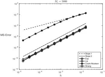
10-5 10-4 10-3 10-2 10-1 h 10-12 10-10 10-8 10-6 10-4 10-2 100 MS-Error Ms= 5000 Slope 1 Slope 2 Exp Lie Crank-Nicolson Strang
Figure 4.1: Mean-square errors for c = 1: Exponential integrator (□), Lie-Trotter (♢), Crank-Nicolson (∗), Strang (◦). The dotted lines have slopes 1 and 2.
4.1.1. Convergence plots. In order to illustrate the mean-square convergence of the exponential integrator (3.3), we consider problem (1.1) on the interval [0, 2π] with parameters c =σ = 1. The initial datum is u0(x) = e−(x−π)
2
for x∈ [0,2π]. Furthermore, M = 28 Fourier modes are used for the spatial discretisation. The mean-square errorsE[∥u(x,Tend)− uN(x)∥2L2] at time Tend= 0.5 are displayed in Figure 4.1 for various values of the time step h = 2−ℓ for ℓ = 6, . . . , 17. Here, we simulate the exact solution u(x,t) with the exponential method, with a small time step hexact= 2−17. The expected values are approximated by computing averages over Ms= 5000 samples. We computed the estimate for the largest
standard errors to be 5.78· 10−4 for the Crank-Nicolson scheme and around 10−6 for the other numerical schemes. These estimates are far from optimal but we observed that using a larger number of samples (Ms= 10000) does not improve significantly the behaviour of
the convergence plots. This is also the case for the other convergence plots presented below. In Figure 4.1, we observe convergence of order 1 for the exponential integrator. This is in agreement with Theorem 3.1. The orders of convergence for the splitting schemes and for the Crank-Nicolson scheme are also seen to be 1.
Note that the explicit exponential method (3.3), as well as the Lie and Strang splitting methods (4.1)-(4.2) take full advantage of the exact integration of the stochastic linear part of the Schrödinger equation when one uses periodic boundary conditions and hence the spectral properties of the Laplace operator are exactly known. In contrast, the Crank-Nicolson scheme (4.3) does not integrate the stochastic part of the equation exactly. One can even argue that the error in the identity
1 + iX 1− iX = e
2iX+O(X3),
which is the cornerstone of the error analysis of the linear part of the Crank-Nicolson scheme applied to a Schrödinger equation, is fully under control in the deterministic case (when X =−h2ξ2, andξ is the Fourier variable), while it can be much higher in the stochastic case (when X =−c∆Wn
2 ξ2) even for small time steps. Once again, such an error corresponding directly to the stochastic part of the PDE is not present in the three other schemes (3.1), (4.1) and (4.2). This explains, in 1d as well as in higher dimension (see next section for numerical
10-5 10-4 10-3 10-2 10-1 h 10-12 10-10 10-8 10-6 10-4 10-2 100 MS-Error Ms= 5000 Slope 1 Slope 2 Exp Lie Crank-Nicolson Strang
Figure 4.2: Mean-square errors for c = 0.25: Exponential integrator (□), Lie-Trotter (♢), Crank-Nicolson (∗), Strang (◦). The dotted lines have slopes 1 and 2.
examples in dimension 2), the relatively poor behaviour of the Crank-Nicolson scheme in this situation (see Fig 4.1) even if c is of order 1. On the other, as observed in Figure 4.2, the good convergence behaviour of the Crank-Nicolson is recovered for c = 0.25 (smaller noise intensity parameter). The other parameters are the same as in the previous numerical experiments.
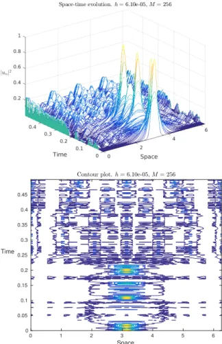
4.1.2. Evolution plots. Figure 4.3 shows the evolution of|un|2along one sample of the
numerical solution obtained by the exponential integrator (3.1) for the above problem with the discretisation parameters h = 2−14and M = 28. This illustrates, in the caseσ = 1, the interplay and the balance between the random dispersion and the nonlinearity. In contrast, the qualitative behaviour is different for higher values ofσ.
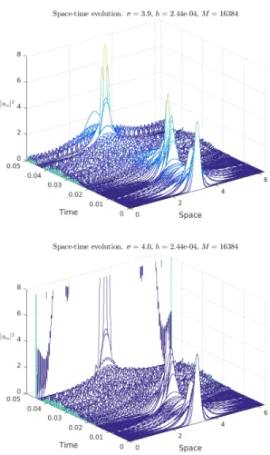
The article [3] conjectures that the power nonlinearityσ= 4 is the critical case for (1.1) in dimension one. We now present numerical experiments supporting this conjecture. Prob-lem (1.1) with the initial value u0(x) = 2.3· e−14(x−π)
2
is integrated over the time interval [0, 0.05] with discretisation parameters h = 2−12and M = 214. Figure 4.4 shows the space-time evolution for the power nonlinearityσ= 3.9 andσ= 4. Blow-up of the solution can be observed in the critical caseσ= 4 thus numerically confirming the conjecture from [3]. Of course, this is only a rough result and one can think of more sophisticated techniques such as adaptive mesh refinement techniques to have a better understanding of the behaviour of the solution close to the blow-up.
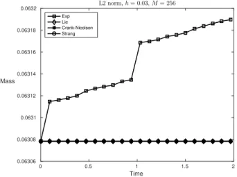
4.1.3. Preservation of the L2-norm. It is known that the L2-norm of the solution to the SPDE (1.1) remains constant for all times [3]. Figure 4.5 illustrates the corresponding preservation properties of the above numerical integrators along one sample path. For this numerical experiment, we consider the parameters c = 1,σ = 1, h = 2−5, M = 28 and the initial value u0(x) = e−10(x−π)
2
for x∈ [0,2π]. Exact preservation of the L2-norm for the splitting schemes and for the Crank-Nicolson scheme is observed, whereas a small drift is observed for the exponential integrator (3.1). In Section 5, we will propose a symmetric exponential integrator that preserves exactly the L2-norm.
Contour plot. h = 6.10e-05, M = 256 0 1 2 3 4 5 6 Space 0 0.05 0.1 0.15 0.2 0.25 0.3 0.35 0.4 0.45 Time
Figure 4.3: Space-time evolution (up) and contour plot (bottom) for the exponential integrator (3.3).
4.2. Numerical experiments in 2d. This subsection presents convergence plots for (1.1) in two dimensions as well as experiments illustrating the influence of the power nonlin-earityσsupporting a conjecture proposed in [3].
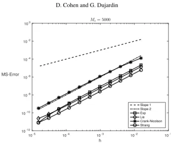
4.2.1. Convergence plots. We illustrate the mean-square convergence of the exponen-tial integrator (3.1) in 2d. To do so, we consider the problem (1.1) on [0, 2π]× [0,2π] with parameters σ = 1 and c = 1 or c = 0.1. The initial value is set to be u0(x, y) = e−((x−π/2)2+(y−π/2)2)ei10x+ e−0.5((x−3π/2)2+(y−3π/2)2)e−i10yfor (x, y)∈ [0,2π]× [0,2π]. Fur-thermore, M = 26 Fourier modes are used in each directions for the spatial discretisation. The temporal errors at time Tend= 0.5 are displayed in Figure 4.6 for various values of the time step h = 2−ℓ for ℓ = 15, . . . , 23. Here, we simulate the exact solution u(x, y,t) with a small time step hexact= 2−23. The expected values are approximated by computing averages over Ms= 25 samples (for these computationally expensive simulations). In this figure, we
observe convergence of order 1 for the exponential integrator. This is in agreement with Theorem 3.1.
Figure 4.4: Space-time evolution for the exponential integrator: σ = 3.9 (up) andσ = 4 (bottom).
4.2.2. Evolution plots. Let us now consider the following parameters c = 1, h = 2−11, M = 27and the initial value 5·e−14((x−π/2)2+(y−π/2)2)
·ei10xfor (x, y)∈ [0,2π]×[0,2π]. Figure 4.7 displays snapshots of the numerical solutions for the Schrödinger equation with power non-linearityσ = 1.9 andσ = 2. Blow-up of the solution can be observed numerically in the conjectured critical caseσ= 4/d = 2 from [3].
5. L2-preserving exponential integrators. As seen above, the proposed explicit expo-nential integrator unfortunately does not preserve the L2-norm. This can be fixed by consid-ering symmetric exponential integrators using ideas from [9]. We thus propose the follow-ing symmetric exponential method for the numerical discretisation of nonlinear Schrödfollow-inger
0 0.5 1 1.5 2 Time 0.06306 0.06308 0.0631 0.06312 0.06314 0.06316 0.06318 0.0632 Mass L2 norm, h = 0.03, M = 256 Exp Lie Crank-Nicolson Strang
Figure 4.5: Preservation of the L2-norm: Exponential integrator (□), Lie-Trotter (♢), Crank-Nicolson (∗), Strang (◦). 10-7 10-6 10-5 10-4 h 10-14 10-12 10-10 10-8 10-6 10-4 10-2 100 MS-Error Ms= 25 Slope 1 Slope 2 Exp Lie Crank-Nicolson Strang 10-7 10-6 10-5 10-4 h 10-16 10-14 10-12 10-10 10-8 10-6 10-4 10-2 MS-Error Ms= 25 Slope 1 Slope 2 Exp Lie Crank-Nicolson Strang
Figure 4.6: Mean-square errors in 2d for c = 1 (left) and c = 0.1 (right): Exponential integra-tor (□), Lie-Trotter (♢), Crank-Nicolson (∗), Strang (◦). The dotted lines have slopes 1 and 2.
equation with white noise dispersion (1.1) u0= u(0) N∗= N(S(tn+ h 2,tn)un+ h 2N∗) un+1= S(tn+1,tn)un+ hS(tn+ h,tn+ h 2)N∗, (5.1)
where N(u) = i|u|2σu is the nonlinearity.
This numerical method preserves the L2-norm as seen in the following proposition.
PROPOSITION5.1. The exponential integrator (5.1) preserves the L2-norm, as does the
exact solution of the nonlinear Schrödinger equation with white noise dispersion (1.1). Proof. This proof is an adaptation of the proof stating conditions for a Runge-Kutta methods to preserve quadratic invariants, see [19, Section IV.2.1] and further [9].
0 6 5 10 6 |un|2 15 4 Y 20 4 X 25 2 2 0 0
(a) Snapshot at time 0
0 0.05 6 0.1 0.15 6 |un| 20.2 4 0.25 Y 4 0.3 X 2 2 0 0 (b) Snapshot at time 0.049 0 0.5 6 1 6 1.5 |un| 2 4 2 Y 4 2.5 X 2 2 0 0 (c) Snapshot at time 0.105 0 6 5 10 6 |un|2 15 4 Y 20 4 X 25 2 2 0 0 (d) Snapshot at time 0 0 6 0.1 0.2 6 |un|2 4 0.3 Y 4 X 0.4 2 2 0 0
(e) Snapshot at time 0.049
0 6 1 2 6 ×10¹⁶ |un|2 3 4 Y 4 4 X 2 2 0 0 (f) Snapshot at time 0.105
Figure 4.7: Snapshots of the evolution of the exponential integrator in 2d:σ = 1.9 (up) and
σ= 2 (bottom). Discretisation parameters: h = 2−11and M = 27. Note the scale on the z-axis on Figure 4.7f.
Let us compute the L2-norm of u1: ∥u1∥2=∥S(t1,t0)u0+ hS(t0+ h,t0+ h 2)N∗∥ 2=∥u 0∥2+ h2∥N∗∥2 + h ( S(t1,t0)u0, S(t0+ h,t0+ h 2)N∗ ) + h ( S(t0+ h,t0+ h 2)N∗, S(t1,t0)u0 ) using the isometry of the random propagator S(t, r). We next define Y := S(t0+h2,t0)u0+h2N∗ so that u0= S(t0,t0+h2)(Y−h2N∗). Inserting this quantity in the above equation and using the definition of S(t, r) yields
∥u1∥2=∥u0∥2+ h2∥N∗∥2− h2 2 ∥N∗∥ 2−h2 2 ∥N∗∥ 2+ h((Y, N ∗) + (N∗,Y ) ) =∥u0∥2
since the last term in brackets is zero (this follows from the fact that N∗= N(Y ) and the fact that the L2-norm is a first integral).
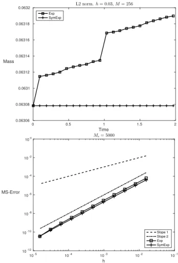
5.1. Numerical experiments for the symmetric exponential integrator. Figure 5.1 illustrates the preservation of the L2-norm by the exponential methods (3.1) and (5.1) as well as strong convergence plots. The parameter values are the same as in the above numerical experiments. Exact preservation of the L2-norm, as stated in Proposition 5.1, is observed for the symmetric version. The convergence plot indicates the same order of convergence for the symmetric version of the scheme as for the original exponential integrator (3.1).
6. Conclusion. We introduced a new, explicit, exponential integrator (3.1) for the time integration of the nonlinear Schrödinger equation with power-law nonlinearity and random
0 0.5 1 1.5 2 Time 0.06306 0.06308 0.0631 0.06312 0.06314 0.06316 0.06318 0.0632 Mass L2 norm. h = 0.03, M = 256 Exp SymExp 10-5 10-4 10-3 10-2 10-1 h 10-12 10-10 10-8 10-6 10-4 10-2 100 MS-Error Ms= 5000 Slope 1 Slope 2 Exp SymExp
Figure 5.1: Preservation of the L2-norm (top) and mean-square errors (bottom) for the sym-metric exponential integrator (5.1) (+) and for the exponential integrator (3.1) (□). The dotted lines have slopes 1 and 2.
dispersion (1.1). We showed that this integrator has mean-square order one (Theorem 3.1). We compared it with other methods from the literature. In contrast to methods such as the Lie-Trotter splitting or the Crank-Nicolson method, it does not preserve the L2-norm exactly (Figure 4.5). However, it shares the same order and our numerical experiments show that it outperforms methods that do not integrate exactly the linear part of the equation, such as the Crank-Nicolson method, in terms of size of constant errors, for reasonably large noise intensity (Figure 4.1). Furthermore, we used this new scheme in Section 4.2 to support a conjecture on the critical power to get blow-up in finite time in the nonlinear Schrödinger equation (1.1). Finally, we proposed another exponential integrator (5.1) which is symmetric and has the same numerical order as the one proposed initially. It however is implicit and hence has higher numerical cost.
[1] R. ANTON ANDD. COHEN, Exponential integrators for stochastic Schrödinger equations driven by ito noise, Submitted, (2016).
[2] R. ANTON, D. COHEN, S. LARSSON,ANDX. WANG, Full discretisation of semi-linear stochastic wave equations driven by multiplicative noise, To appear in SIAM J. Numer. Anal., (2016).
[3] R. BELAOUAR, A.DEBOUARD,ANDA. DEBUSSCHE, Numerical analysis of the nonlinear Schrödinger equation with white noise dispersion, Stoch. Partial Differ. Equ. Anal. Comput., 3 (2015), pp. 103–132. [4] H. BERLAND, A. L. ISLAS,ANDC. M. SCHOBER, Conservation of phase space properties using exponential
integrators on the cubic Schrödinger equation, J. Comput. Phys., 225 (2007), pp. 284–299.
[5] H. BERLAND, B. OWREN,ANDB. SKAFLESTAD, Solving the nonlinear Schrödinger equation using expo-nential integrators, Modeling, Identification and Control, 27 (2006), pp. 201–218.
[6] C. BESSE, G. DUJARDIN, ANDI. LACROIX-VIOLET, High order exponential integrators for nonlinear Schrödinger equations with application to rotating Bose-Einstein condensates, preprint, (2015). [7] B. CANO ANDA. GONZÁLEZ-PACHÓN, Exponential time integration of solitary waves of cubic Schrödinger
equation, Appl. Numer. Math., 91 (2015), pp. 26–45.
[8] , Projected explicit Lawson methods for the integration of Schrödinger equation, Numer. Methods Partial Differential Equations, 31 (2015), pp. 78–104.
[9] E. CELLEDONI, D. COHEN,ANDB. OWREN, Symmetric exponential integrators with an application to the cubic Schrödinger equation, Found. Comput. Math., 8 (2008), pp. 303–317.
[10] D. COHEN ANDL. GAUCKLER, Exponential integrators for nonlinear Schrödinger equations over long times, BIT, 52 (2012), pp. 877–903.
[11] D. COHEN, S. LARSSON,ANDM. SIGG, A trigonometric method for the linear stochastic wave equation, SIAM J. Numer. Anal., 51 (2013), pp. 204–222.
[12] D. COHEN AND L. QUER-SARDANYONS, A fully discrete approximation of the
one-dimensional stochastic wave equation, IMA J NUMER ANAL, 36 (2016), pp. 400–420.
http://dx.doi.org/10.1093/imanum/drv006.
[13] A.DEBOUARD ANDA. DEBUSSCHE, The nonlinear Schrödinger equation with white noise dispersion, J. Funct. Anal., 259 (2010), pp. 1300–1321.
[14] A. DEBUSSCHE ANDY. TSUTSUMI, 1D quintic nonlinear Schrödinger equation with white noise dispersion, J. Math. Pures Appl. (9), 96 (2011), pp. 363–376.
[15] R. DUBOSCQ, Analyse et simulations numériques d’équations de Schrödinger déterministes et stochastiques. Applications aux condensats de Bose-Einstein en rotation, PhD thesis, Université de Lorraine, Nancy, 2013.
[16] G. DUJARDIN, Exponential Runge-Kutta methods for the Schrödinger equation, Appl. Numer. Math., 59 (2009), pp. 1839–1857.
[17] J. GARNIER, Stabilization of dispersion-managed solitons in random optical fibers by strong dispersion man-agement, Optics Communications, 206 (2002), pp. 411–438.
[18] M. GAZEAU, Probability and pathwise order of convergence of a semidiscrete scheme for the stochastic Manakov equation, SIAM J. Numer. Anal., 52 (2014), pp. 533–553.
[19] E. HAIRER, CH. LUBICH,ANDG. WANNER, Geometric numerical integration, vol. 31 of Springer Series in Computational Mathematics, Springer, Heidelberg, 2010. Structure-preserving algorithms for ordinary differential equations, Reprint of the second (2006) edition.
[20] M. HOCHBRUCK ANDC. LUBICH, Exponential integrators for quantum-classical molecular dynamics, BIT, 39 (1999), pp. 620–645.
[21] M. HOCHBRUCK ANDA. OSTERMANN, Exponential integrators, Acta Numer., 19 (2010), pp. 209–286. [22] A. JENTZEN ANDP. E. KLOEDEN, The numerical approximation of stochastic partial differential equations,
Milan J. Math., 77 (2009), pp. 205–244.
[23] G. J. LORD ANDJ. ROUGEMONT, A numerical scheme for stochastic PDEs with Gevrey regularity, IMA J. Numer. Anal., 24 (2004), pp. 587–604.
[24] G. J. LORD ANDA. TAMBUE, Stochastic exponential integrators for the finite element discretization of SPDEs for multiplicative and additive noise, IMA J. Numer. Anal., 33 (2013), pp. 515–543.
[25] R. MARTY, On a splitting scheme for the nonlinear Schrödinger equation in a random medium, Commun. Math. Sci., 4 (2006), pp. 679–705.
[26] X. WANG, An exponential integrator scheme for time discretization of nonlinear stochastic wave equation, Journal of Scientific Computing, (2014), pp. 1–30.