Interpretable time series kernel analytics by pre-image estimation

(1)

HAL Id: hal-03088295

https://hal-normandie-univ.archives-ouvertes.fr/hal-03088295

Submitted on 26 Dec 2020

HAL is a multi-disciplinary open access

archive for the deposit and dissemination of

sci-entific research documents, whether they are

pub-lished or not. The documents may come from

teaching and research institutions in France or

L’archive ouverte pluridisciplinaire HAL, est

destinée au dépôt et à la diffusion de documents

scientifiques de niveau recherche, publiés ou non,

émanant des établissements d’enseignement et de

recherche français ou étrangers, des laboratoires

Interpretable time series kernel analytics by pre-image

estimation

Thi Phuong Thao Tran, Ahlame Douzal-Chouakria, Saeed Varasteh Yazdi,

Paul Honeine, Patrick Gallinari

To cite this version:

Thi Phuong Thao Tran, Ahlame Douzal-Chouakria, Saeed Varasteh Yazdi, Paul Honeine, Patrick

Gallinari. Interpretable time series kernel analytics by pre-image estimation. Artificial Intelligence,

Elsevier, 2020, 286, pp.103342. �10.1016/j.artint.2020.103342�. �hal-03088295�

(2)

Interpretable time series kernel analytics by pre-image

1

estimation

2 Abstract 3

Kernel methods are known to be e↵ective to analyse complex objects by im-plicitly embedding them into some feature space. To interpret and analyse the obtained results, it is often required to restore in the input space the results ob-tained in the feature space, by using pre-image estimation methods. This work proposes a new closed-form pre-image estimation method for time series kernel analytics that consists of two steps. In the first step, a time warp function, driven by distance constraints in the feature space, is defined to embed time series in a metric space where analytics can be performed conveniently. In the second step, the time series pre-image estimation is cast as learning a linear (or a nonlinear) transformation that ensures a local isometry between the time se-ries embedding space and the feature space. The proposed method is compared to the state of the art through three major tasks that require pre-image estima-tion: 1) time series averaging, 2) time series reconstruction and denoising and 3) time series representation learning. The extensive experiments conducted on 33 publicly-available datasets show the benefits of the pre-image estimation for time series kernel analytics.

1. Introduction

4

Kernel methods [24] are well known to be e↵ective in dealing with

nonlin-5

ear machine learning problems in general, and are often required for machine

6

learning tasks on complex data as sequences, time series or graphs. The main

7

idea behind kernel machines is to map the data from the input space to a

8

higher dimension feature space (i.e., kernel space) via a nonlinear map, where

9

the mapped data can be then analysed by linear models. While the mapping

10

from input space to the feature space is of primary importance in kernel

meth-11

ods, the reverse mapping of the obtained results from the feature space back to

12

the input space (called the pre-image problem) is also very useful. Estimating

13

pre-images is important in several contexts for interpretation and analysis

pur-14

poses. From the beginning, it has been often considered to estimate denoised

15

and compressed results of a kernel Principal Component Analysis (PCA). Other

16

tasks are of great interest, since the pre-image estimation allows, for instance,

17

to obtain the reverse mapping of the centroids of a kernel clustering, and of the

18

atoms as well as of the sparse representations in kernel dictionary learning.

19 20

Thao Tran Thi Phuong, Ahlame Douzal, Saeed Varasteh Yazdi,

Paul Honeine, and Patrick Gallinari

(3)

In view of the importance of the pre-image estimation issue and of its

bene-21

fits in machine learning, several major propositions have been developed. First,

22

in Mika et al. [23], the problem is formalised as a nonlinear optimisation

prob-23

lem and, for the particular case of the Gaussian kernel, a fixed-point iterative

24

solution to estimate the reverse mapping is proposed. To avoid numerical

insta-25

bilities of the latter approach, in Kwok et al.[18], the relationship between the

26

distances in feature and input spaces is established for standard kernels, and

27

then used to approximate pre-images by multidimensional scaling. In Bakir et

28

al. [3], the pre-image estimation problem is cast as a regression problem

be-29

tween the input and the mapped data, the learned regression model is then

30

used to predict pre-images. Honeine and Richard proposed in [15] an approach

31

where the main idea is to estimate, from the mapped data, a coordinate system

32

that ensures an isometry with the input space; this approach has the advantage

33

to provide a closed-form solution, to be independent of the kernel nature and

34

to involve only linear algebra. More recently, task-specific estimation has been

35

studied, such as the resolution of the pre-image problem for nonnegative matrix

36

factorisation in [32].

37

All the proposed methods for pre-image estimation are either based on

op-38

timisation schema, such as gradient descent or fixed-point iterative solution, or

39

based on ideas borrowed from dimensionality reduction methods. In

particu-40

lar, these methods were developed for Euclidean input spaces, as derivations

41

are straightforward owing to linear algebra (see [16] for a survey on the

resolu-42

tion of the pre-image problems in machine learning). A major challenge arises

43

when dealing with non-Euclidean input spaces, that describe complex data as

44

sequences, time series, manifolds or graphs. Some recent works address that

45

pre-image problem on that challenging data. For instance, in Cloninger et al.

46

[9] the pre-image problem is addressed for Laplacian Eigenmaps under L1

reg-47

ularisation and in Bianchi et al. [6] an encoder-decoder is used to learn a latent

48

representation driven by the kernel similarities, where the pre-image estimation

49

is explicitly given by the decoder side.

50

For temporal data, while kernel machinery has been increasingly investigated

51

with success for time series analytics [13, 27, 31, 30, 29, 19], the pre-image

52

problem for temporal data remains in its infancy. In addition, time series data,

53

that involve varying delays and/or di↵erent lengths, are naturally lying in a

54

non-Euclidean input space, making the above existing pre-image approaches for

55

static data inapplicable. This work aims to fill this gap, by proposing a

pre-56

image estimation approach for time series kernel analytics, that consists of two

57

steps. In the first step, a time warp function, driven by distance constraints

58

in the feature space, is defined to embed time series in a metric space where

59

analytics can be performed conveniently. In the second step, the time series

60

pre-image estimation is cast as learning a linear or a nonlinear transformation

61

that ensures a local isometry between the time series embedding space and the

62

feature space. The relevance of the proposed method is studied through three

63

major tasks that require pre-image estimation: 1) time series averaging, 2) time

64

series reconstruction and denoising under kernel PCA, and 3) time series

repre-65

sentation learning and dictionary learning under kernel k-SVD. The benefits of

(4)

the proposed method are assessed through extensive experiments conducted on

67

33 publicly-available time series datasets, including univariate and multivariate

68

time series that may include varying delays and be of the di↵erent lengths.

69 70

The main contributions of this paper are:

71

1. We propose a time warp function, driven by distance constraints in the

72

feature space, that embeds time series into an Euclidean space

73

2. We cast the time series pre-image estimation approach as learning a linear

74

or nonlinear transformations in the feature space

75

3. We propose a closed-form solution for pre-image estimation by preserving

76

a local isometry between the temporal embedded space and the feature

77

space

78

4. We conduct wide experiments to compare the proposed approach to the

79

major alternative pre-image estimation methods under three crucial tasks:

80

1) time series averaging, 2) time series reconstruction and denoising and

81

3) time series representation and dictionary learning.

82

The reminder of the paper is organised as follows. Section 2 gives a brief

83

introduction to kernel PCA and kernel k-SVD and Section3presents the major

84

pre-image estimation methods. In Section 4, we formalise the pre-image

esti-85

mation problem for time series and develop the proposed solution as well as the

86

corresponding algorithm. We detail the experiments conducted and discuss the

87

obtained results in Section5.

88

2. Kernel PCA and kernel k-SVD

89

Kernel methods [24] rely on embedding samples xi 2 Rd with (xi) into a

90

feature spaceH, a Hilbert space of arbitrary large and possibly infinite

dimen-91

sion. The map function needs not to be explicitly defined, since computations

92

conducted inH can be carried out by a kernel function that measures the inner

93

product in that space, namely (xi, xi0) =h (xi), (xi0)i for all xi, xi0. Given

94

a set of input samples {xi}Ni=1, xi 2 Rd, let K be the Gram matrix related

95

to the kernel, namely Kii0 = (xi, xi0). Let X = [x1, ..., xN] 2 Rd⇥N be the

96

description of N input samples xi 2 Rd and, with some abuse of notation, let

97

(X) be the matrix of entries (x1), ..., (xN).

98 99

In the following, we describe two well-known kernel methods, kernel PCA

100

and kernel k-SVD, as nonlinear extensions of the well-known PCA and k-SVD.

101

While both methods estimate a linear combination for optimal reconstruction

102

of the input samples, the former forces the orthogonality of the atoms that leads

103

to an orthonormal basis, and the latter forces the sparsity while relaxing the

104

orthogonality condition.

105

2.1. Kernel PCA

106

Kernel PCA extends standard PCA to find principal components that are

107

nonlinearly related to the input variables. For that, the principal components

(5)

are rather determined in the feature space. For the sake of clarity, we assume

109

for now that we are dealing with centred mapped data, namelyPN_i=1 (xi) = 0.

110

The covariance matrix in the feature space takes then the form

111 C = 1 N N X i=1 (xi) (xi)T. (1)

Similarly to standard PCA, the objective comes to find the pairs of eigenvalue

112

j 0 and corresponding eigenvector uj2 H \ 0 that satisfy

113

juj= Cuj, (2)

namely for each (xi)

114

jhuj, (xi)i = hCuj, (xi)i. (3)

As each eigenvector uj lies in the span of (x1), ..., (xN), there exist

coeffi-115

cients ↵ij, ..., ↵N j such that

116 uj = N X i=1 ↵ij (xi). (4)

From Eq. (3) and Eq. (4), and by simple developments, the problem in Eq. (2)

117

remains to find the solution of the eigendecomposition problem:

118

j↵j = N1K↵j. (5)

Let 1 ... p be the p highest non-zero eigenvalues of _N1K and ↵1, ..., ↵p

119

their corresponding eigenvectors. The principal components in the feature space

120

are then given by computing the projections Pj( (x)) of the sample x onto the

121 eigenvector uj = (X) ↵j: 122 Pj( (x)) =huj, (x)i = N X i=1 ↵ijh (xi), (x)i = kx↵j (6)

with kx = [(x1, x), ..., (xN, x)]. By denoting ↵ = [↵1, ..., ↵p], the description

123

P ( (x)) of (x) into the subspace of the p first principal components is then

124

P ( (x)) = (kx↵)T (7)

Two considerations should be taken. First, the eigenvector expansion

coeffi-125

cients ↵j should be normalised by requiring jh↵j, ↵ji = 1. Secondly, as (xi)

126

are assumed centred, both the Gram matrix K in Eq. (5) and kx used in Eq.

127

(6) and Eq. (7) need to be substituted with their centred counterparts, namely

128 e Kij = (K 1NK K1N+ 1NK1N)ij (8) e kx = ⇣ kx _N1 1TNK ⌘ (IN 1N) (9)

with (1N)ij = 1/N for all i, j, IN the identity matrix and 1N 2 RN the unit

129

vector.

(6)

2.2. Kernel k-SVD

131

Sparse coding and dictionary learning become popular methods for a

vari-132

ety of tasks as feature extraction, reconstruction, denoising, compressed sensing

133

and classification [17,4,5]. k-SVD [1] is among the most-known and tractable

134

dictionary learning approach to learn a dictionary and to sparse represent the

135

input samples as a linear combination of the dictionary atoms. When

deal-136

ing with complex data, kernel k-SVD may be required to learn, in the feature

137

space, the dictionary and the sparse representations of the mapped samples as

138

a nonlinear combination of the dictionary atoms [28]. Let us introduce a brief

139

description of kernel k-SVD.

140 141

Let D = [d1, ..., dL]2 Rd⇥Lbe the dictionary composed of L atoms dj2 Rd.

142

The embedded dictionary (D) = (X)B is defined as a linear representation

143

of (X), since the atoms lie in the subspace spanned by the (X). The kernel

144

dictionary learning problem takes the form

145 min B,Ak (X) (X)B Ak 2 F (10) s.t.kaik0 ⌧ 8i = 1, ..., N, (11)

where k.kF is the Frobenius norm1, the matrix B = [ 1, ..., L] 2 RN⇥L

146

gives the representation of the embedded atoms into the base (X) and A =

147

[a1, ..., aN]2 RL⇥N gives the sparse representations of (X), with the sparsity

148

level ⌧ imposed by the above constraint.

149 150

The kernel k-SVD algorithm iteratively cycles between two stages. In the

151

first stage, the dictionary is assumed fixed withB known and a kernel

orthog-152

onal matching pursuit (OMP) technique [20] is deployed to estimateA. As in

153

standard OMP, given a sample x, we select the first atom that best reconstructs

154

(x); namely we select the j-th atom that maximises

155

kx aTxBTK j. (12)

The sparse codes are then updated by the projections onto the subspace of the

156

yet selected atoms

157

ax = B⌦TKB⌦

1

(kxB⌦)T, (13)

where BT

⌦ is the submatrix ofB limited to the yet selected atoms. The

proce-158

dure is reiterate until the selection of ⌧ atoms.

159 160

Once the sparse codesA of the N samples estimated, the second stage of the

161

kernel k-SVD is performed to update bothB and A. For that, the reconstruction

162

1_kMk

F=qPpi=1

Pq

j=1(mij)2is the Frobenius norm of the matrix M2 Rp⇥qof general

(7)

error is defined as 163 min B,Ak (X) (X) L X j=1 jaj.k2_F, (14)

with aj.2 RN referencing the j-th row ofA, namely

164

min

B,Ak (X)Ek (X) kak.k

2

F, (15)

with Ek= IN Pj6=k jaj. the error of reconstruction matrix when removing

165

the k-th atom. An eigendecomposition is then performed to get

166

(ERk)TK(ERk) = V ⌃VT, (16)

where ER

k is the error of reconstruction restricted to the samples that have

167

involved the k-th atom. The sparse codes k and aRk.are updated by using the

168

first eigenvector v1 with

169

aRk.= 1vT1 and k= 11EkRv1. (17)

3. Related works on pre-image estimation

170

From the representer theorem [22] any result '2 H obtained by some kernel

171

method may be expressed in the form ' = PN_i=1 i (xi); that is as a linear

172

combination of the mapped training samples { (xi)}Ni=1. In general, finding

173

the exact pre-image x such that (x) = ' is an ill-posed problem, that is often

174

addressed by providing an approximate solution, namely by estimating x⇤such

175

that (x⇤₎_{⇡ '. In the following, we describe three major methods to estimate}

176

the pre-image x⇤_{of a given '}_{2 H.}

177

3.1. Pre-image estimation under distance constraints

178

The main idea proposed in Kwok et al. [18] is to use the distances between

179

' and (xi) and their relation to the distances between the pre-image x⇤ and

180

xi. The main steps of the proposed approach are:

181

1. Let ed2_{(', (x}

i)) =h', 'i 2h', (xi)i+h (xi), (xi)i be the square

dis-182

tance between ' and any (xi). In practice, only neighbouring elements

183

are considered. Let ( ˙x1), ... ( ˙xn) denote the n-th closest elements to '.

184

2. For an isotropic kernel2_{, the relation d}2_(x

i, xj) = g( ed2( (xi), (xj)))

be-185

tween the distances in the input and the feature spaces can be established.

186

2_{an isotropic kernel is a function of the form k(x, y) = f (}_kx _y_{k) that depends only on}

(8)

3. A solution is then deployed to determine the pre-image x⇤ such that 187 [d2(x⇤, ˙x1), . . . , d2(x⇤, ˙xn)] = ⇥ g( ed2(', ( ˙x1))), ..., g( ed2(', ( ˙xn))) ⇤ . (18) For that, an SVD is deployed on the centred version of the submatrix

188

Xn= [ ˙x1, ..., ˙xn], namely

189

Xn(In 1n) = U ⇤VT, (19)

where U = [u1, . . . , uq] is the d⇥ q matrix of the left-singular vectors.

190

Let Z = [z1, . . . , zn] = ⇤VT be the q⇥ n matrix giving the projections of

191

˙

xi on the uj’s orthonormal vectors. The pre-image estimation x⇤is then

192

obtained as:

193

x⇤ = U z⇤+ 1

nXn1n, (20)

where z⇤_{, the projection of x}⇤_{on the [u}₁_{, ..., u}_q_{] coordinate system, is}

194 z⇤= 1 2(Z Z T₎ 1_{Z (d}2 _d2 0), (21) with d20= [kz1k2, ...,kznk2]T, d2= [d21, . . . , d2n]Tand d2i = g( ed2(', ( ˙xi))). 195

3.2. Pre-image estimation by isometry preserving

196

To learn the pre-image x⇤ _{of a given ' =} PN

i=1 i (xi), the proposed

197

approach in [15] proceeds in two steps. First, a coordinate system, spanned by

198

the feature vectors{ (xi)}Ni=1is learned to ensure an isometry with the input

199

space; subsequently, the coordinate system is used to estimate the pre-image x⇤

200

of '. These two main steps are summarised in the followings:

201

1. Let ={ 1, ..., p} (p  N) be a coordinate system in the feature space,

202

with k = (X)↵k. The projection of (X) onto the coordinate system

203

is P ( (X)) = (KA)T_{, where A = [↵}

1, ..., ↵p]. To estimate the coordinate

204

system that is isometric with the input space, the following optimisation

205 problem is solved 206 arg min A kX T_X _KAAT_K_k2 F + kKAk2F, (22)

where the second term controls through the regularisation parameter

207

the smoothness of the solution. The solution of this problem satisfies

208

AAT _{= K} 1_(XT_X _K 1_)K 1_.

209

2. Based on this result, the pre-image estimation x⇤_{takes the form}

210

x⇤= arg min

x kX

T_x _(XT_X _K 1₎ _k2

F (23)

with = ( 1, ..., N)T. This problem defines a standard overdetermined

211

equation system (N d) that can be resolved as a least-square

min-212

imisation problem (i.e., any technique such as the pseudo-inverse or the

213

eigendecomposition). The pre-image estimation is then:

214

(9)

3.3. Pre-image estimation by kernel regression

215

In Bakir et al. [3], the pre-image estimation consists in learning a kernel

216

regression function that maps all the (xi) in the feature spaceH (related to

217

the kernel ) to xiin the input spaceRd. For that, first a kernel PCA is deployed

218

to embed (X) into the subspace spanned by the eigenvectors u1, ..., updefined

219

in (4), with uj= (X)↵j. Then, a kernel regression is learned from the set of

220

the projections onto the kernel PCA subspace and X as

221

arg min

B kX B bKk 2

F+ kBk2F, (25)

where B2 Rd⇥N _{is the regression coefficient matrix and b}_{K is the Gram matrix}

222

with entries bKij=b(P ( (xi)), P ( (xj))). The solution to the problem (25) is

223

then

224

B = X bK( bK2+ IN) 1 (26)

For a given result ' = (X) 2 H, its pre-image x⇤_{is then estimated as:}

225 x⇤= BbkTP ('), (27) with 226 b kP (') = [b(P ('), P ( (x1))), ...,b(P ('), P ( (xN)))], (28) whereb(P ('), P ( (xi))) =b(↵TK , ↵TkTxi) and ↵ = [↵1, ..., ↵p]. 227 228 3.4. Overview 229

To sum up, the three major methods presented above define three di↵erent

230

approaches for pre-image estimation problem. First of all, all the methods

in-231

volve only linear algebra and propose solutions that don’t su↵er from numerical

232

instabilities. In Kwok et al. [18], the solution is mainly requiring the definition

233

of a relation between the distances into the input and the kernel feature spaces.

234

That requirement limite the Kwok et al. [18] approach to linear or isotropic

235

kernels. Honeine et al. [15] alleviate that point by proposing a closed-form

solu-236

tion that is applicable to any type of kernels. Furthermore, while in Honeine et

237

al. [15] the pre-image estimation is obtained by learning a linear transformation

238

into the feature space that preserves the isometry between the input and the

239

feature space, in Bakir et al. [3], the pre-image estimation is obtained by using

240

a non linear kernel regression that predicts the input samples from their images

241

into the feature space. Finally, while both [15] and [3] proposals involve the

242

whole training samples for pre-image estimation, Kwok et al. [18] uses only the

243

samples on the neighborhood of ', which o↵ers a significant speed-up; highly

244

valuable in the case of large scale data.

(10)

4. Proposed pre-image estimation for time series kernel analytics

246

Let {xi}Ni=1 be a set of N time series, where each xi 2 Rd⇥ti is a

mul-247

tivariate time series of length ti that may involve varying delays. Let (xi)

248

be the -mapping of the time series xi into the Hilbert space H related to a

249

temporal kernel  that involves dynamic time alignments such as dtak [25],

250

kdtw [2] and kga [10]. Let K be a the corresponding Gram matrix, with

251

entries Kii0 = (xi, xi0). Given ' = PN_i=1 i (xi) a result generated in H,

252

the objective is to estimate the time series x⇤ 2 Rd⇥t⇤

that is the pre-image

253

of '. This problem is particularly challenging since, under varying delays, the

254

time series are not longer lying in a metric space, which makes inapplicable the

255

related work on pre-image estimation.

256 257

We tackle this problem in two parts. In the first part, we formalise the

258

pre-image estimation problem as the estimation of a linear transformation in

259

the feature space, that ensures an isometry between the input and the feature

260

spaces. Moreover, this result is extended to the estimation of a nonlinear

trans-261

formation in the feature space, shown powerful on challenging data in Section

262

5. Subsequently, we propose a local time-warp mapping function to embed

263

time series into a vector space where the pre-image estimation can be estimated

264

conveniently.

265

4.1. Learning linear and nonlinear transformations for pre-image estimation

266

Let X = [x1, ..., xN]2 Rt⇥Nbe a matrix giving the description of N

univari-267

ate3_{time series x}

ithat we assume first lying in the metric spaceRt; Section4.2

268

addresses the general case of time series that are lying into nonEuclidean space.

269

The proposed pre-image method relies on learning a linear transformation R

270

in the feature space that ensures an isometry between X and (X). We first

271

describe the method as a linear transformation, and then extend it to nonlinear

272

transformations.

273

Linear transformation

274

The main idea to solve the pre-image problem is the isometry preserving,

275

in the same spirit as the method described in Section 3.2. For this purpose,

276

we formalise the pre-image problem as the estimation of the square matrix R

277

that establishes an isometry between X and (X), by solving the optimisation

278 problem 279 R⇤ = arg min R kX T_X _(X)T_{R (X)k}2 F. (29)

By using a kernel PCA where a relevant subspace is considered, an explicit

de-280

scription P ( (X))2 Rp⇥N _of _{(X) is given and Eq. (}₂₉_{) can thus be rewritten}

281

(11)

as: 282 R⇤ = arg min R kX T_X _{P ( (X))}T_{R P ( (X))} k2F. (30)

As P ( (X)) P ( (X))T _{is invertible, a closed-form solution is given by:}

283

R⇤= P ( (X))P ( (X))T 1P ( (X))XTXP ( (X))T P ( (X))P ( (X))T 1.

(31)

The estimation of the time series x⇤, as the pre-image of ' = (X) , is then

284

given by:

285

x⇤ = (XXT) 1X P ( (X))TR⇤P (')

= (XXT) 1X P ( (X))TR⇤↵TK , (32)

with P (') = ↵T_K _{and ↵ defined in Eq. (}₇_).

286 287

One can easily include some regularisation terms in the optimisation

prob-288

lems (29) and (30), which can be easily propagated to the pre-image expression.

289

For example, in the case of non-invertible XXT_{, a regularisation term is}

intro-290

duced in Eq. (32) as:

291

x⇤ = (XXT+ It) 1X P ( (X))TR⇤↵TK , (33)

for some positive regularisation parameter .

292

Nonlinear transformation

293

In the following, we propose to extend the above result to learn nonlinear

294

transformations for pre-image estimation. Let b be a kernel defined on the

295

feature spaceH, and b the corresponding embedding function that maps any

296

element ofH into the Hilbert space defined by b. With some abuse of notation,

297

we denote b( (X)) the matrix of all mapped elements b( (xi)), for i = 1, ..., N .

298

Let bK be the Gram matrix of general termb( (xi), (xj)).

299 300

The pre-image estimation problem can be then defined as learning a

nonlin-301

ear transformation that defines an isometry between X and b( (X)) as:

302

R⇤ = arg min

R kX

T_X _{b( (X))}T_{R b( (X))}_k2

F. (34)

Similarly, a closed-form solution for R⇤ can be obtained as:

303 R⇤= (P (b( (X))) P (b( (X)))T₎ 1_{P (b( (X)))} ₍₃₅₎ XTXP (b( (X)))T(P (b( (X)))P (b( (X)))T) 1, and 304 P (b( (X))) =↵bTK.b (36)

(12)

To estimate bK, an indirect manner is to use a kernel PCA, withb( (xi), (xj))⇡

305

b(P ( (xi)), P ( (xj))). A simpler way is possible when dealing with kernels

306

that are radial basis functions. For example, for the well-known Gaussian

ker-307

nelb, bK is estimated directly from K as:

308 b( (xi), (xj)) = exp k (xi ) (xj)k2 2 2 ! = exp ✓ h (xi), (xi)i 2h (xi), (xj)i + h (xj), (xj)i 2 2 ◆ = exp ✓ (xi, xi) 2(xi, xj) + (xj, xj) 2 2 ◆ (37)

The estimation of the pre-image of ' =PN_i=1 i (xi) is then given by the

309

time series x⇤_:

310

x⇤ = (XXT₎ 1_{X P (b( (X)))}T_R⇤_{P (b(')),} ₍₃₈₎

with P (b(')) = (bk'↵)b T, where bk'is the vector whose i-th entry is

311 b(', (xi)) = exp T_K ₂ T_kT xi+ Kii 2 2 ! . (39)

The above proposed formulations and results for pre-image estimation

(Sec-312

tion 4.1) present some similarities and di↵erences with the method proposed

313

in [16] and presented in Section3.2. First of all, both approaches propose

for-314

mulations and solutions that only require linear algebra and are independent

315

of the type of kernel. To establish the isometry, in [16] a linear

transforma-316

tion restricted to the form R = (X)AAT _(X)T _{is estimated, whereas in our}

317

proposal the estimated R may be linear Eq.(30) or non linear Eq.(34) and is

im-318

portantly unconstrained, namely of general form which enlarges its potential to

319

deal with complex structures. Finally, while in [16] the solution Eq.(24) involves

320

the kernel information through the regularisation term, which may be canceled

321

for lower values of , in the proposed solutions Eq.(33) and Eq.(38) the kernel

322

information is entirely considered regardless of the regularisation specifications.

323 324

4.2. Learning a metric space embedding for time series pre-image estimation

325

In Section4.1, time series are assumed of the same length and lying in a

met-326

ric space. However, in general X ={xi}Ni=1 is instead composed of time series

327

xiof di↵erent lengths ti that are located in a non-metric space, rendering the

328

previous results as well as the pre-image estimation related works not applicable.

329 330

To address the pre-image estimation for such challenging time series, we

de-331

fine an embedding function that allows to represent the time series in a metric

(13)

space, where the previous linear and nonlinear transformations method for

pre-333

image estimation can be performed conveniently.

334 335

For this purpose, first we defineN'inH and N'1as the set of the n-closest

336

neighbours of ' and its pre-image, given as:

337 N'= n (xi) h (xi), 'i = N X j=1

j(xi, xj) is among the n highest values

o ,(40) N'1 = xi (xi)2 N' (41)

Let (xr) be the representative ofN'with xr2 Rt

⇤ defined as: 338 (xr) = arg max (xi)2N' X (xj)2N' (xi, xj). (42)

To resorb the arising delays, a temporal alignment between each xi and xr

is then performed by dynamic programming. An alignment ⇡ of length|⇡| = m

between xiand xr is defined as the set of m increasing couples

⇡ = ((⇡1(1), ⇡2(1)), (⇡1(2), ⇡2(2)), ..., (⇡1(m), ⇡2(m))),

where the applications ⇡1and ⇡2defined from{1, ..., m} to {1, ..., ti} and {1, ..., t⇤}

339

respectively obey to the following boundary and monotonicity conditions:

340 1 = ⇡1(1) ⇡1(2) ...  ⇡1(m) = ti 341 1 = ⇡2(1) ⇡2(2) ...  ⇡2(m) = t⇤ 342 and 8 l 2 {1, ..., m}, ⇡1(l + 1) ⇡1(l) + 1 and ⇡2(l + 1)  ⇡2(l) + 1, (⇡1(l + 1) 343 ⇡1(l)) + (⇡2(l + 1) ⇡2(l)) 1. 344 345

Intuitively, an alignment ⇡ between xi and xr describes a way to associate

346

each element of xi to one or more elements of xr and vice-versa. Such an

347

alignment can be conveniently represented by a path in the ti⇥ t⇤ grid, as

348

shown in Figure1(left), where the above monotonicity conditions ensure that

349

the path is neither going back nor jumping. The optimal alignment ⇡⇤_between

350

xiand xr is then obtained as:

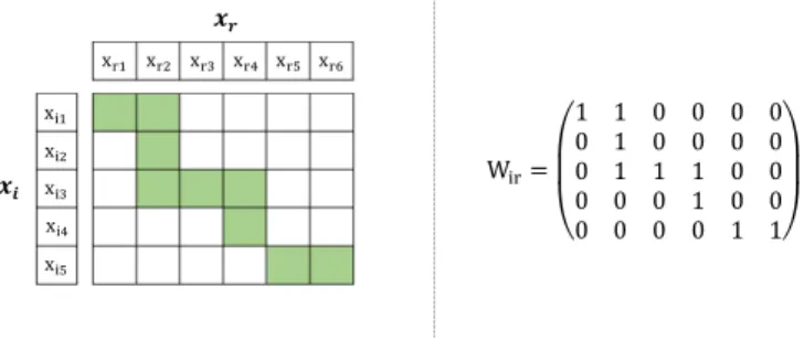
351 ⇡⇤ = arg min ⇡=(⇡1,⇡2) kx⇡1 i x ⇡2 r k2 (43) where x⇡1 i = (xi ⇡1(1), ..., xi ⇡1(m)) and x ⇡2 r = (xr ⇡2(1), ..., xr ⇡2(m)) are xi and 352 xr aligned through ⇡. 353 354

We define fr, the temporal embedding function, to embed time series xi 2

355

Rd⇥ti _{into a new temporal metric space as:}

356 fr: X ! eX⇢ eI = Rd⇥t ⇤ xi ! fr(xi) = xiWirNir (44) where Wir 2 {0, 1}ti⇥t ⇤

is the binary matrix related to the optimal

tempo-357

ral alignment between xi and xr, as shown in Figure 1 (right). The matrix

(14)

x"# W"%= ⎝ ⎜ ⎛ 1 1 0 0 0 0 0 1 0 0 0 0 0 1 1 1 0 0 0 0 0 1 0 0 0 0 0 0 1 1⎠ ⎟ ⎞ x"/ x"0 x%# x%/ 12 13 x"4 x"5 x%4 x%5 x%0 x%6

Figure 1: In the left, the temporal alignment between xi(ti= 5) and xr(t⇤= 6), the optimal

alignment ⇡⇤_{is indicated in green. In the right, the adjacency binary matrix related to the}

optimal temporal alignment.

Nir= diag(WirT1ti)

1_{is the weight diagonal matrix of order t}⇤_{, of general term}

359

1

|Nt|, that gives the weight of the element t of xr, where|Nt| is the number of

360

time stamps of xi aligned to t. In particular, note that xr remains unchanged

361

by fr, as Wrr= Nrr = diag([1, 1, . . . , 1]).

362 363

The set of embedded time series eX ={fr(x1), ..., fr(xN)} is for now lying

364

in a metric space eI, where the delays are resorbed w.r.t. the representative

365

time series xr. The pre-image solution provided in the method described in

366

Section4.1can be developed to establish a linear or nonlinear transformations

367

to preserve an isometry between eX and (X). The algorithm for the proposed

368

solution TsPrima is summarised in Algorithm 1.

369

Algorithm 1 TsPrima: Pre-image estimation for time series

1: Input: {xi}Ni=1 with xi 2 Rd⇥ti,  (a temporal kernel), b (a Gaussian

kernel),

2: (with ' =PNi=1 i (xi)), n (the neighbourhood size)

3: Output: x⇤ _{the pre-image estimation of '}

4:

5: DefineN',N'1and xr using respectively (40), (41) and (42)

6: EmbedN 1

' into a temporal metric space by using Eq. (44), set eN'1 =

fr(N'1)

7: Set X = eN 1

' and (X) =N'

8: Learn a linear (resp. nonlinear) transformation R by using Eq. (31) (resp.

Eq. (35))

9: Estimate the pre-image x⇤ _{based on a linear (resp. nonlinear)}

(15)

5. Experiments

370

In this section, we evaluate the efficiency of the proposed pre-image

esti-371

mation method under three major time series analysis tasks: 1) time series

372

averaging, 2) time series reconstruction and denoising and 3) time series

rep-373

resentation learning. The proposed pre-image estimation method TsPrima is

374

compared to three major alternative approaches introduced in Section 3, and

375

referenced in the following as Honeine, Kwok and Bakir methods. The

exper-376

iments are conducted on 33 public datasets (Table1) including univariate and

377

multivariate time series data, that may involve varying delays and be of the

378

same or di↵erent lengths. The 25 first datasets in Table1are selected from the

379

archive given in [8, 11] by using three selection criteria: a) have a reasonable

380

number of classes (Nb. of Classes < 50), b) have a sufficient size for train and

381

test samples (Train size <= 500 and Test size < 3000), c) avoid time series of

382

extra large lengths (Time series length < 700). To obtain a manageable number

383

of datasets, the 3 above selection criteria are applied on the top 40 datasets, in

384

the order set out in [8]. The 25 obtained datasets are composed of univariate

385

time series and half of the datasets include significant delays. We consider a

386

dataset as including significant delays if the di↵erence between the 1-NN

Eu-387

clidean distance error and the 1-NN Dynamic time warping [21] error is greater

388

than 5%. The 5 next datasets include univariate and multivariate time series

389

covering local and noisy salient events as described in [30,27,14] and the three

390

last datasets are related to handwritten digits and characters, they are described

391

as multivariate time series of variable lengths [7]. In the following, we detail the

392

evaluation process of the pre-image estimation methods then give and discuss

393

the obtained results.

394

5.1. Time series averaging

395

Estimating the centroid of a set of time series is a major topic for many time

396

series analytics as summarisation, prototype extraction or clustering. Time

se-397

ries averaging has been an active area in the last decade, where the propositions

398

mainly focus on tackling the tricky problem of multiple temporal alignments

399

[14, 26, 27]. A suitable way to circumvent the problem of multiple temporal

400

alignments is to use a temporal kernel method to evaluate the time series

cen-401

troid in the feature space. The pre-image of the centroid is then estimated to

402

obtain the time series averaging in the input space.

403 404

In that context, let {xi}Ni=1 and { (xi)}Ni=1 be, respectively, a set of time

405

series and their mapped images into the Hilbert spaceH related to the temporal

406

kernel dtak [25]. Let ' = _N1 PNi=1 (xi) be the centroid of the mapped time

407

series in the feature space and x⇤_{its pre-image in the input space. The quality}

408

of the obtained centroids is given by the within-class similarityP_idtak(x⇤_{, x}

i);

409

the higher the within-class similarity, the better is the estimated centroid.

410 411

To evaluate the efficiency of each pre-image estimation method, the time

412

series centroid is estimated for each class of the studied datasets and the induced

(16)

Table 1: Data Description

Dataset Nb. Classes Train Test Time series Univariate

size size length

CC 6 300 300 60 X GunPoint 2 50 150 150 X CBF 3 30 900 128 X OSULeaf 6 200 242 427 X SwedishLeaf 15 500 625 128 X Trace 4 100 100 275 X FaceFour 4 24 88 350 X Lighting2 2 60 61 637 X Lighting7 7 70 73 319 X ECG200 2 100 100 96 X Adiac 37 390 391 176 X FISH 7 175 175 463 X Beef 5 30 30 470 X Co↵ee 2 28 28 286 X OliveOil 4 30 30 570 X DiatomSizeR 4 16 306 345 X ECG5Days 2 23 861 136 X FacesUCR 14 200 2050 131 X ItalyPowerD 2 67 1029 24 X MedicalImages 10 381 760 99 X MoteStrain 2 20 1252 84 X SonyAIBOII 2 27 953 65 X SonyAIBO 2 20 601 70 X Symbols 6 25 995 398 X TwoLeadECG 2 23 1139 82 X spiral1 1 50 50 101 7 spiral2 1 50 50 300 7 PowerCons 2 73 292 144 X BME 3 30 150 128 X UMD 3 36 144 150 X digits 10 100 100 29⇠218 7 lower 26 130 260 27⇠163 7 upper 26 130 260 27⇠412 7

within-class similarity is evaluated. The average within-class similarity is then

414

reported in Table2for each dataset and each pre-image estimation method; the

415

best values are indicated in bold (t-test at 5% risk). In addition, a Nemenyi

416

test [12] is performed to compare the significance of the obtained results, with

417

the related critical di↵erence diagram given in Figure 2. The estimated time

418

series centroids for some challenging classes are shown in Figure 3, where we

419

retain particularly spiral1 and the handwritten digits and characters datasets

(17)

(digits, lower and upper) as they are more intuitive to visually evaluate the

421

quality of the estimated time series centroids.

422

Table 2: Average within-class similarity of the estimated time series centroids

DataSet TsPrima Honeine Kwok Bakir

CC 0.744 0.709 0.721 0.709 GunPoint 0.902 0.910 0.882 0.886 CBF 0.798 0.737 0.755 0.737 OSULeaf 0.985 0.987 0.986 0.987 SwedishLeaf 0.910 0.920 0.920 0.920 Trace 0.998 0.992 0.991 0.992 FaceFour 0.981 0.980 0.981 0.98 Lighting2 0.918 0.876 0.859 0.875 Lighting7 0.964 0.930 0.930 0.931 ECG200 0.593 0.565 0.567 0.566 Adiac 0.997 0.997 0.996 0.997 FISH 0.996 0.995 0.994 0.995 Beef 0.900 0.892 0.898 0.890 Co↵ee 0.998 0.998 0.998 0.998 OliveOil 0.999 0.999 0.998 0.999 DiatomSizeR 0.997 0.997 0.997 0.997 ECG5Days 0.777 0.746 0.417 0.746 FacesUCR 0.721 0.699 0.648 0.700 ItalyPowerD 0.610 0.552 0.420 0.542 MedicalImages 0.671 0.644 0.637 0.646 MoteStrain 0.776 0.777 0.701 0.777 SonyAIBOII 0.749 0.740 0.716 0.740 SonyAIBO 0.960 0.962 0.955 0.962 Symbols 0.959 0.949 0.904 0.951 TwoLeadECG 0.980 0.977 0.911 0.977 spiral1 0.831 0.823 0.799 0.824 spiral2 0.947 0.940 0.934 0.940 PowerCons 0.458 0.328 0.436 0.330 BME 0.701 0.572 0.638 0.555 UMD 0.800 0.765 0.724 0.755 digits 0.746 0.575 0.657 0.581 lower 0.713 0.544 0.645 0.545 upper 0.764 0.572 0.570 0.573 Nb. Best 28 9 4 8 Avg. Rank 1.5 2.68 3.24 2.58

5.2. Time series reconstruction and denoising

423

The reconstruction and denoising tasks represent a standard application

con-424

text for pre-image estimation. For the time series reconstruction task, a kernel

(18)

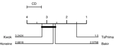
CD 4 3 2 1 1.5 TsPrima 2.5758 Bakir 2.6818 Honeine 3.2424 Kwok

Figure 2: Nemenyi test: comparison of pre-image methods under centroid estimation task

PCA is performed on the training set, the reconstruction of a given test sample

426

x is then defined as the pre-image x⇤ of its kernel PCA projection P ( (x)).

427

The latter takes the form ' = (X) , with defined as:

428

= (IN 1N) ↵ ↵Tke

T

x +N11N (45)

The quality of the reconstruction is then measured as the similarity dtak(x⇤_{, x)}

429

between each test sample x and its reconstruction x⇤; the higher the criterion,

430

the better is the reconstruction. Table 3 gives the average quality of

recon-431

struction obtained for each dataset and each method. Figure4gives the critical

432

di↵erence diagram related to the Nemenyi test for the average ranking

compar-433

ison of the studied methods. Figure 5 shows the reconstructions obtained for

434

some challenging time series of digits, lower and upper datasets.

435 436

For the time series denoising task, first a kernel PCA is performed on the

437

training set, then a (0, 2_{) Gaussian noise is added to the test samples x to}

438

generate noisy samples ˜x with di↵erent variances 2_{. The denoised sample is}

439

obtained as the pre-image x⇤ _{of its kernel PCA projection P ( (˜}_{x)), with}

440

defined as in Eq. (45). Similarly, the quality of the denoising is measured as the

441

similarity dtak(x⇤_{, x) between x}⇤_{and the initial x. Table}₄_{gives, for di↵erent}

442

values of 2_{, the average quality of the denoising for some datasets. Figure}₆

443

illustrates the denoising results for some challenging times series of the noisy

444

spiral2 data and of the class “M” of upper dataset.

(19)

Figure 3: Time series centroids for some challenging classes of digits, lower, upper and spiral1 datasets

(20)

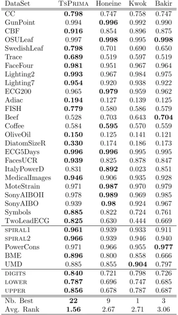
Table 3: Quality of the time series reconstruction under kernel PCA

(21)

CD 4 3 2 1 1.5606 TsPrima 2.6667 Honeine 2.7121 Kwok 3.0606 Bakir

Figure 4: Nemenyi test: comparison of pre-image methods under kernel PCA reconstruction

Figure 5: The time series reconstruction under kernel PCA of some samples of digits, lower and upper datasets

(22)

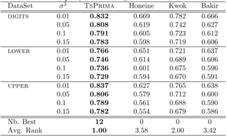
Table 4: Quality of the denoising for several noise levels

DataSet 2 _TsPrima _Honeine _Kwok _Bakir

digits 0.01 0.832 0.669 0.782 0.666 0.05 0.808 0.619 0.742 0.627 0.1 0.791 0.605 0.723 0.612 0.15 0.783 0.598 0.719 0.606 lower 0.01 0.766 0.651 0.721 0.637 0.05 0.746 0.614 0.689 0.606 0.1 0.736 0.601 0.675 0.596 0.15 0.729 0.594 0.670 0.591 upper 0.01 0.837 0.627 0.765 0.638 0.05 0.806 0.579 0.712 0.600 0.1 0.789 0.561 0.688 0.590 0.15 0.782 0.554 0.679 0.586 Nb. Best 12 0 0 0 Avg. Rank 1.00 3.58 2.00 3.42

(23)

Figure 6: Time series denoising under kernel PCA of noisy samples of spiral2 and of the class “M” of upper dataset.

(24)

5.3. Time series representation learning

446

For time series representation learning, the kernel k-SVD (⌧ = 5) is used

447

to learn, for each class of the considered datasets, the dictionary (X)B and

448

the sparse representations A = [a1, ..., aN] of its membership time series, as

449

defined in Section2.2. The pre-images D⇤and X⇤of the dictionary (X)B and

450

of the sparse codes A are then obtained by considering = B and = BA,

451

respectively. The quality of the learned sparse representations is then measured

452

as the similarity dtak(xi, x⇤i) between each time series xi and the pre-image

453

x⇤

i of the sparse representation (X)B ai. Table 5 gives the average quality

454

of the learned representations for each dataset and each pre-image estimation

455

method. Figure 7gives the critical di↵erence diagram related to the Nemenyi

456

test for the average ranking comparison of the studied methods. Figure8shows

457

the learned representations for some time series of digits, lower and upper

458

datasets and Figure 9 illustrates, for a challenging sample of the class “k” of

459

lower dataset, the learned representations as well as the top 3 atoms involved

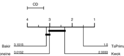
460 in its reconstruction. 461 CD 4 3 2 1 1.5 _TsPrima 2.3333 _Kwok 3.0152 Honeine 3.1515 Bakir

Figure 7: Nemenyi test: comparison of pre-image methods under kernel k-SVD representation learning

(25)

Table 5: Quality of the time series representation learning under Kernel k-SVD

(26)

Figure 8: The learned time series representations under kernel k-SVD of some samples of digits, lower, upper datasets

(27)

Figure 9: The sparse representation of a time series of the class “k” of lower dataset and the top 3 involved atoms for its reconstruction

(28)

5.4. Further comparison

462

In the previous experiments (Sections 5.1 to 5.3), we have evaluated the

463

performances of TsPrima that are mainly due to two major ingredients : 1)

464

the defined temporal embedding function fr (Section4.2) and 2) the proposed

465

transformation R to preserve an isometry between the time series embedding

466

space and the feature space (Section4.1). In this last part, the aim is to evaluate

467

the efficiency of the proposed transformation R, regardless of the e↵ect of fr.

468

For that, TsPrima is compared to the alternative methods Honeine, Kwok and

469

Bakir once all the time series embedded into the same metric space; namely,

470

all the pre-image estimation methods are performed between the time series

471

embedding space and the feature space. Similar experiments are performed on

472

the 33 public datasets (Table 1), the results obtained for the three tasks are

473

summarised into Table6and the related Nemenyi tests are given in Figure10.

474

Table 6: Further comparisons for pre-image estimation

TsPrima Honeine Kwok Bakir

Averaging Nb. Best 19 20 4 19

Avg. Rank 2.23 2.21 3.35 2.21

Reconstruction Nb. Best 24 10 0 1

(kernel PCA) Avg. Rank 1.56 2.35 3.05 3.05

Denoising Nb. Best 12 0 0 0

(kernel PCA) Avg. Rank 1.50 3.25 2.62 3.12

Rep. Learning Nb. Best 25 8 1 2

(kernel kSVD) Avg. Rank 1.44 2.67 2.58 3.32

CD 4 3 2 1 2.2121_Honeine 2.2121_Bakir 2.2273 TsPrima 3.3485 Kwok (a) Averaging CD 4 3 2 1 1.5606 _TsPrima 2.3485 _Honeine 3.0455 Kwok 3.0455 Bakir

(b) Reconstruction (kernel PCA)

CD 4 3 2 1 1 _TsPrima 2.625 _Kwok 3.125 Bakir 3.25 Honeine

(c) Denoising (kernel PCA)

CD 4 3 2 1 1.4394_TsPrima 2.5758_Kwok 2.6667 Honeine 3.3182 Bakir (d) Reconstruction (kernel k-SVD) Figure 10: Nemenyi Tests.

(29)

5.5. Overall analysis

475

The experiments conducted in Sections 5.1to 5.3 show that the proposed

476

method TsPrima leads on almost all the datasets and through the three

stud-477

ied tasks to the best results. On the other hand, the performances obtained by

478

the alternative methods seem slightly equivalent and lower than those obtained

479

by TsPrima.

480 481

In particular, for time series averaging task, we can see in Table2that the

482

centroids estimated by TsPrima lead to the highest within-class similarity on

483

almost all the datasets; namely, each centroid obtained by TsPrima is in

gen-484

eral the closest to the set of time series it represents. The analysis of the critical

485

di↵erence diagram given in Figure2indicates that the next best results are

ob-486

tained respectively by Bakir, Honeine and Kwok methods. In addition, as the

487

state of the art methods are connected by a solid bold line, their performances

488

remain equivalent. From Figure3, we can see that while all the methods succeed

489

to restitute the centroids of some input classes (shown on the left column) as

490

the class ”6” of digits and ”S” of upper dataset, only TsPrima succeeds to

491

estimate the centroids of the most challenging classes, as the ”k” class of lower

492

dataset and spiral1.

493 494

For time series reconstruction, Table 3 shows that TsPrima leads to the

495

highest reconstruction accuracies through almost all the datasets, followed by

496

Honeine, Bakir and Kwok methods. Figure 4indicates that there is no

signifi-497

cant di↵erence between the performances of the three state of the art methods

498

(connected by a solid bold line). These results are assessed in Figure 5 that

499

shows, for some input time series, the quality of the reconstructions obtained

500

by TsPrima and the state of the art methods.

501 502

For the time series denoising task, we observe from Table4 and for all the

503

methods that the quality of the denoising decreases when the intensity of noise

504

increases. This result is illustrated in Figure6, that shows the denoising results

505

of the time series ”M” of upper dataset and of the highly noisy time series of

506

spiral2 dataset. In particular, note that that Kwok and TsPrima methods

507

lead to the best results on spiral2 data and seem less sensitive to noise than

508

Honeine and Bakir methods.

509 510

Lastly, for time series representation learning task, Table 5 indicates that

511

each studied method leads to the best sparse representations for at least some

512

datatsets and that TsPrima performs better on almost all the datasets.

Fig-513

ure8shows the goodness of the sparse representations obtained. While all the

514

methods succeed to sparse represent some input time series, the time series of

515

”k” and ”B” classes appear challenging for Honeine and Bakir methods. In

Fig-516

ure9, we get a look on the quality of the learned atoms, that are involved into

517

the reconstruction of the input samples. The first row gives for some input

sam-518

ple ”k” (on the left), the sparse representations learned by each method. The

(30)

three next rows, provide the three first atoms involved into the reconstructions.

520

We can see that while the first atom learned by TsPrima is nearly sufficient

521

to sparse represent the ”k” input sample, the state of the art methods need

522

obviously more that one atom to sparse represent the input sample. Finally,

523

the analysis of Figure 7 indicates that Honeine method performs equivalently

524

than Kwok and Bakir, whereas the Kwok performances are significantly better

525

that those of Bakir method.

526 527

Further comparisons (Table6) are conducted in Section5.4to evaluate the

528

efficiency of TsPrima related to the learned transformation R, regardless of

529

the temporal embedding fr. For averaging task, TsPrima, Honeine and Bakir

530

lead equivalently to the best performances, followed by Kwok method (Figure

531

10(a)). From these results we can conjecture that, linear transformations seem

532

sufficient to achieve good pre-image estimations for averaging task on these

533

datasets, as both linear and non linear approaches (TsPrima, Honeine, Bakir)

534

perform equivalently. Furthermore, while Honeine and Bakir involve the whole

535

datasets for the centroid pre-image estimations, Kwok uses a subset of samples

536

into the neighbourhood of ', which may explain the slightly lower performances

537

of Kwok method. Note that, although TsPrima involves, similarly to Kwok

538

method, fewer samples into the neighbourhood of ', it succeeds to reach the

539

best performances thanks to the efficiency of the learned transformation R.

540

For the remaining tasks reconstruction, denoising and representation learning,

541

TsPrima achieves the highest performances, followed by far by Honeine, Kwok

542

and Bakir (Figure 10(b), (c) and (d)), which assesses the crucial contribution

543

of the learned transformations R of TsPrima. Lastly, of particular note is that

544

Honeine and Bakir that involve the whole training samples induce much

com-545

putations, specifically for the time series embedding process, than Kwok and

546

TsPrima that require fewer samples into the neighbourhood of '.

547 548

Finally, as all the studied methods propose closed-form solutions, they lead

549

to comparable complexities. However, for large data, TsPrima and Kwok

meth-550

ods are expected to perform faster as requiring fewer samples on the

neighbor-551

hood of ' than Honeine and Bakir that involve the whole samples for pre-image

552

estimation. Note that the complexity of the proposed solutions is mainly

re-553

lated to the matrix inversion operator. In Kwok method, the inversion of ZZT

554

required in Eq. (21), with Z of dimension (q⇥ n) and n is the neighbourhood

555

size, induces a complexity of O(q2_{n) + O(q}3_{); as q is in general small and fixed}

556

beforehand, the overall complexity is about O(n). For Honeine method, Eq.

557

(24) requires two inversions of XXT _{and K, which induces, respectively, a}

com-558

plexity of O(d2_{N ) + O(d}3_{) and O(N}3_{), that leads to an overall complexity of}

559

O(N3_{). For Bakir method, Eq. (}₂₆_{), requires the inversion of the Gram matrix,}

560

which leads to a complexity of O(N3_{). For TsPrima, Eq. (}₃₂_{) involves the}

561

inversion of XXT_{, with X is of dimension (d}_{⇥ n), d is the time series length}

562

and n is the neighbourhood size. The induced complexity is of O(d2_{n) + O(d}3_).

563

For the time series embedding part, the complexity is mainly related to the

564

time warping function which is of order O(d2_{n). As d is in general higher that}

(31)

the neighbourhood size n, the overall complexity for TSPrima is about O(d3_).

566

To sum up, as the neighbourhood size n << N and d << N (for not extra

567

large time series), the complexity induced by both Kwok and TSPrima remains

568

lower that the one of Honeine and Bakir. Note that, the Honeine method can

569

be developed to consider only the neighbourhoods instead of all samples.

570

6. Conclusion

571

This work proposes TsPrima, a new closed-form pre-image estimation method

572

for time series analytics under kernel machinery. The method consists of two

573

stages. In the first step, we define a time warp embedding function, driven by

574

distance constraints in the feature space, that allows to embed the time series in

575

a metric space. In the second step, the time series pre-image estimation is cast

576

as learning a linear (or a nonlinear) transformation to ensure a local isometry

577

between the time series embedding space and the feature space. Extensive

ex-578

periments show the efficiency and the benefits of TsPrima through three major

579

tasks that require pre-image estimation: 1) time series averaging, 2) time series

580

reconstruction and denoising and 3) time series representation and dictionary

581

learning. Future work will focus on using pre-image estimation methods to

en-582

hance the interpretability and the computation of deep learning tasks for time

583

series, sequence and graph analytics.

584

Acknowledgment

585

This work is supported by the French National Research Agency through

586

the projects locust (ANR-15-CE23-0027-02) and APi (ANR-18-CE23-0014).

587

References

588

[1] Aharon, M., Elad, M., Bruckstein, A., 2006. K-svd: An algorithm for

589

designing overcomplete dictionaries for sparse representation. IEEE

Trans-590

actions on signal processing 54, 4311–4322.

591

[2] Bahlmann, C., Haasdonk, B., Burkhardt, H., 2002. Online handwriting

592

recognition with support vector machines-a kernel approach, in:

Proceed-593

ings Eighth International Workshop on Frontiers in Handwriting

Recogni-594

tion, IEEE. pp. 49–54.

595

[3] Bakır, G.H., Weston, J., Sch¨olkopf, B., 2004. Learning to find pre-images.

596

Advances in neural information processing systems 16, 449–456.

597

[4] Balasubramanian, K., Yu, K., Lebanon, G., 2013. Smooth sparse coding

598

via marginal regression for learning sparse representations, in: International

599

Conference on Machine Learning, pp. 289–297.

600

[5] Bengio, S., Pereira, F., Singer, Y., Strelow, D., 2009. Group sparse coding,

601

in: Advances in neural information processing systems, pp. 82–89.

(32)

[6] Bianchi, F.M., Livi, L., Mikalsen, K.Ø., Kamp↵meyer, M., Jenssen,

603

R., 2018. Learning representations for multivariate time series with

604

missing data using temporal kernelized autoencoders. arXiv preprint

605

arXiv:1805.03473 .

606

[7] Chen, M., AlRegib, G., Juang, B.H., 2012. 6dmg: A new 6d motion

ges-607

ture database, in: Proceedings of the 3rd Multimedia Systems Conference,

608

ACM. pp. 83–88.

609

[8] Chen, Y., Keogh, E., Hu, B., Begum, N., Bagnall, A., Mueen, A., Batista,

610

G., 2015. The ucr time series classification archive URL:https://www.cs.

611

ucr.edu/~eamonn/time_series_data/.

612

[9] Cloninger, A., Czaja, W., Doster, T., 2017. The pre-image problem for

613

laplacian eigenmaps utilizing l 1 regularization with applications to data

614

fusion. Inverse Problems 33, 074006.

615

[10] Cuturi, M., Vert, J.P., Birkenes, O., Matsui, T., 2007. A kernel for time

616

series based on global alignments, in: 2007 IEEE International Conference

617

on Acoustics, Speech and Signal Processing-ICASSP’07, IEEE. pp. II–413.

618

[11] Dau, H.A., Keogh, E., Kamgar, K., Yeh, C.C.M., Zhu, Y., Gharghabi, S.,

619

Ratanamahatana, C.A., Yanping, Hu, B., Begum, N., Bagnall, A., Mueen,

620

A., Batista, G., Hexagon-ML, 2018. The ucr time series classification

621

archive. https://www.cs.ucr.edu/~eamonn/time_series_data_2018/.

622

[12] Demˇsar, J., 2006. Statistical comparisons of classifiers over multiple data

623

sets. Journal of Machine learning research 7, 1–30.

624

[13] Do, C.T., Douzal-Chouakria, A., Mari´e, S., Rombaut, M., Varasteh, S.,

625

2017. Multi-modal and multi-scale temporal metric learning for a robust

626

time series nearest neighbors classification. Information Sciences 418, 272–

627

285.

628

[14] Frambourg, C., Douzal-Chouakria, A., Gaussier, E., 2013. Learning

multi-629

ple temporal matching for time series classification, in: International

Sym-630

posium on Intelligent Data Analysis, Springer. pp. 198–209.

631

[15] Honeine, P., Richard, C., 2011a. A closed-form solution for the pre-image

632

problem in kernel-based machines. Journal of Signal Processing Systems

633

65, 289 – 299. URL: https://link.springer.com/article/10.1007/

634

s11265-010-0482-9, doi:10.1007/s11265-010-0482-9.

635

[16] Honeine, P., Richard, C., 2011b. Preimage problem in kernel-based

636

machine learning. IEEE Signal Processing Magazine 28, 77 – 88.

637

URL: https://ieeexplore.ieee.org/document/5714388, doi:10.1109/

638

MSP.2010.939747.

639

[17] Jenatton, R., Mairal, J., Obozinski, G., Bach, F.R., 2010. Proximal

meth-640

ods for sparse hierarchical dictionary learning., in: ICML, Citeseer. p. 2.

(33)

[18] Kwok, J.Y., Tsang, I.H., 2004. The pre-image problem in kernel methods.

642

IEEE transactions on neural networks 15, 1517–1525.

643

[19] Paparrizos, J., Franklin, M.J., 2019. Grail: efficient time-series

representa-644

tion learning. Proceedings of the VLDB Endowment 12, 1762–1777.

645

[20] Pati, Y.C., Rezaiifar, R., Krishnaprasad, P.S., 1993. Orthogonal matching

646

pursuit: Recursive function approximation with applications to wavelet

647

decomposition, in: Proceedings of 27th Asilomar conference on signals,

648

systems and computers, IEEE. pp. 40–44.

649

[21] Sakoe, H., Chiba, S., 1978. Dynamic programming algorithm optimization

650

for spoken word recognition. IEEE transactions on acoustics, speech, and

651

signal processing 26, 43–49.

652

[22] Schlegel, K., 2019. When is there a representer theorem? Journal of Global

653

Optimization 74, 401–415. doi:10.1007/s10898-019-00767-0.

654

[23] Schölkopf, B., Mika, S., Smola, A., Rätsch, G., Müller, K.R., 1998. Kernel

655

pca pattern reconstruction via approximate pre-images, in: International

656

Conference on Artificial Neural Networks, Springer. pp. 147–152.

657

[24] Scholkopf, B., Smola, A.J., 2001. Learning with kernels: support vector

658

machines, regularization, optimization, and beyond. MIT press.

659

[25] Shimodaira, H., Noma, K.i., Nakai, M., Sagayama, S., 2002. Dynamic

660

time-alignment kernel in support vector machine, in: Advances in neural

661

information processing systems, pp. 921–928.

662

[26] Soheily-Khah, S., Chouakria, A.D., Gaussier, E., 2015. Progressive and

it-663

erative approaches for time series averaging., in: AALTD@ PKDD/ECML.

664

[27] Soheily-Khah, S., Douzal-Chouakria, A., Gaussier, E., 2016. Generalized

665

k-means-based clustering for temporal data under weighted and kernel time

666

warp. Pattern Recognition Letters 75, 63–69.

667

[28] Van Nguyen, H., Patel, V.M., Nasrabadi, N.M., Chellappa, R., 2012. Kernel

668

dictionary learning, in: 2012 IEEE International Conference on Acoustics,

669

Speech and Signal Processing (ICASSP), IEEE. pp. 2021–2024.

670

[29] Wu, L., Yen, I.E.H., Yi, J., Xu, F., Lei, Q., Witbrock, M., 2018. Random

671

warping series: A random features method for time-series embedding. arXiv

672

preprint arXiv:1809.05259 .

673

[30] Yazdi, S.V., Douzal-Chouakria, A., 2018. Time warp invariant ksvd: Sparse

674

coding and dictionary learning for time series under time warp. Pattern

675

Recognition Letters 112, 1–8.

(34)

[31] Yazdi, S.V., Douzal-Chouakria, A., Gallinari, P., Moussallam, M., 2018.

677

Time warp invariant dictionary learning for time series clustering:

appli-678

cation to music data stream analysis, in: Joint European Conference on

679

Machine Learning and Knowledge Discovery in Databases, Springer. pp.

680

356–372.

681

[32] Zhu, F., Honeine, P., 2016. Bi-objective nonnegative matrix factorization:

682

Linear versus kernel-based models. IEEE Transactions on Geoscience and

683

Remote Sensing 54, 4012 – 4022. URL:https://ieeexplore.ieee.org/

684

document/7448928, doi:10.1109/TGRS.2016.2535298.