HAL Id: inserm-00589183
https://www.hal.inserm.fr/inserm-00589183
Submitted on 29 Apr 2011
HAL is a multi-disciplinary open access
archive for the deposit and dissemination of
sci-entific research documents, whether they are
pub-lished or not. The documents may come from
teaching and research institutions in France or
abroad, or from public or private research centers.
L’archive ouverte pluridisciplinaire HAL, est
destinée au dépôt et à la diffusion de documents
scientifiques de niveau recherche, publiés ou non,
émanant des établissements d’enseignement et de
recherche français ou étrangers, des laboratoires
publics ou privés.
Mapping the distance between the brain and the inner
surface of the skull and their global asymmetries
Marc Fournier, Benoît Combès, Neil Roberts, José Braga, Sylvain Prima
To cite this version:
Marc Fournier, Benoît Combès, Neil Roberts, José Braga, Sylvain Prima. Mapping the distance
between the brain and the inner surface of the skull and their global asymmetries. Medical Imaging
2011: Image Processing, Feb 2011, Orlando, United States. pp.79620Y, �10.1117/12.876795�.
�inserm-00589183�
Mapping the distance between the brain and the inner surface
of the skull and their global asymmetries
Marc Fournier
1, Benoît Combès
1, Neil Roberts
2, José Braga
3, Sylvain Prima
11
INSERM, IRISA-INRIA VisAGeS Project-Team, F-35042 Rennes, France
2CRIC, Queen’s Medical Research Institute, Edinburgh, U.K.
3
AMIS, Paul Sabatier University, Toulouse, France
ABSTRACT
The primary goal of this paper is to describe i) the pattern of pointwise distances between the human brain (pial surface) and the inner surface of the skull (endocast) and ii) the pattern of pointwise bilateral asymmetries of these two structures. We use a database of MR images to segment meshes representing the outer surface of the brain and the endocast. We propose automated computational techniques to assess the endocast-to-brain distances and endocast-and-brain asymmetries, based on a simplified yet accurate representation of the brain surface, that we call the brain hull. We compute two meshes representing the mean endocast and the mean brain hull to assess the two patterns in a population of normal controls. The results show i) a pattern of endocast-to-brain distances which are symmetrically distributed with respect to the mid-sagittal plane and ii) a pattern of global endocast and brain hull asymmetries which are consistent with the well-known Yakovlevian torque. Our study is a first step to validate the endocranial surface as a surrogate for the brain in fossil studies, where a key question is to elucidate the evolutionary origins of the brain torque. It also offers some insights into the normal configuration of the brain/skull interface, which could be useful in medical imaging studies (e.g. understanding atrophy in neurodegenerative diseases or modeling the brain shift in neurosurgery).
Keywords: Brain-skull MRI segmentation; Brain-skull relations; Surface-based brain hull; Brain-endocast distance;
Brain asymmetry; Endocranial asymmetry; Average brain-endocast shapes; Brain-endocast asymmetry t-test.
1. INTRODUCTION
The human brain has been often reported to exhibit a global, counterclockwise, so-called Yakovlevian, torque1 about a
vertical axis (i.e. parallel to the long axis of the human body). The magnitude of this torque has been quantified variously in terms of the i) greater widths or volumes, or ii) anterior and posterior protrusion of the brain in the right as compared to the left frontal lobe and in the left compared to the right occipital lobe or iii) leftward (resp. rightward) deviation of the inter-hemispheric fissure between the frontal (resp. occipital) lobes. Measuring the torque is of the utmost importance, as it has often been hypothesized to be the neural substrate for cerebral hemisphere dominance for language in humans. As of today, it is not clear i) when this pattern appeared during the course of human evolution and ii) whether this pattern is shared by other species, and especially by our closest extant relatives (bonobos and chimpanzees). The first question is typically addressed by physical anthropologists, using CT imaging of fossil skulls and segmentation of the inner surface of the skull to obtain a so-called virtual endocast2. The second question can be addressed using MR imaging of the brain and segmentation of the outer cortical surface of the brain3. However, both approaches led to controversial results. First, it is not clear whether the endocast is a faithful surrogate representation of the brain as it is separated from it by the dura mater, the pia mater and the arachnoid (blood vessels, CSF); these layers are of varying thickness between anatomical regions. Second, local intra-subject (i.e. differences between hemispheres) and inter-subject sulcogyral variability makes it difficult to assess the torque, which is a global pattern.
In this paper, we propose to address these two questions using MRI by i) measuring the local distances between the brain and the endocast and ii) measuring the asymmetries of the brain and of the endocast. To alleviate the problems due to cortical variability, we base our measures on a simplified yet accurate representation of the brain (that we call the brain hull) which closely follows the gyri without entering the sulci. Both the brain hull and the endocast are represented by 3D meshes. In the first study, using a dataset of 37 healthy control subjects, we compute individual pointwise endocast-to-brain distances, and we map them onto a mean endocast computed from the population. In the second study, using a subset of 14 right-handed males, we compute individual pointwise asymmetry maps of endocast and brain hull
separately, and we map them onto, respectively, a mean endocast and mean brain hull computed from the subpopulation. Student's t-test is used to assess statistically significant brain and endocranial asymmetries. The results show i) a pattern of endocast-to-brain distances which are symmetrically distributed with respect to the mid-sagittal plane and ii) a pattern of global endocast and brain hull asymmetries which are consistent with the well-known Yakovlevian torque. The first pattern of distances gives an insight into the normal spatial brain-skull configuration which can be useful in medical imaging applications such as brain shift modeling for neurosurgery4 or the study of brain atrophy which occurs in
pathologies such as Alzheimer’s disease5 and multiple sclerosis6. Section 2 of this paper describes the material and
methods while in Section 3 we provide and discuss some results, before concluding in Section 4.
2. MATERIAL AND METHODS
2.1 Material
In this paper we use a database of MR images of 37 healthy human subjects (25 to 45 years old) including 19 males and 18 females. The data were acquired at the MARIARC, University of Liverpool (http://www.liv.ac.uk/mariarc), using a MPRAGE T1-weighted sequence with a 3T Siemens Trio, CP Head Coil MRI scanner. The in-plane resolution is 0.625x0.625mm with a data matrix size of 320x320. The whole scan is composed of 192 slices with a thickness of 1.0mm per slice.
2.2 Brain and endocast segmentation
The first step of our method is to extract the brain and endocranial surfaces from the MR images. We use BrainMask7 to
process the MR images in order to correct the intensity non-uniformity, find the white matter seed and output the binary mask of the whole brain without hemisphere split. This software was chosen for its fully automatic pipeline process and for the quality of its segmentation results. We use FSL8 to process the MR images in order to find and output the binary
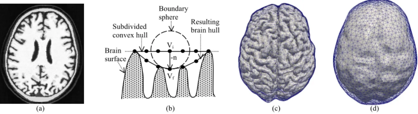
mask of the skull. We found that only a few computer programs can extract the skull from MR images, and FSL provides satisfying results for our application. Then the marching cube9 isosurface extraction algorithm is applied to both binary volume masks in order to generate mesh surfaces of the brain and endocast. Figure 1(a) shows an example of this volume segmentation preprocessing step.
2.3 Brain hull computation
The second step of our method consists in computing the brain hull from the detailed brain mesh. We first compute the 3D convex hull of the brain mesh vertices (http://www.qhull.org)10. This algorithm generates a mesh with few large triangles corresponding to a coarse representation of the brain which is not sufficiently accurate for our purpose. We subdivide this mesh to obtain a uniform triangulation with enough vertices to accurately describe the initial brain mesh gyri positions. Then for each vertex of the subdivided convex hull, we compute the minimal sphere centered on this vertex which intersects the boundary of the initial detailed brain mesh. Finally we move the vertex in its opposite normal direction (towards the brain surface) on the minimal sphere surface. This procedure illustrated in Figure 1(b) attracts vertices to the gyri positions and prevents them to penetrate inside the sulci, between neighboring gyri. It produces an accurate brain hull shown in Figure 1(c) and 1(d) with respectively the brain surface and the endocranial mesh. The brain hull represents the brain global shape, which closely follows the gyri.
Figure 1. MRI volume segmentation and mesh processing. (a) Brain and skull segmentation masks superposed on MRI
image. (b) Illustration of the brain hull computation with: Vi (resp. Vf) the initial (resp. final) vertex position of the
subdivided convex (resp. brain) hull; -n the opposite normal vertex displacement direction. (c) Brain hull mesh
(a) (b) (c) (d) Boundary sphere Brain surface Vi Vf -n Subdivided convex hull Resulting brain hull
superposed on the brain surface mesh obtained from the volume mask. (d) Endocranial mesh (from the volume mask) superposed on the brain hull surface.
2.4 Brain to endocast distance
In order to evaluate the distance pattern, we compute the local distance between the brain hull and endocast of each subject. For each vertex of the endocast, the distance to the brain hull surface is computed. Then we evaluate the average local distance for all subjects by computing an average endocranial shape. Endocasts of all subjects are registered using the ICP algorithm11 and the average endocranial shape is computed using a shape-based12 method which consists of a weighted average in the implicit distance transform domain of the meshes. Finally the same local weights used to evaluate the average shape are used to compute the corresponding local average distances.
2.5 Brain and endocranial asymmetries
In order to evaluate both asymmetry patterns, we compute local surface-based asymmetries separately for the brain hull and endocast of each subject. For this study we use a subsample of the database composed of the 14 right-handed male subjects among the 37 subjects. Both average asymmetry patterns are evaluated for all subjects by computing separately the average shapes of the brain hull and the endocast using the same procedure as for the average local distance pattern evaluation. Both brain and endocranial asymmetry measurements are achieved by flipping the brain surface over the mid-sagittal plane. The latter is defined as the median plane of the scanned MRI volume, whose position and orientation are defined by an automated atlas-based procedure13. The asymmetries are defined as the local distances between the
original brain surface and the flipped one. These distances are signed according to the surface normal in order to quantify the asymmetry orientation. We also perform the Student's t-test in order to locate significant asymmetries on the brain hull and the endocast.
3. RESULTS AND DISCUSSION
3.1 Brain to endocast distance
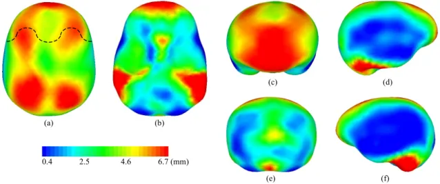
Figure 2 shows the local distance pattern between the endocast and brain hull for the dataset of 37 subjects. The average local distances are converted into a color map that is mapped onto the average endocranial shape. The distance is globally greater at the top of the brain compared to the bottom (Figures 2(a) and 2(b)). It seems that at the top of the brain the distance follows a mid (green) to high (red) values pattern in the left to right axis as illustrated by the curve in Figure 2(a). The distance is also globally greater at the front compared to the back of the brain (Figures 2(c) and 2(e)). However this observation is influenced by gravity since the subjects were scanned in supine position. Indeed relative brain-skull displacements14 are monitored under external forces such as gravity attraction. On both left and right sides of
the brain, homogenous minimal distances are observed (Figures 2(d) and 2(f)).
(c) (d) (e) (f) (a) (b) 0.4 2.5 4.6 6.7 (mm)
Figure 2. Distance color map pattern between the endocast and brain hull shown on the average endocranial mesh. (a) Top view. (b) Bottom view. (c) Front view. (d) Right side view. (e) Rear view. (f) Left side view. The linear color map scale is in millimeters and the distance values are shown on the color bar.
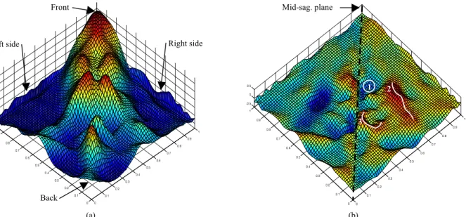
In order to better interpret this distance map pattern, we cut the underneath part (Figure 2(b) view) of the average endocranial mesh to create an open boundary mesh. We unfold this mesh onto a plane using mesh parameterization and we consider the distance pattern as a height function. We resample this distance pattern on a regular grid for display purpose and show the result in Figure 3(a) using the same color map as in Figure 2. Figure 3(a) shows all views of Figure 2 (except Figure 2(b)) embedded on the same chart using an alternative representation of the brain to endocast distance pattern. This representation displays the distance pattern in a synthetic way and suggests it is approximately symmetrical about to the mid-sagittal plane. The peaks, ridges and flatter regions are quite similar on the left and right sides of Figure 3(a). To quantify the left-right differences of this distance pattern, we compute its mirror image about the mid-sagittal plane shown in Figure 3(b) and we evaluate the local differences between the two. This symmetry difference map shown in Figure 3(b) illustrates that the three major differences (red and blue colors) are located on the peak (and its symmetrical counterpart) identified as #1 and on the two ridges (and their symmetrical counterparts) identified as #2 and #3 in Figure 3(b). Besides these three highlighted local components ranging from 0.4mm to 0.5mm, most of the other absolute differences are below 0.3mm. This observation shows that most of the symmetrical differences (< 0.3mm) are less than 5% of the maximum distance (6.7mm) between the brain and the endocast.
Figure 3. Height function of the brain to endocast distance pattern. (a) Height function of the distance pattern projected onto a plane displayed using the same color map as in Figure (2). (b) Symmetry difference of the distance pattern about the mid-sagittal plane shown using an equivalent color map scaled to the symmetrical difference data.
3.2 Brain and endocranial asymmetries
Figure 4 shows the local asymmetry patterns on the average brain hull and endocast for the data subset composed of the 14 right-handed males. Green color means there is no local asymmetry on average. Red color (versus blue color) means the original surface is “above” (resp. “below”) the surface obtained when mirroring it about the mid-sagittal plane. This can be interpreted in different ways: as a left-right difference of area, volume, width, protrusion, etc. What is noteworthy is that, for both the brain hull and the endocast, the right frontal pole is “above” the left one on average, while the opposite is observed in the occipital poles (Figures 4(a), (c), (e) and (g)). These four results are statistically significant, as shown by two t-tests on the brain hull and endocast (H0: “the pointwise asymmetry is null”, p-value = 0.05, not
corrected for multiple comparisons). The significantly asymmetrical vertices are shown in blue in Figures 4(b), (d), (f)
(a) (b)
Front
Left side Right side
Back
Mid-sag. plane
1 2
and (h). In short, it suggests that both the brain hull and the endocast exhibit the same global asymmetry pattern as the brain, i.e. the Yakovlevian torque1. The only difference is the asymmetrical regions of the endocast seem more spread
out compared to the brain hull ones according to the t-test results. The measured range of local asymmetries is the same for the brain hull and the endocast. The maximum asymmetry magnitude is also the same in both directions.
Figure 4. Asymmetry color map patterns of brain hull and endocast and their t-test shown on average shapes. (a) Brain hull front view asymmetry. (b) Brain hull front view t-test. (c) Brain hull rear view asymmetry. (d) Brain hull rear view t-test. (e) Endocast front view asymmetry. (f) Endocast front view t-test. (g) Endocast rear view asymmetry. (h) Endocast rear view t-test. The linear color map scale is in millimeters and the asymmetry values are shown on the color bar. The t-test results show significantly asymmetrical vertices (p-values lower than 0.05); green color corresponds to regions with no asymmetry and blue color to regions with asymmetry.
(a) (b) (c) (d) (e) (f) (g) (h) 3.2 1.6 0mm -1.6 -3.2 (a) (b) (c) (d) (e) (f) 2.4 1.8 1.2 0.6 0mm 0.050 0.025 0.000
Figure 5. Asymmetry differences color map between the brain and the endocast and their t-test shown on the average brain hull shape. (a) Top view of the asymmetry differences. (b) Front view of the asymmetry differences. (c) Rear view of the asymmetry differences. (d) Top view of the test result. (e) Front view of the test result. (f) Rear view of the t-test result. The asymmetry differences color map scale is in millimeters and the values are shown on the color bar. The green color on the t-test result (p-value = 0.05) corresponds to regions with no significant difference of asymmetry. The color map shows the scaling of vertices with significant differences at different confidence levels shown on the color bar.
In order to quantify the asymmetry differences between the brain hull and the endocast, we compute the local differences between both asymmetry maps. The obtained asymmetry differences map is shown for different views in Figure 5(a), 5(b) and 5(c). The front and rear views (Figure 5(b), (c)) mostly have differences near 0mm (blue color). That explains the similar Yakovlevian torque asymmetry pattern retrieved on both the brain hull and endocranial mean shapes in Figure 4. However Figure 5(a) shows approximately symmetrical regions (with respect to the mid-sagittal plane) at the top view with mid-range (green color) to larger (red color) differences. These differences are the result of larger asymmetries observed on the endocast compared to the brain hull. These differences are from 1mm (green) to 2mm (red) at the most, which is around 30% of the maximum asymmetry range. This result suggests that asymmetries in these regions measured on fossil endocasts for example should not necessarily be considered as asymmetries also belonging to the brain of extinct species. This is an interesting observation even if that region of interest is outside of the region where the typical torque is usually observed.
Figure 5 also shows t-test results (H0: “the difference between pointwise brain hull and endocranial asymmetry is null”,
p-value = 0.05, not corrected for multiple comparisons) that support the previous observations. The green color (no statistically significant difference) is observed on most of the shape including the frontal (Figure 5(e)) and occipital (Figure 5(f)) lobes where the Yakovlevian torque is observed on both the brain hull and the endocast. However the two regions with larger differences (red color on Figure 5(a)) do have more significant differences according to the t-test (light blue color on Figure 5(d)) in these two regions.
4. CONCLUSION
In this paper we presented an asymmetry and relative distance patterns study of the human brain (pial surface) and the inner table of the skull (endocast). We described preprocessing of MR images in order to extract the surfaces of interest from the volume data. We proposed a mesh processing method to obtain an accurate brain hull surface which closely follows the gyri positions without entering the neighboring sulci. This coarse representation is useful for efficient registration and average shape computation. It prevents results from being influenced by inter-subject variability in the patterns of gyri and sulci. It enables a global brain shape asymmetry mapping and comparison with the endocast. It also provides a more accurate distance mapping between the brain and endocast.
We evaluated the local distances between the endocast and brain hull and the bilateral asymmetry of both surfaces with respect to the mid-sagittal plane. Average shape meshes were computed and the distance and asymmetry patterns were projected onto these average shapes using color maps for visualization purposes. We found that our brain hull representation allows recovering the well-known global brain asymmetry (Yakovlevian torque). We also found that local distances between the endocast and brain hull follow an approximately regular and bilaterally symmetrical pattern. This explains why we also observed that the endocranial asymmetry is related to that of the brain hull.
We performed t-tests on the brain hull and endocranial asymmetries to support these findings. These results suggest that the inner surface of the skull is a relevant surrogate of brain shape, and thus that virtual endocasts can be used in paleoneurological studies to infer the evolutionary history of global brain asymmetry with respect to the Yakovlevian torque. However we also observed that a region at the top of the endocast, outside the typical torque regions, is asymmetrical in a significantly different way when compared to the brain. This suggests that this specific asymmetry, which could be observed on virtual endocasts, may not be representative of the global brain asymmetry pattern.
Future work will include other processing pipelines using different tools to validate the findings in this paper. In particular, new state-of-the-art methods to compute the mid-sagittal plane15, the asymmetries15 and the average shapes16
for both the brain hull and the endocast will be investigated. This will also involve a more extensive study over other subgroups within humans, and over other species too, such as chimpanzees that are our closest extant relatives. We will also use an available database of CT images and MR images of the same subjects to compare MR and CT-based endocasts segmentation accuracy. We will provide further quantification of the patterns of endocast-to-brain distance and endocast-and-brain asymmetries. This will involve spherical parameterization and vector field computation and
decomposition of a more specific analysis of the endocast-to-brain distance pattern. We will also design an automated comparison method between the endocast and the brain hull asymmetries including a correlation on specific anatomical regions for easier interpretation of the results.
REFERENCES
[1] Toga A., Thompson P.: Mapping brain asymmetry. Nature Reviews Neuroscience, 4(1), 37-48 (2003).
[2] Holloway R.L., De La Costelareymondie M.C.: Brain endocast asymmetry in pongids and hominids: some preliminary findings on the paleontology of cerebral dominance. American Journal of Physical Anthropology, 58(1), 101-110 (1982).
[3] Lyttelton O.C., Karama S., Ad-Dab'bagh Y., Zatorre R.J., Carbonell F., Worsley K., Evans A.C.: Positional and surface area asymmetry of the human cerebral cortex. NeuroImage, 46(4), 895-903 (2009).
[4] Miller K., Wittek A., Joldes G., Horton A., Dutta-Roy T., Berger J., Morriss L.: Modelling brain deformations for computer-integrated neurosurgery. International Journal for Numerical Methods in Biomedical Engineering, 26(1), 117-138 (2010).
[5] Fritzsche K., Wangenheim A., Dillmann R., Unterhinninghofen R.: Automated MRI-based quantification of the cerebral atrophy providing diagnostic information on mild cognitive impairment and Alzheimer's disease. IEEE Symposium on Computer-Based Medical Systems, 191-196 (2006).
[6] Losseff N.A., Wang L., Lai H.M., Yoo D.S., Gawne-Cain M.L., McDonald W.I., Miller D.H., Thompson A.J.: Progressive cerebral atrophy in multiple sclerosis A serial MRI study. Brain Journal of Neurology, 119(6), 2009-2019 (1996).
[7] Mikheev A., Nevsky G., Govindan S., Grossman R., Rusinek H.: Fully automatic segmentation of the brain from T1-weighted MRI using bridge burner algorithm. Journal of Magnetic Resonance Imaging, 27(6), 1235-1241 (2008).
[8] Smith S.M., Jenkinson M., Woolrich M.W., Beckmann C.F., Behrens T.E.J., Johansen-Berg H., Bannister P.R., Luca M., Drobnjak I., Flitney D.E., Niazy R., Saunders J., Vickers J., Zhang Y., Stefano N., Brady J.M., Matthews P.M.: Advances in functional and structural MR image analysis and implementation as FSL. NeuroImage, 23(1), 208-219 (2004).
[9] Lorensen W.E., Cline H.E.: Marching Cubes: a high resolution 3D surface reconstruction algorithm. ACM SIGGRAPH Computer Graphics, 21(4), 163-169 (1987).
[10] Barber C.B., Dobkin D.P., Huhdanpaa H.T.: The quickhull algorithm for convex hulls. ACM Transactions on Mathematical Software, 22(4), 469-483 (1996).
[11] Besl P.J., McKay N.D.: A method for registration of 3-D shapes. IEEE Transactions on Pattern Analysis and Machine Intelligence, 14(2), 239-256 (1992).
[12] Marquez Flores J., Bloch I., Schmitt F., Grangeat C., Bousquet T.: Shape-based averaging for craniofacial anthropometry. Mexican International Conference on Computer Science, 314-319 (2005).
[13] van der Kouwe A.J.W., Benner T., Fischl B., Schmitt F., Salat D.H., Harder M., Sorensen A.G., Dale A.M.: On-line automatic slice positioning for brain MR imaging. NeuroImage, 27(1), 222-230 (2005).
[14] Asiminei A.G., Depreitere B., Vander Sloten J., Verpoest I., Goffin J.: An image based approach for in vivo evaluation of the brain-skull relative displacement and brain deformation in quasi-static conditions. World Congress on Medical Physics and Biomedical Engineering, 25(4), 2185-2188 (2009).
[15] Combès B., Prima S., New algorithms to map asymmetries of 3D surfaces. Medical Image Computing and Computer Assisted Intervention, 11(Pt 1), 17-25 (2008).
[16] Combès B., Prima S., An efficient EM-ICP algorithm for symmetric consistent non-linear registration of point sets. Medical Image Computing and Computer Assisted Intervention, 13(Pt 2), 594-601 (2010).