Commitment vs. flexibility

Digitized

by

the

Internet

Archive

in

2011

with

funding

from

Boston

Library

Consortium

Member

Libraries

-, i-^k=,_VV* U.-m

31 il5

\0

Massachusetts

Institute

of

Technology

Department

of

Economics

Working

Paper

Series

COMMITMENT

vs.

FLEXIBILITY

Manuel

Amador

Ivan

Werning

George-Marios

Angeletos

Working

Paper

03-40

November]

5,

2003

Room

E52-251

50

Memorial

Drive

Cambridge,

MA

02142

Thispapercanbedownloaded withoutchargefromthe SocialScience ResearchNetworkPaperCollectionat

MASSACHUSETTS |^''T1TUTE

Commitment

vs.

Flexibility'

Manuel

Amador"'

Ivan

Werning-^

George-Marios

Angeletos^

November

15.

2003

Abstract

Thispaperstudiestheoptimaltrade-offbetween

commitment

and flexibil-ity in an intertemporal consumption/savings choice model. Indi\iduals expect to receive relevant informationregarding their

own

situation and tastes -

gen-erating a value for flexibility - _but also expect to suffer from temptations

-generating a value for commitment.

The

model combines the representations ofpreferencesforflexibihty introduced byKreps (1979) withitsrecent

antithe-sis for

commitment

proposed by Gul and Pesendorfer (2002), which nests the h\T>erbolic discounting model.

We

set up and solve amechanism design

prob-lem that optimizes over theset ofconsumption/savingoptionsavailable to the individual each period.

We

characterize the conditions under which the solu-tiontakes a simple threshold formwhere

minimum

sa\dngspoliciesareoptimal.

Our

analysis isalso relevant forother issuessuchassituationswith externalities or theproblem faced by a "paternahstic" planner, which

may

be important for

thinking about some regulations such as forced

minimum

schoolinglaws.

Introduction

If people suffer from temptation

and

self-control problems,

what

should be

done

to

help

them? Most

analysis lead to a simple

and

extreme conclusion: it is optimal to

take over the individual's choices completely. For example, in

models

with

h\-per-'We'd like to thank comments and suggestions from Daron Acemoglu, Andy Atkcson, Peter

Diamond and especiallyPablo Werning. 'Stanford

GSB

tmx,

NBER

and

UTDT

§MIT

and

NBER

bolic discounting preferences it is desirable to impose a particular savings plan on

individuals.

Indeed, one

commonly

articulated justification for

government

involvement in re-tirement income in

modern

economies is the beliefthat an important fraction of the population

would

save "inadequately" if left to their

own

devices (e.g.

Diamond,

1977).

From

the workers perspective most pension systems, pay-as-you-go

and

capi-talizedsystems alike, effectively impose a

minimum

saving requirement.

One

purpose

of this paper is to see ifsuch

minimum

saving policies are optimal in a

model where

agents suffer from the temptation to "over-consume"

.

In aseriesof recent papers

Gul

and

Pesendorfer (2001, 2002a,b) have given

prefer-ences that value

commitment

an axiomatic foundation

and

derived a useful represen-tation theorem. In their representation the individual suffers

from

temptations and

may

exert costly self-control. This formalizes the notion that

commitment

is useful as a

way

to avoid temptations that either adversely affect choices or require

exert-.

ing costly self-control.

On

the opposite side of the spectrum,

Kreps

(1979) provided an axiomatic foundation for preferences for flexibility. His representation

theorem

shows

thatthey can be represented by including taste shocks into

an

expected utility

framework.

Our

model

combinesKreps' with

Gul

and Pesendorfer'srepresentations.

Our

main

application modifiestheintertemporal taste-shock preferencespecification introduced by Atkeson

and

Lucas (1995) to incorporatetemptation. In their

model

the individual has preferences over

random

consumption

streams.

Each

period an i.i.d. taste shock

is realized that affects the individual's desire for current consumption. Importantly, the taste shock at time-t is

assumed

to be private information.

We

modify these preferences

by

assuming that agents suffer from the temptation for higher present consumption. This feature generates a desire for

commitment.

The

informational

asymmetry

introduces a trade-off

between

commitment

and

flexibility.

Commitment

is valued because it reduces temptation while flexibility is

valued becauseit allows the use ofthe valuable private information.

We

solvefor the optimal incentive compatible allocation that trades-off

commitment

and

flexibility.

One

can interpret our solution as describing the optimal

commitment

device.

In addition to

Gul and

Pesendorfer's framework,

models

with time-inconsistent

the hyperbolic discounting

model

has provenuseful forstudying the effectsofa

temp-tation to 'over-consume' as well as the desirability of

committment

devices (Phelps

and

Pollack, 1968,

and

Laibson, 1994).

As

Krusell,

Kuruscu and Smith

(2002) have pointed out, however, the temptation

framework

provided

by

Gul

and

Pesendorfer

effectivelygeneralizes the hyperbolic discounting model: it results inthe limitingcase

when

the agent cannot exert any self-control, giving in fully to his temptations. For expositional purposes

we

first treat the hyperbolicdiscounting case in detail

and

then

show

that the results extend to

Gul and

Pesendorfer's framework.

We

begin

by

considering a simple hyperbolic discounting case with

two

possible taste shocks.

By

solving this case,

we

illustrate

how

the optimal allocation

depends

critically on the strength of the temptation for current

consumption

relative to the dispersion of the taste shocks. For the resulting second-best

problem

there are

two

important cases to consider.

For low levels of temptation, relative to the dispersion of the taste shocks, it is

optimal to separate the high

and

low taste shock agents. If the temptation is not too low, then in orderto separate

them

the principal

must

offer

consumption

bundles that yield

somewhat

to the agent'stemptation for higher current consumption. Thus, both bundles provide

more

present

consumption

than their counterparts in the first best allocation.

When

temptation is strong enough, separating the agents

becomes

too onerous.

The

principal then finds it optimal to

bunch

both agents: she offers a

single

consumption

bundleequaltoheroptimaluncontingentallocation. Thissolution

resolves the average over-consumption issue at the expense of foregoing flexibility. In this way, the optimal

amount

offlexibility

depends

negatively

on

the strength

of the temptation relative to the dispersion of the taste shocks.

These

results with

two

shocks aresimple

and

intuitive. Unfortunately, with

more

thantwo shocks, these

results are not easily generalized.

We

show

that with three shocks there are robust examples

where 'money

burning' is optimal: it is optimal to have one of the agents

consuming

in the interior of his budget set. Moreover, bunching can occur

between

any

pair of agents.

The

examples present a wealth of possibilities with no obvious

discernible pattern.

Fortunately, strong results are obtained in the case with a

continuum

of taste

shocks.

Our

main

result is a condition on the distribution of taste shocks that is

minimum

savings level is imposed, with full flexibility allowed above this

minimum.

The

optimal

minimum

savings level depends positively on thestrengthoftemptation. Thus, the

main

insight from the

two

type case carries over here: flexibility falls with the strength of temptation

and

this is accomplished

by

increased bunching.

We

extend the

model

to include heterogeneity in temptation of current

consump-tion. This is important because it is reasonable to

assume

that agents suffer from temptation at varyingdegrees. Indeed, perhaps

some

agents donot suffer

from

temp-tation at all. Allowing for heterogeneity in temptation

would

imply that those in-dividuals that

we

observe saving less are

more

likely to be the ones suffering from higher temptation. However,

we

show

that the

main

result regarding the optimality

of a

minimum

saving policy is robust to the introduction ofthis heterogeneity.

The

rest ofthe paper is organized as follows. In the remainder ofthe introduction

we

briefly discuss the related literature. Section 1 lays out the basic intertemporal

model

using the hyperbolic discounting model. Section 2 analyzes this

model

with two and three taste shocks while Section 3 works with a

continuum

ofshocks. Sec-tion 4 extends the analysis to arbitrary finite time horizons

and

Section 5 extends the

results to the case

where

agents are heterogenous with respect to their temptation. Section 6 containsthe

more

general casewith temptation

and

self-control proposed

by

Gul

and

Pesendorfer (2001,2002a,b). Section 7 studies the casewhere agents discount exponentially at a different rate than a 'social planner'

and

preferences are logarith-mic. Section 8 diverges to discuss

some

alternative interpretations

and

applicationsof

our

main

resultsregarding the optimal trade-ofl[

between

committment and

flexibility.

The

final Section concludes.

An

appendixcollects

some

proofs.

Related

Literature

At

least since

Ramsey's

(1928) moral appeal economists have long been interested in the implications of,

and

justifications for, socially discounting the future at lower

rates than individuals. Recently, Caplin

and

Leahy

(2001) discuss a motivation for a

welfare criterion that discounts the future at a lower rate than individuals. Phelan

(2002) provides another motivation

and

studies implications for long-run inequality

ofopportunity of a zero social discount rate. In both these papers the social planner and agents discount the future exponentially.

Some

papers on social security policies have attempted to take into account the

possible "undersaving"

by

individuals.

Diamond

(1977) discussed the case

where

agents

may

undersave

due

to mistakes. Feldstein (1985) models

OLG

agents that discount the future at a higher rate than the social planner

and

studies the optimal pay-as-you-go system. Laibson (1998) discussespublicpoliciesthat avoid undersaving

in

hyperbohc

discounting models. Imrohoroglu, Imrohoroglu

and

Joines (2000) use a

model

with hyperbolic discounting preferences to perform a quantitative exercise

on the welfare effects ofpay-as-you-go social security systems.

Diamond

and

Koszegi

(2002) use a

model

with hyperbolic discounting agents to study the policy effects of

endogenous retirement choices.

O'Donahue

and Rabin

(2003) advocate studying pa-ternalismnormatively

by

modellingtheerrors or biases agents

may

have

and

applying standard public finance analysis.

Finally, several papers discuss trade-offs similar to those emphasized here in var-ious contexts not related to the intertemporal consumption/saving

problem

that is

our focus. Since

Weitzman's

(1974) provocativepapertherehas beengreat interest in

the efficiency ofthe price system

compared

to a

command

economy, see

Holmstrom

(1984)

and

thereferences therein. In a recent paper, Athey, Atkeson

and

Kehoe

(2003) study a

problem

of optimal

monetary

policy that also features a trade-off between time-consistency

and

discretion. Sheshinski (2002) models heterogenous agents that

make

choices over a discrete set ofalternatives but are subject to

random

errors

and

shows that in such a setting reducing the set of alternatives

may

be optimal. Laib-son (1994,

Chapter

3) considers a moral-hazard

model

with a hyperbolic-discounting agent

and shows

that the planner

may

reward the agent for high output

by

tilting

consumption

towards the present.

1

The

Basic

Model

For reasons of exposition

we

first study a

consumer

whose

preferences are

time-inconsistent. Following Strotz (1956), Phelps

and

Pollack (1968), Laibson (1994)

and

many

others

we model

the agent in each period as different selves

and

solve for

subgame

perfect equilibria of the

game

played between selves. In section 6

we

show

that all our results go through

when we

use the

more

general

framework

intrapersonal

game

interpretation.

Consider first the case with two periods of consumption, t

=

1,2,

and

an initial periodt

=

from which

we

evahiateexpected utihty. Section 4extendstheanalysis to arbitraryfinite horizons.

Each

period agentsreceive ani.i.d. tasteshock9, normalized

so that

Ed

=

\ which affects the marginal utility of current consumption: higher 9

make

current consumption

more

valuable.

The

taste shock is observed privately by the agent at time t}

We

think of the taste shock as a catch-all for the significant variation one actually observes in

consumption and

saving data after conditioning on the available observable variables.

We

denote first

and

second period

consumption

by

c

and

k, respectively.

The

utility for selj-1 from periods i

=

1, 2 with taste shock 9 is

9U

(c)

+

[3W

{k)

.

where

U

{)

and

W

{) are increasing, concave

and

continuously differentiable"

and

/3

<

1.

The

notation allows

W

()

^

U

{), this generality facilitates the extension to

N

periods in section 4.

The

utihty for self-0 from periods t

=

1, 2 is

9U

(c)

+

W

{k) .

Agents have quasi-geometric discounting: self-t discounts the entire future at rate

/?

<

1

and

in this respect, there is disagreement

among

the different t-selves

and

1

—

/3 is a

measure

ofthis disagreement or bias.

On

the otherhand, there is agreement

regardingtasteshocks: everyonevalues theeffectof 9 inthe

same

way.

Below

we

often associate the value of B to the strength of a 'temptation' for current consumption;

thus,

we

say that temptation is stronger if13 is lower.

An

alternative interpretation to 'hyperbolic' discounting is availableif

we

consider

only periods 1

and

2.

One

can simply

work

withthe assumption that the correct wel-fare criterion does not discount future utility at the

same

rate as agents do, although both do so exponentially.

Although

this alternative interpretation is available for

'With exponential

CARA

utility income shocks are equivalent to tasteshocks.

^Note thata tasteshockfor periodi

=

2 isnot included inthis expression. However, its absence is onlyapparent since k cannot depend on 60 and EOo

=

1.

two-periods

we

will see that in general it does not permit a straightforward

exten-sion of the analysis to

more

periods. In section 7

we

discuss a case in which it does

generalize.

We

investigate the optimal allocation from the point ofview of self-0 subject to

the constraint that 6 is private information ofself-1.

The

essential tension is between

tailoring

consumption

to the taste shock

and

the self-1's constant higher desire for

current consumption. This generates atrade-off

between

commitment

and

flexibility

from the point ofview ofself-O.

To

solve the allocation preferred

by

self-0 with total

income

y

we

now

set

up

the optimal direct truth telling

mechanism

given y.

Two

Periods

V2 {y)

=

max

/

[OU(c {9))

+

W

{k{6))]

dF

[9)

eU

(c {9))

+

m'

(k{9))

> 9U

(c {9'))

+

PW

{k{9')) for all 9,9'

eQ

₍₁₎

c{9)

+

k {9)

<

y for all

G

6

where

F

(9) is the distribution of the taste shocks with support O.

This

problem

maximizes, given total resources y, the expected utility

from

the point of view of self-0 (henceforth: the principal) subject to the constraint that 9

is private information of self-1 (henceforth: the agent).

The

incentive compatibility constraint (1) ensures that it is in agent-^'s self interest to report truthfully, thus obtaining the allocation that is intended for him. In the budget constraints the

interest rate is normalized to zero for simplicity.

The

problem

above imposes abudget constraint for each ^

G

0, so that insurance across ^-agent's is ruled out.

The

planner cannot transfer resources across different agent's types. This choice

was

motivated

by

several considerations.

First, it

may

be possible to argue that the case without insurance is of direct

relevance in

many

situations. This could be the case if pooling risk is simply not possible or if insurance contracts are not available because of other considerations outside the scope of our model.

Second, thecardinality ofthe taste shocks plays a

more

important role in an anal-ysis with insurance.

The

taste shock 9 definitely affects ordinal preferences between

current

and

future consumption, c

and

k. However,

we

would

like to avoid taking a strong stand

on

whether or not agents with high taste for current

consumption

also

have a higher marginal utility from total resources as the expression 9u

+

w

implictly

assumes. Focusing on the case without insurance avoids

making

our analysis

depend

strongly on such cardinality assumptions.

Third, without temptation (/?

=

1) incentive constrained insurance problemssuch

as Mirrlees (1971) or Atkeson

and

Lucas (1995) are non-trival

and

the resulting op-timal allocations are not easily characterized. This

would

make

a comparison with the solutions with temptation (/?

<

1)

more

difficult. In contrast, without insurance the optimal allocation without temptation [j3

=

1) is straightforward ~ every agent chooses their tangency point on the budget set - allowing a clearer disentangling of

the effects ofintroducing temptation.

Finally,

we

hope

that studying the case without insurance

may

yield insights into

the case with insurance which

we

are currently pursuing.

Once

the

problem

aboveissolved the optimal allocationfor selj-0solves astandard problem:

max

{9oU

[cq)

+

_{(iv2 {yo}

-

co)}

CO

where

_yo, Cq

and

^o represents the initial t

—

0, income,

consumption and

tasteshock,

respectively. In

what

follows

we

ignore the initial

consumption

problem and

focus on

non-trivial periods.

2

Two

Types

In this section

we

study the optimal

commitment

with only

two

taste shocks, d^

>

6i,

occuring with probabilities

p and

1

—

p, respectively.

Without

temptation,/3

=

1, thereis no disagreement

between

theplanner

and

the

agent

and

we

can

implement

the ex-ante first-best allocation defined

by

the solution to eU'_{{cfb {9))}

/W

{kfb {9))

=

1

and

Cfh (9)

+

kfb {9)

=

y. For low

enough

levels of

temptation, so that /3 is close

enough

to 1, the first-best allocation is still incentive

compatible. Intuitively, if the disagreement in preferences is small relative to the dispersion oftasteshocks then, at the first best, the low shock agent

would

not envy the high shock agent's allocation.

Proposition

1 There exists a (3*

<

1 such thatfor

P

6

[/5*, 1] thefirst-best allocation

is implementable.

Proof.

At

/5

=

1 theincentiveconstraintsare slack atthe ex-antefirst-bestallocation.

Define /3*

<

1 to be the value of(3 for which the incentive constraint ofdi holds with

equality at the first best allocation.

The

result follows.

This result relies

on

the discrete diflFerence in taste shocks

and

no longer holds

when

we

study a

continuum

ofshocks in Section 3.

For higher levels of temptation, i.e. lower /3, the first best allocation is not

in-centive compatible. If oflfered, agent-^;

would

take the bundle

meant

for &gent-9h

to obtain a higher level of current consumption.

The

next proposition characterizes optimal allocations in such Ccises.

Proposition

2

The

optimwn

can always he attained with the budget constraint hold-ing with equality: c* {9) -I- k* (6)

=

y for 9

—

9h, 9i.

We

have that 9i/9h

<

P* and:

(a) if

P

>

6i/9h separation is optimal, i.e. c*{9h)

>

c* {9i)

and

k{9h)

<

k{9i)

(b) if

P

<

9i/9h hunching is optimal, i.e. c{9i)

=

c{9h)

and

k{9i)

=

k{9h)

(c) if

P

=

9i/9h separating

and

hunching are optimal

Proof. First, _P*

>

_P

follows since

u{c*{eH))-u{c*{ei))

p*

=

Wiy-c*{9i))-W{y~c*{9H))

U'{c{e,)){c{9,)-c{9^)) U'{c{9,)) 9i

_

'W'{y-c

{9h)) (c{9n)

-

c{9i))

'W'{y-c

{9^))

9h~-where

c* is the first best allocation.

Now,

consider the case

where

_P

>

P

and

suppose that c {9h)

+

k(9^)

<

y.

Then

an increase in c{0k)

and

a decrease in k _{9h) that holds {9i/P)

U

{c{9h)) -\-

U

_{k (9^))

unchanged

increases c{9h)

+

k{9h)

and

the objective function.

Such

a change is in-centive compatiblebecauseit strictly relaxes theincentive compatibility constraint of

thehigh type pretendingto bealowtype

and

leavesthe other incentive compatibility constraint unchanged. It followsthat

we must

have _{c {9h)}

+

k{9h)

=

y at an

optimum.

This also

shows

that separating is optimal in this case, proving part (a).

Analogous

arguments establish parts (b) and (c).

Proposition 2 shows that for /?</?* the resulting non-trivial second-best

problem

can be separatedinto essentially twocases. For intermediate levels oftemptation, i.e.

61/_dh

<

_P, it isoptimal to separate the agents. Inorder to separate

them

theprincipal

must

offer

consumption

bundles thatyield

somewhat

to the agent's ex-post desire for

higher

consumption

giving

them

higher

consumption

in the first period than the first

best.

For higher levels of temptation, i.e. /?

<

_9[/9h, separating the agents is too onerous, bunching

them

is then optimal at the best uncontingent allocation - with

U

{)

—

W

{) this implies c(-)

=

k{-)

=

y/2. bunching resolves the disagreement problem at the expense of flexibility. In this way, the optimal

amount

of flexibihty

depends negatively

on

the size of the disagreement relative to the dispersion of the

taste shocks as

measured by

9i/9h-Proposition 2 also

shows

that it is always optimal to

consume

all the resources

c{9)

+

k{6)

=

y. In this sense,

'money

burning', i.e. setting c(0/j)

+

k{9h)

<

y, is

not required for optimality.

As

discuss below, with

more

than two types this is not a

foregone conclusion.

Figure 1 below

shows

a typical case that illustrate these results.

We

set

U

(c)

=

c^-"/

{1-a),

U

(•)

=

W

() ,

and

a

=

2, 9^

=

1.2, _9i

=

.8, p

=

111

and

y

=

\.

The

figure

shows consumption

in thefirst period, c₍₀₎ , as afunctionof/3. For comparison

we

also plots the optimal ex-post

consumption

for both types (i.e. the full flexibility

outcome).

Note

thattheseare always higherthantheoptimalallocation: theprincipal

does

manage

to lower

consumption

in the first period.

0.54

1

"" Q. E c o o 0.48 --..^ i--^___ """---^,ex-antec^ ^"^--^^^ '~"--~-_._ ex-anleC|_ 0.46

\

0.6 0.8 1 pvalues

Figure 1:

Optimal

first period

consumption

(c) with two shocks as a function of/3.

The

figure illustrates Proposition 1

and

2 in the following way. For high /3 the

first best allocation is attainable so the optimal allocation does not vary with /? in

this range. For intermediate (3

consumption

in the first period rises as /? falls. In this

way

the principal yields to the agent's desire forhigher consumption. For low

enough

P

bunching

becomes

optimal

and

c{6)

=

y/2.

To

summarize, with two types

we

are able to characterize the optimal allocation

which

enjoys nice properties. In particular, the budget constraint holds with equality

and

we

found simple necessary

and

sufficient conditions for abunching or separating

outcome

to be optimal.

Unfortunately, with

more

than twotypesextendingtheseconclusionsis not

straight-forward. For example, with three taste shocks, 9^

>

0^

>

Oi-, it is simple to construct

robust examples

where

the optimal solution has the following properties: (i) the

bud-get constraint for agent

_9m

is satisfied with strict inequality - i.e.

'money

burning' is optimal; (ii) although (3

<

_9m/9h

remains a sufficient condition for bunching

m

and

h, it is no longer necessary: there are cases with /3

>

_9m/9h

where bunching 9m

and

9h is optimal; (iii) bunching can occur

between

_9i

and

_9m, with _9h is separated.

The

examples

seem

to

show

avariety ofpossibilities that illustrate the difficulties in

characterizing the

optimum

with

more

than

two

types.

Fortunately, with a

continuum

of types

more

progress can be made. In the next

section

we

find conditions onthe distribution of 9 which allows us to characterize the optimal allocation fully.

3

Continuous

Distribution

of

Types

Assume

that thedistribution oftypesisrepresented bya density _/ (9) over theinterval

=

[9,6].

We

find it convenient to change variables from {c,k) to {u,'w) where u

=

U

{c)

and

w =

VV(k)

and we term

either pair an 'allocation'. Let

C

(u)

and

K

{w) be the inverse functions of

U

{c)

and

W{k),

respectively, so that

C

{)

and

A'(•) are increasing

and

convex.

To

characterize the incentive compatibilityconstraint ₍₁₎ in this case consider the

problem

faced

by

agent-^

when

confronted with a direct

mechanism

{it._{9) ,

w

[6)):

V{9)

=

m&xl^u(9')

+

tu(9')

0'ee

_[P

If the

mechanism

is truth telling then

V

(9)

=

|u

[9)

+ w

(6)

and

integrating the

envelope condition

we

obtain,

^u

{9)

+

w

[9)

=

j^

~u[9)de

+

^u{9)

+

w{9) ₍₂₎

(see

Milgrom and

Segal, 2002). Incentive compatibility of (u, u') also requires

u

to

be anon-decreasing function of9. Thus, condition (2)

and

the monotonicity of

u

are necessary for incentive compatibility. It is well

know

that these two conditions are also sufficient (e.g. Fudenberg

and

Tirole, 1989).

The

planner's problem is thus,

vo (y)

=

max

f

[9u{9)

+

w

{9)]

f

{9)d9,

subject to (2),

C

(u{9))

+

K

{w

[6))

<

y

and

u{9')

>

u(9) for 9'

>

9. This

problem

is convex since the objective function is linear

and

the constraint set is convex. In particular, it follows that ih (y) is concave in _y.

We

now

substitute the incentive compatibility constraint (2) into the objective function

and

the resource constraint,

and

integrate the objective function by parts.

This allows us to simplify the

problem

by dropping the function iu{9), except for

its value at 9. Consequently, the maximization below requires finding a function

n

:

9

^

R

and

a scalar

w

representing

w

_{9).

Continuous

Distribution

of

Types

v^ (y)

=

max

i

|u(0

+

^

+

i

A(l

-

F

[9))

-

9(1

-

/3)

f

[9)]

u

{9)cW

K-'

{y-C

{u _{9)))

+ ^u

{9)

-^u{9)-w-j^

^u{9)d9

>

u

{9')

>

u

(9) for 9'

>9

3.1

Bunching

For

any

feasible allocation u it is always feasible to modify the allocation so as to

bunch

some

upper tail of agents.

That

is, the allocation

u

given

by

u _{9)

=

u

₍₉₎ for 9

<

9

and

u

(9)

=

u{9) is feasible for any 9.

Thus

bunching the upper tail is always

feasible,

we

now

show

that it is always optimal.

To

gain

some

intuition, note that agents with9

<

(59share the ordinal preferences

oftheplanner with ahigher taste shock equalto 9/13.

That

is, the indifference curves

9u

+ ^w

and

_9/[5u

+ w

are equivalent. Informally, these agents can

make

a case for their preferences. In contrast, agents with 9

>

(59 display a blatant over-desire for

current

consumption

from the principal's point of view, in the sense that there is

no

taste shock that

would

justify these preferences to the planner. Thus, it is intuitive

that these agentsare

bunched

since separating

them

is

tantamount

to increasing

some

ofthese agents consumption, yet they are already obviously "over-consuming"

.

The

next result

shows

that bunching goes even further than ^9.

Proposition

3 Define 9p as the lowest value in such thatfor9

>

9p:

E

>

9

1

<

-9

-

P

Note that 9p

<

j39

and

9p

<

l39 as long as f

>

0.

An

optimal allocation u* has

u* {9)

=

u* {9p) for9

>

9p (i.e. it bunchs all agents above _9p)

Proof.

The

contribution to the objective function

from

9

>

9p is

1 _f

{{i-F{e))-e{i-p)f{e})u{9)d9.

Substituting

u

=

Jg

du

+

u

{9p)

and

integrating by parts

we

obtain,

^i{Op)-

_{I\{i-F{9))-9{1-P)f{9))d9}

Note

that,

J'

((l

-

F

[§))

-

9{1-^3)

f

(0")) d9

=

(1

-

F{9))9

I

^

-E

9\9>9

<0,

9

for all 9

>

9p so it is optimal to set

du

=

0, or equivalently u(9)

=

u

{9p) , for 6*

>

9p.

With

two

types Proposition 2

showed

that bunching is strictly optimal

whenever

9h/9i

<

1//3. Proposition 3 generalizes this result since with two types

when

9h/9i

<

1/P then according to the definition essentially 9p

=

9i.

Ifthe support is

unbounded

then 9p

may

not exist. This occurs, for example, with the Pareto distribution.

One

can

show

that in this case it is either optimal to

allow full flexibility or

bunch

all agents depending

on

the Pareto parameter.

3.2

Assumption

A

To

solve for the optimal allocation for 9

<

9p

we

require the following condition

on

the density

/ and

/3.

A. The

density

_f

_{9) is differentiable

and

satisfies

J'iO)^

2-/3

f{e)-

i-P

for all 9

<9p.

Assumption

A

places a negative lower

bound

on the elasticity of

/

that is

contin-uous

and

decreasing in /?.

The

highest lower

bound

of

—2

is attained for /3

=

and

as /3

—

> 1 the lower

bound

goes off to

—

oo.

Note

that

A

does not impose the

bound

on the whole support 0, only for 9

<

9p.

For anydensity

/

such that9f'/f is

bounded

from below assumption

A

is satisfied for /3 close

enough

to 1. Moreover,

many

densities satisfy assumption

A

for all /3.

For example, it is trivially satisfied for all density functions that are non-decreasing and also holds for the exponential distribution, the log-normal, Pareto

and

Gamma

distributions for a large subset of their parameters.

3.3

Minimum

Saving

Policies

Define u* _{9) ,

w*

_{9) to be the unconstrained

optimum

for agent-^:

r 9

{u* (9) ,

w*

(9))

=

arg

max

<^

—u

+

w

s.t.

C

(u)

+

K

[w]

<

_y

Our

next result

shows

that under assumption

A

agents with 9

<

9p are offered their

unconstrained

optimum

and

agents with 9

>

9p are

bunched

at the unconstrained

optimum

for 9p.

That

is, the optimal

mechanism

offers the whole budget line to

the left of

some

point (c*,fc*), given by the ex-post unconstrained

optimum

of the

^p-agent.

Define the Lagrangian function as:

L{w,u\A)

= ^ui9)+w

+

^j

[ip-l)9f{9)

+

{l-Fi9))]u{9)d9

+

₁

(^K-'{y-C{u{9)))

+

^u{9)-(^^ui9}+w^-J^

^u{9)d9^

dA

{9)

where the function

A

is the Lagrange multiplier associated with the incentive

com-patibility constraint.

We

require the Lagrange multiplier

A

tobe non-decreasing (see

Luenberger, 1969,

Chapter

8).

Intuitively, the Lagrange multiplier

A

can be thought of as acumulative

tion function'^. If

A

happens

to be differentiable with density A then the

continuum

ofconstraints can be incorporated into the Lagrangian as the famihar integral of the product of the left

hand

side of each constraint

and

the density function X{6).

Al-thoughthis isa

common

approachin

many

applications, ingeneral,

A

may

havepoints

of discontinuity

and

these

mass

points are associated with individual constraints that

are particularly important. In such cases, working with a density A

would

not

be

valid.

As

we

shall see, in our case the multiplier

A

is indeed discontinuous at two

points: 6

and

9p.

Consider the allocation {u,w) given

by

(u_{9) ,

w

₍₆₎₎

=

{u* _{6) ,

w*

_[6)) for 9

<

9p

and (u* ₍₉₎ , lu* (9))

=

{u* {9p) ,

w*

{9p)) for 9

>

9p.

Proposition 4

The allocation {u,

w)

is optimal if

and

only ifassumption

A

holds.

Proof.

Without

loss of generality set

A

((9)

=

1.

We

will construct

A

to

be

left continuous. Integrating the Lagrangian by parts:

L{w,u\A)

=

{^u{9)

+

w)A

/3

+

_^j

i{f3-l)ef{9)-F{9)

+

A{e))u{9)d9

+

J'

(a-^

(y

-

C

{u {9)))

+ ^u

(^))

dA

{9)

Note

that the Lagrangian is a

sum

of integrals of concave functions of to

and u

[9). This implies that the

Gateaux

differential exists

and

is easily

computed

(see the

Lemma

on

Gateaux

differentiability in the

Appendix)

. In particular, at the proposed

^Exceptfortheintegrabilitycondition. Also,fornotationalpurposes,wemakeAa left-continuous

function, insteadofthe usual right-continuousconvention for distribution functions.

allocation for lu,

u

the

Gateaux

differential is given by:

dL

{w,u;h^,/7,„|A)

=

r|/i„

₍₀

+

O

A

_{{6} (3)}

+

-^

y

((/3

-

1)

ef

{9)

-

F

(^)

+ A

(^)

-

1) /i„ ₍₀₎d^

^

r

(I

+

^

I

(^-llX[,„,]MA(^)

where

_{x\g g\} is the indicator function over _[6'p,^, i.e. _{x\q gi}

=

1 for 6*

_e

_\9p,6\

and

zero otherwise.

The

problem

is convex, the Lagrangian is differentiable

and

the proposed alloca-tion is continuous. It follows that ty,u is optimal if

and

only if there exists

some

non-decreasing function

A

such that:

5L(u),n;M,u|A)

=

₍₄₎

c>L(«;,u;/i„,/i„|A)

<0

₍₅₎

for all /ij^

and

hu that belongs to the convex cone given

by

A'

=

{w,

u

:

w

E

R

and u

is a non-decreasing function

u

: Q, ^^

R}

(see Luenberger,

Chapter

8).

Condition (5) requires that

A

{9)

=

0. Using this

and

integrating (3)

by

parts

leads to

dL

{w,u-h^,/i„|A)

=

₇

_[9)

K

{d)+

_[

₁

_{0)

dK

_{{0) (6)} Je where,

1(0)^^1

HP

-

1)

Of

{e)

-F{9) + A

(9))d^

+

I

y

(^i

-

1

j

X[e,^^^dA

It follows that condition (4) requires

7

(^)

=

for 9 G [9,9p] , i.e.

where u

is strictly

increasing. This implies,

A(^)

=

(l-,5)^/(^)

+

F(^),

(7)

9

G

{9,9p).

The

proposed allocation thus determines aunique candidate multiplier

A

in the separating region [9,Op)

and

assumption ^4 is necessary

and

sufficient for

A

_{6) to be non-decreasing. It follows that assumption

A

is necessary for the proposed

solution to be optimal.

We

now

provesufficiency by showingthat there exists a non-decrccising multiplier

A

over the whole range fi such that the proposed

Uku

satisfies (4)

and

(5).

We've

specified

A

for [9_, 9p) so

we

only need to specify the value of

A

for [9p, 9j

and

we

set

A

(^)

=

1 in this interval.

The

constructed

A

is not continuous, it has an

upward

jump

at 9

and

a

jump

at

Op.

To show

that

A

is non-decreasing all that remains is to

show

that the

jump

at 9p

is upward,

\-[{l-P)9pf{9p)

+

F{9p)]>0,

which

follows from the definition of9p.

To

see this, note that if^p

=

^ the result is

immediate

since

A

jumps

from to 1 at 9. Otherwise, recallthat9p isthe lowest 9such

that

₇

(^)

<

for all

9>9,

which implies 7' {Op)

=

{1

-

p)

Of

{9)

-

{1

-

F

(0))

<

0.

The

proposed allocation,

w

and

u,

and

the Lagrange multiplier. A, imply that

7

<

and

that 7

=

wherever

u

is increasing. Using (6) it follows that ₍₄₎

and

₍₅₎

are satisfied.

The

figure below illustrates the

form

of the multipher

A

{0) constructed in the

proof ofthe proposition.

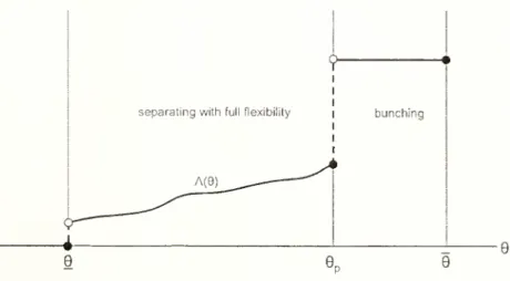
separatingwithfullflexibility

Figure 2:

The

Lagrange

multiplier

A

_{0)

Proposition4 showsthat under assumption

A

the optimal allocation is extremely

simple. It can be

implemented

by imposing a

maximum

level ofcurrent consumption,

or equivalently, a

minimum

level of savings.

Such

minimum

saving policies are a pervasive part of social security systems around the vi^orld.

The

next result

shows

the comparative statics ofthe optimal allocation with re-spect to temptation/5.

As

the temptation increases, i.e. /? decreases,

more

types are

bunched

(i.e. 6p decreases). In terms of policies, as the disagreement increases the

minimum

savings requirement decreases so there is less flexibility in the allocation.

Proposition

5 The bunching point 9p increases with j3.

The

minimum

savings

re-quirement, Smin

=

y

—

C

{u{9p)) , decreases with j3.

Proof.

That

Op is weakly increasing follows directly

from

its definition.

To

see that

Smin is decreasing note that Smin solves

9pU' {y

-

Sm\n)

_{_}

..

and

that 9p,

when

interior, solves,

^-^

=

E[9\9>9p].

Combining

these,

we

obtain

E

[9\9

>

9p] U'[y

-

s^in)

/W

{smm)

=

1- Since

E[9\9>9p]

is increasing in 6p the result follows from concavity of

U

and

W.

3.4

Drilling

In this subsection

we

study cases

where

assumption

A

does not hold

and

show

that the allocation described in Proposition 4 can be

improved

upon

by

drilling holes in

the separating section

where

the condition in assumption

A

is not satisfied.

Suppose

we

are offering the unconstrained

optimum

for a closed interval [9a,Oi,] of

agents

and we

consider

removing

the

open

interval _{{9a, Oh).} Agents that previously found their tangency within the interval will

move

to one ofthe two extremes, 9a or

6b.

The

critical issue inevaluating the changein welfare iscounting

how

many

agents

moving

to 9a versus Oi,. For a small

enough

interval, welfare rises from those

moving

to 9a

and

falls from those

moving

to 9h.

Since therelative

measure

ofagents

moving

tothe right versus theleft depends

on

the slope of the density function this explains its role in assumption A. For example,

if /'

>

then

upon

removing _{{0a, Oh)}

more

agents

would

move

to the right than the

left.

As

a consequence, such a change is undesirable.

The

proof of the next result

formalizes these ideas.

Proposition

6 Suppose an allocation {u,w) has {u{9)

,w

{9))

=

(u* {6),w* {9)) for

6

€

[^a,^fc] with db

<

9p. If the condition in assumption

A

does not hold /o7' 9 G

[9a,9),] then removing the interior of the set {{u* {9) ,

w*

_[9]) for9

G

_(&„,9b)} improves

welfare.

Proof. In the appendix.

Propositions 6 illustrates by construction

why

assumption

A

is necessary for a simple 'thresholdrule' to be optimal

and

gives

some

insight into this assumption.

Of

course. Proposition 6only identifies particular

improvements whenever

assumption

A

fails.

We

have not characterized the full

optimum

when

assumption

A

does not hold.

It seems likely that

'money

burning'

may

be optimal in

some

cases.

4

Arbitrary

Finite

Horizons

We

now

show

thatourresultsextend toarbitraryfinitehorizons.

We

confine ourselves to finite horizons because with infinite horizons any

mechanism

may

yield multiple

equilibria in the resulting game.

These

equilibria

may

involve reputation in the sense that a

good

equilibrium is sustained by a threat of reverting to a

bad

equilibria

upon

a deviation.

Some

authors have questioned the credibility of such reputational

equilibria inintrapersonal

games

(e.g.

Gul and

Pesendorfer, 2002a,

and

Kocherlakota,

1996).

We

avoid these issues by focusing

on

finite horizons.

Considerthe

problem

with

N

<

oo periods t

=

1, ...,TV

where

thefelicity function

is

U

(•) in each period. Let 9^

=

(6'i,^2, •,^t) denote the history ofshocks

up

to time

t.

A

direct

mechanism

now

requires that at time t the agent

make

reports

on

the

history of shocks r*

=

{r\,r2,

_,rl).

The

agent's

consumption

is allowed to

depend

on the whole history of reports:

_q

{r^,r^~^, ...,r^).

A

strategy for self-t is a

mapping

from the history of shocks

and

past reports into current reports: /?* (6'*,r'~\

••,'"^)-Truth

telling requires R^ {9^9*-'^,...,9^)

=

9^ _for all t

and

all histories 9K

We

first argue that without loss in optimahty

we

can restrict ourselves to

mecha-nisms that at time t require only a report r^ on the current shock _9t,

and

not of the whole history ofshocks 6*. This is the case in Atkeson

and

Lucas (1995) but in their

setup since preferences are time-consistent there is a single player

and

the

argument

is straightforward.

In contrast, in the hyperbolic

model

we

have A'' players

and

the difference in

preferences

between

these selves can be exploited to punish past deviations. For example, an agent at time t that is indifferent between allocations can be asked

to choose

amongst

them

according to whether there has been a deviation in the

past. In particular, she can 'punish' previous deviating agents by selecting the worst

allocations

from

their point ofview. Otherwise, ifthere have been no past deviations,

shecan 'reward' thetruth-telling agents

by

selecting theallocation preferred

by

them.

Such

schemes

may

make

deviations

more

costly, relaxing the incentive constraints,

and

are thus generally desirable.

One way

to

remove

the possibility of these

punishment

schemes is to introduce the refinement that

when

agents are indifferent between several allocations choose the one that

maximizes

the utility ofprevious selves. Indeed,

Gul

and

Pesendorfer's (2001,2002a,b) framework, discussed in Section 6, dehvers, in the limit without

self-control, the hyperbolic

model

with this

added

refinement.

However, with a continuous distribution for 9 such a refinement is not necessary

to rule out these

punishment

schemes.

We

show

that for any

mechanism

the subset

of over

which

^-agents are indifferent is at

most

countable. This implies that the probability that future selveswillfind themselves indifferent is zero so thatthe threat

of using indifference to punish past deviations has no deterrent effect.

For any set

A

of pairs (^i,

w)

define the optimal correspondence over x

E

X

M

[x;

A)

=

arg

max

{xu

+

w}

{u,w)eA

(we allow the possibility that

M

{x,

A)

is

empty)

then

we

have the following result.

Lemma

(Indifference is countable).

For

any

A

the subset

X^ C

X

for which

M

(x;

A)

has two or

more

points (set of agents that are indifferent) is at

most

count-able.

Proof.

The

correspondence

M

{x;A) is

monotone

in the sense that if xi

<

X2

and

21

(ui.wi) e

M{xi;A)

and

(u2,u'2)

€

M{x2;A)

then ui

<

U2- Thus, in an obvious

sense, points at which there are

more

than a single element in

M

{x;

A)

represent

upward

'jumps'.

As

with

monotonic

functions, it follows easily that

M

(.t;

A)

can

have at

most

a countable

number

ofsuch 'jumps'.

This result relies only on the single crossing property of preferences

and

not

on

the

linearity in

u and

w.

We

make

use ofthis

lemma

again in Section 5.

These

considerations lead us to write the

problem

with A'^

>

3 remaining periods

recursively as follows.

N

Period

Problem

vn

(y)

=

max

_/

[OU (c (9))

+

v^-i {y [9))] clF{9)

c,y

J

9U

{c{9))

+

(3vr,-i [y' _[9])

>

9hU

(c

(9)^

+

3v^^,

(ij (/5)) for all 9,9

^Q

c _{9)

+

y' {9)

<

y for all ^ G

9

where 112 (•)

was

defined in Section 2.

In the above formulation

we

assume, without loss in optimality, that the optimal

mechanism

is ex-post optimal given the resources available i.e. t',v-i

shows

up

in the

objectivefunction

and

incentive constraint. Thisis without loss in optimality because any inefficient continuation utility w' {9)

<

v^-i [y'_[9)) can be achieved

by

'money

burning' with the

same

effect: setting xu' {9)

=

i'at-i (y'[9)) for

some

y' [6)

<

y' {9).

For the simple recursive representation to obtain it is critical that, although the

principal

and

the agent disagree

on

the

amount

of discounting between the current and next period, they both agree

on

the utility obtained from the next period on,

given by uw-i- This is not true in the alternative setup where the principal

and

the agent both discount exponentially but with different discount factors.

We

treat this case separately in Section 7.

For

any

horizon A'' this

problem

has exactly the

same

structure as the two-period problem analyzed previously, with the exception that Vjsi-i (•) has substituted

W

{).

We

only required

W

{) to be increasing

and

concave

and

since I'yv-i (•) has these

properties allthe previous resultsapply.

We

summarize

this result in the next

propo-sition.

Proposition

7

Under

assumption

A

the optimal allocation vnth a horizon of

N

pe-riods can be implemented by imposing a

minimum

amount

ofsaving St {yt) inperiod

t.

In Proposition 7 the

minimum

saving is a function of resources yt-

With

CRRA

preferencesthe optimal allocationis linearly

homogenous

in_y, sothat c_{9,y)

=

c_{9)y

and

y'_{9,y)

=

_{y' {9) y.} It follows that the optimal

mechanism

imposes a

minimum

saving rate for each period that is independent of

yt-Proposition

8

Under

assumption

A

and

U

(c)

=

c^^'^/ {I

—

a) the optimul

m.echa-nism

for the N-period problem imposes a

minim.um

saving rate St for each, period t

independent

ofyt-4.1

Hidden

Savings

Another

property ofthe optimalallocation identified in Propositions 4

and

7is worth

mentioning.

Suppose

agents can save, but not borrow, privately behind the planner's back at the

same

rate ofreturn as the planner, as in Cole

and

Kocherlakota (2001).

The

possibility ofthis 'hiddensaving' reduces theset ofallocations that are incentive

compatible sincetheagent has astrictlylargerset ofpossible deviations. Importantly, the

mechanism

describedin Proposition 7 continuesto

implement

the

same

allocation

when we

allow agents to save privately,

and

thus remains optimal.

To

prove this claim

we

argue that confronted with the

mechanism

in Proposition

7 agents that currently have

no

private savings

would

never find it optimal to

ac-cumulate private savings.

To

see this, first note that by Proposition 7 the optimal

mechanism

imposes only a

minimum

on savingsin each period.

Thus

agent-^ always have the option ofsaving

more

observablywiththeprincipal than

what

the allocation

recommends,

yet by incentive compatibility the agent chooses not to.

Next, note that saving privately

on

his

own

can be

no

better for the agent than increasing the

amount

ofobservable savings with the principal. This is true because the principal maximizes the agents utility given the resources at its disposal. Thus, fromthe point ofviewofthecurrentself, futurewealthaccumulated by hiddensavings

is

dominated by

wealth accumulated with the principal.

It follows that agents never find it optimal to save privately

and

the

mechanism

implements the

same

allocation

when

agents can or cannot save privately.

Proposition

9

Under

assumption

A

the m.echanism described

m

Proposition 7

im-plern.ents the sam.e allocation

when

agents can save privately.

5

Heterogeneous

Temptation

Consider

now

the case where the leveloftemptation,

measured

by,i5, israndom. Het-erogeneity in_f3 captures the

commonly

held viewthat thetemptation tooverconsume

is not uniform in the population

and

that it is the agents that save the least that

are

more

likely to be 'undersaving' because of a higher temptation to

consume

(e.g.

Diamond,

1977).

Ifthe heterogeneity in temptation were due to

permanent

differences across

indi-viduals then the previous analysis

would

apply essentially unaltered. If agents

knew

their /3 at time time they

would

truthfully report it so that their

mechanism

could be tailored to their /3 as described above"*.

To

explore other possibilities

we assume

the other extreme, that differences in temptation are purely idiosyncratic, so that j3

is i.i.d. across time

and

individuals. Thus, each period 9

and

(3 are realized together

from a continuous distribution -

we

do

not require independence of 6

and

[3 for our

results.

We

continue to

assume

that /3

<

1 for simplicity.

For any set

A

of available pairs [u,

w)

agents with {6,/3)

maximize

their utility:

/^

arg

max

<

—u +

w

{u,w)eA _yjj

Note

thatthis arg

max

set is identical for alltypes withthe

same

ratio

x

=

_9/

^

which implies that

we

can without loss in optimality

assume

the allocation

depend

only on

X.

To

see this note that the allocation

may

depend

on 9

and

/3 independently for

a given x only if the x-agent is indifferent

amongst

several pairs of u,w. However, the

lemma

in section 4

showed

that the set of x for which agents are indifferent is

*0fcourse, ifagents canonly report at f

=

1 then one cannot costlesslyobtain truthful! reports on(5. However, with largeenough

N

it is likely that the cost ofrevealing /3 would besmall.

of

measure

zero.

As

a consequence, allowing the allocation to

depend

on 6 or /3

independently, in addition to x, cannot improve the objective function.

Without

loss in optimality

we

limit ourselves to allocations that are functions ofx only^.

The

objective function is then:

E

[eu(x)

+

w

{x)]

=E[E

[Ou (x)

+

w

(x)| x]]

=

f

[a (x)

u{x)

+ w

(x)]

_/

(x)

dx

where

a

(x)

=

E

{6\x)

and

_/ (x) is the density over x. Let

X

=

[x,x] be the support

ofX

and

F

(x) be its cumulative distribution.

Define Xp as the lowest value such that for x

>

Xp

E

[a(x)|X

>

x]

X

"

We

modify our previous assumption

A

in the following way.

Assumption

A.

For x

e

[x,Xp],

we

have that

xf'ix)^

2-«'(x)

/(x)

-

l-a(x)/x

Note

that without heterogeneity

a

(x)

=

/3x so that assumptions

A

and

A

are

equivalent in this case.

Heterogenous

Temptation

Problem

max

/

{a

(x)u[x)

+

w

(x)}

dF

(x)

<-)M)

J

subject to

xu

(x)

+

ly(x)

=

xu

(x)

+ w

(x)

+

u

(x)

dx

c{u{x))

+

k{w{x))

<

1

u{x)

>

u

_(y) for all

x

>

_y

^Given/3

<

1 a simplerargumentisavailable. Theplanner can simplyinstructagentswithgiven X to choose the elementofthe arg

max

with the lowest u, since the planner has a strict preference

for the lowestuelement. The argument inthe textissimilar to the one usedto extendthe analysis to arbitraryhorizonsand can be appliedto the case where/?

>

1 is allowed.

The

proofofthe next result closely follows the proofof proposition 4.

Proposition 10

Under

assumption

A

agents with x

<

Xp are offered their

uncon-strained

optimum and

agents with x

>

Xp are bunched at the unconstrained

optimum

for agent Xp.

6

Commitment

with

Self

Control

Gul

and Pesendorfer (2001,2002a,b) introduced an axiomatic foundation for

prefer-ences for

commitment.

We

review their setup

and

representation result briefly in

general terms

and

then describe

how

we

apply it to our framework.

In their static formulation the primitive is a preferences ordering over sets of choices, with utility function

P

{A) over choice sets A. In the classical case

P

(A)

=

maXagyip(a) for

some

utility function p defined directly over actions.

Note

that in this case if a set

A

is reduced to A' without removing the best element, a* from A, then

P

is not altered. In this sense,

committment,

a preference for smaller sets, is

not valued.

To

model

a preference for

commitment

they

assume

a

consumer

may

strictlyprefer

a set A' that is a strict subset .4, i.e.

P

{A')

>

P

(.4)

and

A'

C

A.

They

show

that such preferences can be represented by two utility functions

U

and

V

over choices a by the relation:

P

{A)

=

max

_{p(a)

+

t{a)}

— max

t(a)

a€.4 ae.4

One

can think of t(a)

—

maXag^

t(o) as the cost of self-control suffered

by

an agent

when

choosing a instead of

argmax^g^i

(a). In a

dynamic

setting recursive

prefer-ences with temptation can be represented similarly (Gul

and

Pessendorfer (2002a,b). In our

framework

the action is a choice for current

consumption and

savings, c

and

k. In order to nest the hyperbolic preferences

model

we

follow Krusell,

Kuruscu

and Smith

(2001)

and

use:

p

(c,k)

=

On(c)

+

w

{k)

t (c,k)

=

(p[On(c)

+

i5w(A:))

where

the parameter

>

captures the lack ofself control.

As

—

^ oo the agent has noself-control

and

yields fully to his temptation. His preferences essentially converge

to those implied

by

the

hyperboHc

model.

The

only difference is that in the limit as

—

* oo

we

obtain a tie-breaking criteria that

whenever

an agent is indifferent he

selects whatever is best for his previous 'selves' (i.e. maximizes t).

The

objective function is:

/ {9u{e)

+

w{e))f{9)de

+

(p {9u{9)

+

pwie))f{9)de

Je Je,

-(p f

[9u{9)+l3w{9))f{9)d9

Je,

where

{u,

w)

is the allocation for the "temptation agent"

and

{u,

w)

is the allocation ofthat is chosen

by

the "self-control agent". It is convenient to define everything for

asupport larger than

9

given by

=

[9, 9]

where

9

=

9/3/13

<

9.

Given asetof offered (m,

w)

pairs,the "self-control agent" will choose anallocation

that

maximizes 9u

+

f3w with /3

=

(1

+

4>/3)/(1

+

0), while the "temptation agent" will choose

an

allocation that maximizes

9u

+

(3w. Since both the "temptation"

and

the "self-control" agents choose from the

same

set it follows that,

u{9)=u{9l3/P),

(8)

so that the "self-control agent" 9 acts as a "temptation-agent" with a lower taste

shock.

Substituting (8) into the objective function

we

obtain,

(1

+

0) /" (9u (^/3//3)

+

/3io (913/l3\) f {9) d9

-

4>

f

{9u{9)

+

(3w{9))

f

(9) d9.

The

first

term

can be

shown

to equal,

(1

+

(/.)13//3

/ {9u{9)

+

f3iu {9))

f

(9P/I3) P/pd9. JiJ3/0 ^ '

Note that h[9)

=

_f (9p//3] ^/l3 is thedensity ofthe

random

variable_9P/^; let

H

_{9) represent its corresponding distribution function.

The

objective function can be written as,

3 rS-e r§

(1

+

<^)

§

r

{9u(9)

+

/3w(9))

hi9)d9-d

{9u(9)

+

Biv{9))

f

(9) d9.

Substituting in the incentive constraint,

9u

(9)

+

/3w{9)

=

I u{9)de

+

vo,

Je

where vq

=

{9J3/P)u{9)

+

(3w{§)

and

integrating

by

parts,

we

obtain:

{l

+

(P)^Jf

il-H{9))u{9)de-(l>J^

{l-F{9))uie)d9+(^il

+

<P)p/l3-cP^vo.

where

we

are taking both intervals of integration as being from ^ to ^

by

letting

h{9)

=

0, for all 9

>

^/3//5

and /

(^)

=

for all 9

<

9. In addition

we

require

u

to be non-decreasing

and

the budget constraint:

vo+

(

u _{(9^ d9}

-

9u

{9)

<

(3K~' {y

-

C

{u{9)))

.

Definition. Let 9p be the lowest value such that for 9

>

_9p,

y_7(l

+

0)

_^

(1

-

^

m

-<P{1-F

{9))] d9

<

Assumption

A.

For 9

€

[9,9p],

we

have that

(l

+

_{,/.)(/3//3)'/(^/3//3)-0/W>O}

We

now

show

that the optimalallocation is to offer all types below 9p their

uncon-strained

optimum

and

to

bunch

types higher than 9p at the unconstrained

optimum

for 9p.

Denote

this allocation by {w*,u) as before.

The

Lagrangian is

L

=

_jU{l

+

<l>)^{l-H{9))-<l>{l-F{9))-il-A{e))\u{e)d9

+

_/ {/3K-'

{y-C

{u₍₉₎₎₎₊9ii)

dk

/3

+

l(l+</>)^-0

(l-A(0)No

where

A

isa non-decreasing Lagrange multipUer for thebudget constraint,

normahzed

so that A(^)

=

1.

Proposition

11

The

allocation {w*,u) is optimal ifand only ifassumption

A

holds.

Proof.

We

follow the proofof Proposition 4 as closely as possible.

At

the proposed

allocation

we

have:

dLiw,u-h^Ji^\A)=

_l^{{l

+

<P)^{l-H{9))-cl){l-F{9))-{l-A{9))]h^{9)d9

+

(^P

l^^[^f^-^]\\9..e]hudA

+

;i

+

0)|-(/.-(l-A(^))

L,

Equation (5) requires

A{9)

—

{1

+

4>) (/3//9

—

1). Using this

and

integrating (3)

by

parts leads to

dL

{w,u-/i„, /),„!A)

=

7

[9) hu

{9)+

7 (0)dh^, {9) (9)

where,

^{9)^

Nil

+

4>)t

_[I-

H

_{{9))- <t^{l-F [9))-}

_{I-

_{K{9))\d9+e,j'^(^~^}

It follows that (4) requires

7

(^i)

=

for 9

G

9,9r, , i.e.

where

u is strictly increasing.