Conflicts of Interest and Steering in Residential Brokerage
The MIT Faculty has made this article openly available.
Please share
how this access benefits you. Your story matters.
Citation
Barwick, Panle Jia, Parag A. Pathak, and Maisy Wong. “Conflicts of
Interest and Steering in Residential Brokerage.” American Economic
Journal: Applied Economics 9, no. 3 (July 2017): 191–222. © 2017
American Economic Association
As Published
http://dx.doi.org/10.1257/APP.20160214
Publisher
American Economic Association
Version
Final published version
Citable link
http://hdl.handle.net/1721.1/114048
Terms of Use
Article is made available in accordance with the publisher's
policy and may be subject to US copyright law. Please refer to the
publisher's site for terms of use.
191
Conflicts of Interest and Steering in Residential Brokerage
†By Panle Jia Barwick, Parag A. Pathak, and Maisy Wong*
This paper documents uniformity in real estate commission rates offered to buyers’ agents using 653,475 residential listings in
east-ern Massachusetts from 1998–2011. Properties listed with lower commission rates experience less favorable transaction outcomes: they are 5 percent less likely to sell and take 12 percent longer to sell. These adverse outcomes reflect decreased willingness of buyers’ agents to intermediate low commission properties (steering), rather than heterogeneous seller preferences or reduced effort of listing agents. Offices with large market shares purchase a disproportion-ately small fraction of low commission properties. The negative out-comes for low commissions provide empirical support for regulatory concerns over steering. (JEL D82, L85, R21, R31)
B
uyers are routinely advised by salespeople or intermediaries who are compen-sated by sellers. In many settings, there are concerns that buyers are steered towards products that are not in their interest.1 We study this phenomenon for resi-dential real estate, where intermediaries play an important role. In 2014, there were 4.94 million existing home sales valued in aggregate at $1.26 trillion dollars, and real estate agents assisted in 88 percent of sales (NAR 2014a, 2015).2 Brokerage commissions constitute a major component of housing transactions costs.Regulators have repeatedly expressed concerns that high and uniform commis-sion rates in the residential brokerage industry point to collusive behavior. The cen-tral question is how this structure can be sustained despite low entry barriers and a seemingly competitive marketplace with many firms and agents. One often cited factor is steering. In the conventional compensation arrangement where sellers pay
1 See Cummins and Doherty (2006) for a discussion on insurance products; Inderst and Ottaviani (2012) for
financial advice; Jiang, Stanford, and Xie (2012) for bond ratings; Christoffersen, Evans, and Musto (2013) for mutual funds; Chan, Haughwout, and Tracy (2015) for mortgages; and Shapiro (2015) for the health sector.
2 Throughout this paper, an “agent” is an individual who assists buyers or sellers in housing transactions, an
“office” or a “firm” is a broker that an agent works for, and an “agency” refers to an agent and her broker. * Barwick: Department of Economics, Cornell University, 462 Uris Hall, Ithaca, NY 14853 and NBER (email: panle.barwick@cornell.edu); Pathak: MIT, 50 Memorial Drive, Cambridge, MA 02142 and NBER (email: ppathak@mit.edu); Wong: Wharton Real Estate, 3620 Locust Walk, Philadelphia, PA 19104 (email: maisy@ wharton.upenn.edu). We thank Steven Berry and Peter Reiss for suggestions in the early stage of this project. We also thank Matthew Backus, Joe Gyourko, Robert Masson, Debi Prasad Mohapatra, Wenlan Qian, Todd Sinai, Nancy Wallace, participants at Cornell, the Department of Justice, NBER Summer Institute, WFA Real Estate Symposium, University of Washington, Wharton, and Yale for helpful comments. We thank the referees for their comments. We are grateful for the excellent research assistance of Ying Chen, Xuequan Peng, and Jeremy Kirk, and to Paul Amos for assistance with GIS. Barwick acknowledges the research support from the National Science Foundation via grant SES-1061970. Wong acknowledges financial support from the Research Sponsors Program of the Zell/Lurie Real Estate Center at Wharton.
† Go to https://doi.org/10.1257/app.20160214 to visit the article page for additional materials and author
for the commissions of their listing agents and potential buyers’ agents, the latter have an incentive to prioritize properties that offer higher commissions. According to a 1983 report by the Federal Trade Commission (F TC), “(s)teering … may make price competition a potentially unsuccessful competitive strategy, and it is our belief that this is the most important factor explaining the general uniformity of commis-sion rates” (Los Angeles Regional Office 1983, 12). To date, the current commis-sion structure remains an important subject of policy debate and regulatory concern (GAO 2005, F TC and USDOJ 2007).
We investigate the consequences of steering behavior on sales outcomes using a dataset that includes commission rates offered to buyers’ agents for 653,475 listed properties in eastern Massachusetts from 1998 to 2011. In addition, we observe detailed information on property attributes, agents, and brokerage offices that are involved in each transaction. Ninety percent of properties in our sample have a buy-ing commission of 2.0 or 2.5 percent,3 corroborating the common perception that commission rates are uniform. In addition, even in periods with substantial turnover among real estate brokerage firms and agents, the average commission rate exhibits only modest fluctuation.
After documenting limited commission variation in our sample, we track the per-formance of offices with different commission rates. We find that offices charging lower commission rates are much less likely to become the top 25 percent firms in terms of commission revenue or the number of listings, relative to comparable offices that charge higher commissions. Standard competitive forces, whereby a firm competes with rivals using lower prices, do not seem effective under the current commission arrangement.
This finding motivates our core analysis that examines the sales outcomes of properties listed with different buying commission rates. Consistent with real estate agents steering buyers to properties with high commissions, we find that if a prop-erty has a buying commission rate less than 2.5 percent, it is 5 percent less likely to be sold and takes 12 percent longer to sell, compared to properties that offer buying agents 2.5 percent or more. There is little effect on the sale price. While it is possible that lower commission rates are associated with less desirable property attributes, our estimates are robust to specifications that include a rich set of property level measures that control for time-varying attributes and property fixed effects that con-trol for time-invariant attributes.
We address two additional threats to our empirical analysis. First, the poor per-formance of low commission properties may reflect reduced listing agent effort, rather than an unwillingness of buyers’ agents to be involved in low commission properties. To investigate this possibility, we report specifications focusing on prop-erties that are more homogenous and relatively easier to sell. Then we control for time-invariant agent attributes using listing agent fixed effects. Third, we construct “pairs” of properties that are listed by the same agent in the same year with listing commission revenues within a $500 bin, but offer different commission rates to the buying agent. Since these properties have the same payoff for the listing agent,
3 These correspond to a total commission of 4 percent or 5 percent, respectively, if commissions are equally split
they should induce the same level of effort from the listing agent, but may attract a different number of buyers given the difference in buying commission rates. In this demanding analysis that exploits variation within an agent, property type, year, and commission bin, we continue to find that listings offering lower commission rates are associated with lower sales probabilities. All three investigations suggest that unobserved listing agent effort is not driving our main results.
The second threat we examine is that the adverse sales outcomes do not simply reflect behavior of buying agents, but the preferences of sellers. Some sellers might be more patient and willing to trade off a low sale probability with a high sale price. If these sellers are more likely to work with firms charging low commissions, then our results would be confounded by seller heterogeneity. We tackle this issue in several steps. First, we control for seller urgency using list price as a proxy. Next, we construct a patience index, which is the ratio of the observed listing price to the predicted price from a hedonic regression. More patient sellers have higher index values. Sellers are divided into 10 or 100 groups according to this index. We use these group dummies as controls for seller patience. Finally, we merge our data with property deeds that record seller and buyer names and estimate models using seller fixed effects. Our analysis continues to report negative sales outcomes associated with lower commis-sion rates, even accounting for fixed and time-varying seller preference.
After ruling out these alternative explanations, we show that properties that are more susceptible to steering suffer worse outcomes. For example, the sale proba-bility and days on market worsen monotonically when we compare three groups of listings that offer more than 2.5 percent, exactly 2.5 percent, and below 2.5 percent, respectively. This is consistent with the fact that properties offering higher commis-sion rates provide stronger financial incentives. Similarly, we find worse outcomes for low commission listings in neighborhoods with a larger fraction of high commis-sion listings, listings by entrants, and listings by offices that used lower commiscommis-sion rate policies in the past.
To understand why low commission listings have worse performances, we exam-ine the transaction patterns of dominant offices that intermediate a large fraction of purchases. We find that firms with higher market shares buy a smaller fraction of low commission properties. While our core analysis at the property level demonstrates that all firms prefer properties with high commissions, these results illustrate lower propensity of dominant firms to intermediate low commission properties. If we assume that dominant firms’ diminished willingness to purchase low commission properties leads to a reduced number of potential buyers, this finding can explain about 40 percent of the adverse sales outcomes reported above.
This paper makes several contributions. First, we construct a large dataset that documents individual buying commissions for about half a million properties and spans an entire housing business cycle. Second, to our best knowledge, we provide the first causal analysis of the consequence of buying agent commissions on eco-nomic outcomes. We use data from the traditional brokerage platform (the Multiple Listing Service) that accounts for the majority of real estate transactions and pres-ent evidence that supports regulators’ concerns over steering behavior. Third, our paper highlights distortions when incentive schemes serve a dual role of eliciting agent effort and matching buyers and sellers. The negative consequences of low
commissions reported here arise from the fact that sellers have only one instrument for two distinct purposes: to incentivize effort and to attract buyers’ agents.
Our paper contributes to several literatures. The first literature studies implica-tions of the fixed percentage commissions in the real estate brokerage industry (such as, Hsieh and Moretti 2003, Levitt and Syverson 2008b, and Han and Hong 2011. See Han and Strange 2015 for a review).4 Our paper is most similar to Levitt and Syverson (2008a) that studies listings by flat fee or limited service agencies and Hendel, Nevo, and Ortalo-Magné (2009) that focuses on For-Sale-by-Owner (FSBO) transactions. Our results on steering behavior also resonate with other work docu-menting that consumers often receive advice from experts that is not in their inter-est. For example, Mullainathan, Noeth, and Schoar (2012); Christoffersen, Evans, and Musto (2013); and Del Guercio and Reuter (2014) study financial advisers and broker recommendations for mutual funds; Jiang, Stanford, and Xie (2012) ana-lyze bond ratings; Schneider (2012); Anagol, Cole, and Sarkar (2017); and Shapiro (2015) examine the auto repair, insurance, and health industries, respectively.
Another related literature examines whether incentive schemes have adverse consequences on agent performance. Oyer (1998) investigates the implications of nonlinear incentive schemes on fiscal targets. Larkin (2014) uses data from an enter-prise software vendor to demonstrate the gaming of the deal closure time by sales-people in response to the vendor’s accelerating commission schedule.
The rest of this paper is organized as follows. Section I discusses the institutional background. Section II describes the data and presents descriptive patterns of the housing market and commissions during our sample period. Section III analyzes property level sales outcomes for low commission properties. Section IV explores why low commission properties suffer worse outcomes. In Section V, we discuss the costs of a low commission rate strategy for home sellers. Section VI concludes. Online Appendix A explains market definition and how we construct regressors used in our analysis. Additional results are presented in online Appendix B and C, with Figure B1 in online Appendix B and Tables C1 to C9 in online Appendix C.
I. Institutional Background
Real estate agents are licensed intermediaries who provide services to buyers and sellers in real estate transactions. The licensing requirements for Massachusetts are modest (see Barwick and Pathak 2015 for more details). For home sellers, agents help to advertise the house, suggest listing prices, conduct open houses, and negoti-ate with buyers. For home buyers, agents search for houses that match their clients’ preferences, arrange visits to the listings, and negotiate with sellers. Agents can influence buyers’ decisions in several ways, including which properties to show, which property attributes to highlight, and how much effort to exert during the offer and negotiation stages. Therefore, steering, which is known as “sell to the commis-sion” in the industry (Harney 2015), can manifest along multiple dimensions.
4 Other recent work on real estate agents includes Rutherford, Springer, and Yavas (2005); Nadel (2007); Jia and
A contract between the seller and the listing agency usually includes the list price and the total commission the seller is obligated to pay to the listing agency in the event of a sale. Commissions are often quoted as a certain percentage of the sale price. In the greater Boston area, the norm for this rate is 5 percent. The National Association of Real Estate Exchanges (the predecessor to the National Association of Realtors (NAR)) institutionalized a commission rate norm when it adopted its first Code of Ethics in 1913. It stated that “(a)n agent should always exact the reg-ular real estate commission prescribed by the board or exchange of which he is a member.” In Boston, agents referred to the schedule of Broker’s commissions published regularly by The Boston Real Estate Exchange (BREE). In the 1920s, the typical commission rate for the city of Boston was 2.5 percent (Benson and North 1922).5 This rate increased to 5 percent in 1940 and has prevailed ever since as the most common rate for listings in the area (BREE 1940).
This paper focuses on the common practice of bundling commissions, where a seller pays one commission to her listing agency, who then shares the total commis-sion with the agency who finds a buyer. In particular, the commiscommis-sion rate paid to the buying agency is specified in the listing agreement prior to the knowledge of buying agents. When buying agents are informed of properties, they observe the property attributes as well as the buying commission rate for each property (buyers do not observe the commission rate). This practice began in the early twentieth century to minimize the problem of buyers and sellers circumventing the payment of brokerage fees (Davies 1958, Wachter 1987).
In many cases, the commission fee is evenly split between the listing and buying agencies. The 1913 Code of Ethics, for example, specifies that the eighth duty of members is to “… always be ready and willing to divide the regular commission
equally with any member of the Association who can produce a buyer for any cli-ent.” 6 More recent data suggest this pattern of equal splits persists until today. To investigate the commission split between listing and buying agencies, we collect a random sample of 70 HUD-I housing settlement statements from 39 brokerage offices in 37 of our sample markets. A HUD-I settlement statement itemizes all financial obligations of the borrower and seller in a real estate transaction, includ-ing commissions paid to and rebates from the buyinclud-ing and sellinclud-ing agencies. About 90 percent of transactions in this random sample have even splits of commissions. For the remaining transactions, half pays more to the listing agency, and half pays more to the buying agency.
The commission to an agency is further split between agents and their brokers. According to a 2007 survey conducted by the NAR, most agents are compensated under a revenue sharing arrangement, with the median agent keeping 60 percent of her commissions and submitting 40 percent to her firm (Bishop, Barlett, and Lautz 2007). Similar to salespeople working in other professions (Joseph and Kalwani 1998), many brokerage firms also include built-in “accelerators” that entail pro-portionately higher earnings with higher gross commission revenue. For example,
5 The fee was 2.5 percent up to $40,000 (or $460,000 in 2011 dollars) and 1 percent on the balance, with a
minimum of $100.
a major franchise, Keller Williams, has a profit sharing arrangement with “an elab-orate seven-step function” that shares more with more productive agents (Inman 2014). Such nonlinear incentive schemes that are based on revenue further enhance agents’ preferences toward listings with higher commission rates.
To illustrate how commissions are typically split between agents and brokers, suppose a property is worth $500,000 and the commission rate is 5 percent. The total commission is $25,000. The listing and buying agencies are compensated $12,500 each, which is further split so that the agent gets 60 percent ($7,500) and the broker receives 40 percent ($5,000).
II. Data and Descriptive Patterns
A. sample coverage
The data for this study come from the Multiple Listing Service (MLS) network for eastern Massachusetts, a centralized platform containing information on prop-erty listings and sales. This area has a number of virtues for our analysis: the market experienced a boom-bust cycle during our sample period, with house prices peaking in mid-2000s and falling thereafter. The market also includes high priced subur-ban towns with single-family homes and more densely populated inner ursubur-ban areas where condominiums make up the bulk of transactions.
We collect information on all listed non-rental residential properties. Our sample contains 653,475 listings between 1998 and 2011, covering 85 towns and cities surrounding Boston. We combine 12 small cities with their closest neighbor. Given the size of Boston, we split it into 15 markets using Zillow’s definition of neighbor-hoods and a variable in the MLS (area) that identifies neighborhoods within cities. This gives us a total of 87 markets. Online Appendix A provides more details on the sample construction and market definition.
For each listed property, we observe listing details (the listing date and price, the listing office and agent, the commission rate offered to the buyer’s agent, and so on), a rich set of property characteristics, and transaction details when a sale occurs (the sale price, date, the purchasing office, and agent). The number of days on the market is measured by the difference between the listing date and the date the property is removed from the MLS database. We complement the MLS data with a deeds data-set from a commercial vendor that records seller and buyer names for all properties that change ownership during 1998 to 2008. This allows us to track home buyers and sellers over time. We also merge in data from the Home Mortgage Disclosure Act (HMDA), which includes information on the income of buyers.
Our sample comprises three property types: condominiums (35 percent), single family homes (52 percent), and multifamily properties (13 percent). The average listing in our sample has 1,840 square feet, 3 bedrooms, 2 bathrooms, and is 62 years old. The median list price is $420,000 and the median sale price is $398,000 (both in 2011 dollars). The properties in our sample are comparable in size, but are older and more expensive than the average home purchased in the United States between 2013 and 2014 (NAR 2014b), which has 1,870 square feet, 3 bedrooms, 2 bathrooms, and is 20 years old with a median sale price of $235,000.
B. commission Fees
There is surprisingly little information on commissions at the property level. The only exceptions that we are aware of include Woodward (2008) and Schnare and Kulick (2009) that are prepared for the Department of Housing and Urban Development and for the NAR, respectively. They investigate variation in buying commissions across real estate markets but do not examine the consequences of buying commissions on sales outcomes.7 We are not aware of any study on US mar-kets that has information on listing commissions.
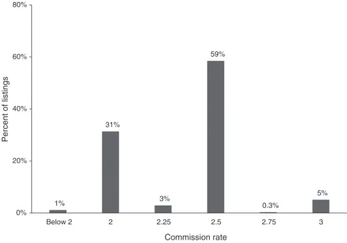
Critically, we observe the commission rate offered to buyers’ agents for each of our 653,475 listings. The histogram in Figure 1 establishes that the lion’s share of listings offer either a 2.5 percent or a 2 percent commission rate to the buyer’s agent, with the rest scattering between 2 and 3 percent. Specifically, the most commonly observed rates are 2.5 percent (59 percent of listings), 2 percent (31 percent of listings), 3 percent (5 percent of listings), and 2.25 percent (3 percent of listings). Throughout our analysis, we define a low commission rate listing as one with a buy-ing commission rate strictly below 2.5 percent and a high commission rate listbuy-ing as one with a rate at or above 2.5 percent. The only exception is Section IVA, where
7 Goolsby and Childs (1988) and Zietz and Newsome (2001) report on buying commissions for a few hundred
transactions. 1% 31% 3% 59% 0.3% 5% 0% 20% 40% 60% 80% Below 2 2 2.25 2.5 2.75 3 Percent of listings Commission rate Figure 1. Distribution of Commission Rates
notes: Distribution of commission rates offered to buyers’ agents. The figure reports data for 99.3 percent of list-ings. The rest are scattered between 2 and 5 percent.
we separate listings that pay exactly 2.5 percent from listings that pay more than 2.5 percent for some robustness analyses.
Commission rates display some geographical variation (Figure B1). Markets that are characterized by high household income and high house prices tend to have higher commissions. In addition, the average commission rate displays a modest U-shape over time, varying from 2.49 percent in 1998 to a low of 2.27 percent in 2005 before reverting back to 2.39 percent in 2011. This modest variation masks a relatively large change in the fraction of listings at 2.5 percent: about 74 percent in 1998, 49 percent in 2005 (a period with a large influx of entering agents and offices as documented in Barwick and Pathak 2015), and 62 percent in 2011.
Most offices have commission rate policies or norms. There appear to be sys-tematic differences in commission rates charged by different offices. Among the six dominant chains—Coldwell Banker, Century 21, Remax, Hammond, Prudential, and GMAC—only Century 21 has a majority of listings at rates below 2.5 percent. Coldwell Banker, the largest chain that accounts for about 20 percent of all listings in our sample, rarely lists properties at rates below 2.5 percent. In contrast, 48 per-cent of independent offices and smaller chains have a majority of listings at rates below 2.5 percent. The firm level commission variation could reflect differences in costs, such as overhead, insurance charges, technology, and marketing costs. It could also come from brand premium, prestige, and historical norms. Finally, there is evidence that firms set prices based on property types (condominiums usually list at high commission rates), demographics (such as average income of potential customers), and market conditions.
To investigate the sources of variation in commission rates, we present a set of regressions in Table 1 where the dependent variable is 1 if the commission rate for a listing is strictly below 2.5 percent ( rL25 ). Column 1 only controls for market con-ditions using market-year and month fixed effects. Column 2 only includes property controls and property fixed effects. Column 3 only controls for office fixed effects. Column 4 includes 178,000 office-year-market-property type fixed effects. In addi-tion to the r2, we also report how well we can predict rL25 . We first predict rL25 using the controls in each column. We then define ˆ rL25 as 1 if the predicted value is at least 0.5 and zero otherwise.8 The share of listings where ˆ rL25 equals rL25 is reported after the r2.
Across the columns, we are able to predict the low commission dummy with a high degree of accuracy, consistent with our discussion above that brokerage offices appear to be setting commission rates according to norms, market conditions, demo-graphics, and property types. The high r2 suggests that these are the primary determi-nants of commission rates. In particular, we can predict rL25 correctly for 91 percent of the listings using office-year-market-property type fixed effects (the r2 is 0.72). Moreover, recent statistics show that many sellers do not shop for agents. Seventy percent of home sellers contact only one agent before selecting the one to assist with their home sale (NAR 2014a). Only 3 percent of sellers report that the commission is the most important factor in choosing a listing agent (NAR 2013). The seemingly
8 We also experimented with defining ˆ rL25 as 1 when the predicted value is at least 0.3, 0.4, 0.6, and 0.7 instead
idiosyncratic manner in which sellers approach commission rates is consistent with the view that most sellers are inexperienced (Akerlof and Shiller 2015).
C. Brokerage Firms and Agents
There are a total of 8,888 offices and 35,129 agents in our dataset. The ability to observe agent and office identifiers as well as their past transactions allows us to construct detailed measures of office and agent quality, including experience, various sales performances (such as the fraction of listings that are sold each year, the average days on market), and property portfolio (the fraction of condominiums or single-family houses). For offices, we also observe the size and quality of their agents. We collect each office’s street address from a variety of data sources and use this information to construct distance between offices.
A large number of offices and agents have only a few listings throughout our sample period. Offices (agents) whose average annual listings are above five (two) are responsible for 95 percent (92 percent) of the listings.9
D. Growth Paths of Low commission Firms
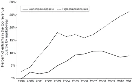
One interesting pattern is that entrants (brokerage firms established in 1999 or later) that offer low commissions are much less likely to reach the top tier of the market in terms of revenue than entrants with high commissions. In Figure 2, we classify entrants into a low commission rate group (solid line) and a high com-mission rate group (dashed line) based on their observed commission rates in the
9 The average annual number of listings is the ratio of the total number of listings by an office or agent over the
total number of years that office or agent spans our data (the last year minus the first year plus one). Table 1—Variation in Low Commission Listings
(1) (2) (3) (4)
r2 0.32 0.63 0.44 0.72
Fraction of correct predictions 0.78 0.87 0.81 0.91
Observations 653,475 344,832 653,475 653,475
Market-year, month fixed effects Yes No No No
Property controls, property fixed effects No Yes No No
Office fixed effects No No Yes No
Office-year-market-property type fixed effects No No No Yes notes: This table reports results from listing-level OLS regressions where the dependent vari-able is 1 if the commission rate is strictly below 2.5 percent. Column 1 controls for 1,228 market-year fixed effects and month fixed effects. Column 2 controls for 148 property con-trols and 133,902 property fixed effects. Column 3 concon-trols for 7,055 listing office fixed effects. Column 4 includes 178,291 office-year-market-property type fixed effects. The sample includes all listings, except for column 2, which has property fixed effects and is restricted to the sample of repeat listings only. To calculate the fraction of correct predictions, we first pre-dict the dependent variable after estimating the OLS regression in each column. We then define ˆ
rL25 to be 1 if the predicted value is at least 0.5 and 0 otherwise. Finally, we calculate the frac-tion of listings where ˆ rL25 is equal to the observed low commission dummy.
first three years. An entrant belongs to the low (high) commission rate group if its fraction of rL25 listings in the first three years is in the top (bottom) quartile among all entrants in the same market. We define “successful brokerage firms” as those whose listing revenues are ranked top quartile among all offices in the same market. Figure 2 illustrates the likelihood for low commission entrants and high commis-sion entrants to become successful over time. Both groups start small with a similar probability of being in the top quartile (less than 3 percent), but the gap widens over time. By the end of our sample period, entrants with high initial commission rates are 17 percent more likely to be in the top quartile than entrants whose initial commission rate is low. The pattern remains the same if we define the “top quartile” status using the number of listings instead of commission revenues.
One possible explanation is that entrants are not identical. Firms that are able to recruit talented agents or with more connections might charge a high commission rate and do well at the same time. When we adjust for observable differences between high and low commission firms in Table C1, we continue to find that firms with low commissions are less successful. These findings seem puzzling: competitive behav-ior, where offices charge low prices for comparable services, does not lead to suc-cessful outcomes. Instead of growing, these offices are more likely to remain small.
III. Results
Motivated by the patterns discussed above, our core analysis tests whether a low commission rate offered to the buyer’s agent affects the sale performance of a
Figure 2. Growth Paths for High and Low Commission Entrants
notes: Entrants are firms that first appear in our sample in 1999 or later. We classify entrants into the high commis-sion rate group and low commission rate group using their commission rates in the first three years. Entrant i is in the high commission rate group (or low commission rate group) if its fraction of high commission listings in the first three years is in the top 25 percent (bottom 25 percent) among all entrants in the same market. An entrant’s top-revenue-quartile status is defined using its listing commission revenue in a market and year against all offices in the same market-year.
0% 5% 10% 15% 20% 25% 30% 1999 2000 2001 2002 2003 2004 2005 2006 2007 2008 2009 2010 2011
Percent of entrants in the top revenue
quartile by market-year
listing. We first show that listings offering high versus low commission rates appear to be comparable, on average. We then present robust evidence that the effect of commission rates on sales outcomes survives a rich set of controls for market con-ditions, property characteristics, seller, agent, and office attributes, as well as an instrumental variable strategy.
A. Effect of commission rate on Transaction Outcomes Our main listing level regression is of the following form:
(1) y ipklmt = β 1 rL2 5 ipklmt + PrO P ipt β 2 + AG T kmt β 3 + OFFic E lmt β 4 + μ mt + τ month + π p + ε ipklmt ,
where y ipklmt is the sale outcome for the i th listing of property p , by agent k and office
l , in market m and year t .
The key regressor is rL25 , a dummy that is 1 if a listing offers a commission rate that is strictly below 2.5 percent. One major empirical challenge is that listings offering low commission rates may have less desirable attributes that lead to adverse outcomes ( β 1 may be downward biased). There are many sources of confounders in our context because houses are differentiated along multiple dimensions and many parties are involved in a housing transaction. We include controls for property char-acteristics ( PrOP ), attributes of listing agents ( AGT ) and listing offices ( OFFicE ), market-by-year fixed effects ( μ mt ) for time-varying market conditions, month fixed effects ( τ month ), and property fixed effects ( π p ). To conserve space, we reserve a detailed description of all controls in online Appendix A. We examine three perfor-mance measures of a listing: the sale probability, as well as the days on market and the sale price if a listing is sold.
The parameter of interest is β 1 . In an ideal setting where buying agents fully inter-nalize interests of their clients, how much agents are compensated should not affect the sale outcome ( β 1 should be zero, since buyers do not observe commissions). On the other hand, if buying agents steer their buyers toward high commission properties, a negative β 1 would reflect this conflict of interest. Our identification assumption is that rL25 is uncorrelated with the residual of sales outcomes, ε ipklmt , conditioning on our regressors. Section IIB presents evidence that firms set com-mission rates based on property types, demographics, and market conditions. In the analysis below, we report estimates of β 1 as we gradually add controls.
Table 2 demonstrates that observable differences between listings offering high versus low commission rates are modest. Each row reports an OLS regression at the listing level where the dependent variable is a property characteristic and the regressor is the rL25 dummy. These tests only have one regressor but the results are similar if we add market-by-year fixed effects and month fixed effects to control for market conditions. We choose a list of property characteristics that are commonly included in hedonic regressions in the housing literature. Columns 1 and 2 report the mean and standard deviation of each dependent variable. Columns 3 and 4 report the coefficient on rL25 and the p-value. On average, low commission rate listings are
10 square feet larger, have 0.1 acre smaller lot sizes, are 8 percent less likely to be condominiums, 1 percent less likely to be single-family homes, one year older, have 0.2 more bedrooms, 0.07 fewer bathrooms, and 0.07 more other types of rooms. The last row of Table 2 indicates that list prices are 11 percent lower for low commission listings, but this difference reduces to 1 percent after we condition on our full set of property controls and market-by-year fixed effects.
Table 3 presents estimates of β 1 , the causal effect of offering a low commission rate on the probability of sale (panel A). The dependent variable is a dummy that is 1 if the listing is sold within our sample period (the mean is 65 percent).10 Standard errors are clustered at the market-by-year level (columns 1 to 2) and at the property level (columns 3 to 7). Column 1 includes the full sample of 653,475 listings.
Across all specifications, low commission rate listings are significantly less likely to sell than high commission rate listings. We begin with a parsimonious specifica-tion in Table 3, column 1 that controls for market condispecifica-tions since commission rates tend to be correlated across markets and time, as discussed in Section II. Conditional on market-by-year and listing month fixed effects, low commission rate listings are 9 percentage points less likely to sell compared to high commission listings.
Next, we show that the lower sales probability survives controls of property attri-butes. We find a weaker effect in column 2, but the change is modest (−7 percentage points compared to −9 percentage points in column 1), after adding 148 property controls.11 The smaller coefficient suggests that some of the effect in column 1 is driven by observed property attributes that make low commission listings harder to
10 The MLS data reports whether a listing was sold, cancelled, expired, or withdrawn. We code a listing as sold
if its status is sold and zero otherwise. Later, we show that our results are not driven by right-censoring issues for the sold dummy (listings close to the end of the sample period may sell after the sample ends).
11 These 148 property controls, together with market-by-year and month fixed effects, explain 85 percent of the
variation in ln(list price) and 95 percent if we add property fixed effects.
Table 2—Observable Differences between High and Low Commission Listings
Dependent variable: Mean SD Coefficient p-value
(1) (2) (3) (4)
Square footage (’000s) 1.84 1.14 0.01 [0.004]
Lot size (acres) 0.33 0.98 −0.10 [0.000]
1(property is condominium) 0.35 0.48 −0.08 [0.000] 1(property is single family) 0.52 0.50 −0.01 [0.000] Age of the property (years) 61.73 41.59 1.10 [0.000]
Number of bedrooms 3.07 1.52 0.21 [0.000]
Number of bathrooms 1.86 0.95 −0.07 [0.000]
Number of other types of rooms 3.67 1.81 0.07 [0.000]
ln(list price) 5.20 3.88 −0.11 [0.000]
Number of listings 653,475
notes: This table reports results from OLS regressions testing whether high versus low com-mission rate listings have similar attributes. Each row reports results from a regression where the dependent variable is a property attribute and the regressor is a dummy for the commission rate below 2.5 percent. Columns 1 to 2 report the mean and standard deviation, respectively. Column 3 reports the coefficient on the low commission rate dummy. Column 4 reports the p-value. The full sample includes 653,475 listings.
sell. However, the change in the β 1 estimate is not large, which is expected given the modest differences in observed property attributes reported in Table 2.
Furthermore, the estimate remains similar when we add more than 133,000 prop-erty fixed effects in column 3 to control for time-invariant propprop-erty characteristics. This restricts the sample to properties with multiple listings during our sample peri-od.12 Here, the model is identified by comparing outcomes for the same properties that are listed at low versus high commission rates (36 percent of properties have
12 Restricting the sample to repeat listings might introduce a sample selection bias as properties that are listed
multiple times might have lower quality. However, this issue appears inconsequential. When we repeat the specifi-cation in column 2 for the sample of repeat listings, the effect is −8.5 percentage points.
Table 3—Effect of a Low Commission Rate
(1) (2) (3) (4) (5) (6) (7)
Panel A. Probability of sale
Low commission listings −0.09 −0.07 −0.09 −0.06 −0.05 −0.05 −0.08 (0.003) (0.003) (0.004) (0.003) (0.003) (0.003) (0.03) Observations 653,475 653,475 344,832 344,832 344,832 344,832 344,832
r2 0.08 0.10 0.46 0.51 0.51 0.51 0.51
Panel B. ln(days on market)
Low commission listings 0.13 0.11 0.14 0.12 0.12 0.12 0.33 (0.01) (0.01) (0.02) (0.02) (0.02) (0.02) (0.12) Observations 419,116 419,116 136,624 136,624 136,624 136,624 136,624
r2 0.11 0.14 0.56 0.56 0.57 0.57 0.56
Panel c. ln(sale price)
Low commission listings 0.06 0.01 0.03 −0.0006 0.0003 0.0003 −0.01 (0.004) (0.002) (0.002) (0.001) (0.001) (0.001) (0.01) Observations 421,329 421,329 137,085 137,085 137,085 137,085 137,085
r2 0.45 0.86 0.97 0.99 0.99 0.99 0.99
Estimation OLS OLS OLS OLS OLS OLS IV
Market-year FE, month FE Yes Yes Yes Yes Yes Yes Yes
Property controls No Yes Yes Yes Yes Yes Yes
Property fixed effects No No Yes Yes Yes Yes Yes
Seller patience No No No Yes Yes Yes Yes
Office controls No No No No Yes Yes Yes
Agent controls No No No No No Yes Yes
notes: Columns 1 to 6 of panel A report OLS regressions at the listing level for the effect of low commission rate (a dummy that is 1 for commission rate below 2.5 percent) on the probability of sale (a dummy that is 1 if the list-ing is sold). The full estimation sample for columns 1 and 2 includes 653,475 listings. Column 1 has 1,228 market by year and month fixed effects. Column 2 adds 148 property controls (see online Appendix A for a full list of con-trols). Column 3 adds 133,902 property fixed effects and restricts the sample to properties with repeat listings only. For seller patience (column 4), we first estimate a hedonic regression of ln(list price) on the full set of controls in column 6 (except the low commission rate dummy). We index sellers by the ratio of their observed list price to the predicted list price and create dummies for each decile of this ratio. These dummies constitute our seller patience controls. Columns 5 and 6 add controls for office and agent quality. Column 7 includes the same set of controls as in column 6, but uses an instrumental variable strategy. The instruments are the distances between the listing office and the nearest Century 21 and Coldwell Banker office in that year. Standard errors are clustered by market by year (columns 1–2) and by property (columns 3 to 7). Panel B repeats the analysis for log of days on market and restricts the estimation sample to sold properties (columns 1–2) and properties with repeat sales (columns 3 to 7, where we include 62,841 property fixed effects). We lose 2,207 sales with 0 days on market and 6 with negative days on mar-ket after taking logs. Panel C estimates the effect on sales prices.
within-property variation in rL25 ). Notably, the r2 increases from 10 percent to 46 percent but the effect (−9 percentage points) remains similar.
Property fixed effects do not address time-varying property attributes, such as unobserved upgrades. We therefore construct keywords related to maintenance and renovations from property descriptions and include them as part of the 148 property controls from column 2 onwards.13 Admittedly, regardless of how many controls are included in the regression, one can never completely eliminate the concern of unobserved attributes. However, as documented in Table 3, panel C, the same set of controls explains 97 percent to 99 percent of variation in sales prices. Hence, we conclude that unobserved housing attributes are unlikely to be a major concern here.
Lower sales probabilities for low commission listings might be driven by seller preferences. In particular, we are concerned that patient sellers who are more likely to trade off high sales prices against low sales probabilities are also more likely to list at low commission rates (to maximize their proceeds net of commission). In col-umn 4, we proxy for seller patience using the idea that patient sellers will list their properties at higher prices, relative to prices predicted from observed attributes. This also builds on the notion that patient sellers tend to have higher reservation prices than sellers eager to sell. We first calculate the ratio of the observed list price to a predicted hedonic price, then construct decile dummies for this ratio.14 These decile dummies constitute our seller patience controls. The effect of low commission rate becomes less negative (−6 percentage points) with these controls, but remains the same with other controls for seller patience and seller preferences that we investi-gate in Section IIIB and Table 5.
We further probe the robustness of these results by adding measures of listing office and agent quality (Table 3, columns 5 and 6). These additional controls alle-viate concerns that lower quality offices or agents are more likely to list at low com-mission rates. For agents, we control for their experiences over time and also whether they are star agents (ranked in the top decile using agents’ average annual listings). For offices, we control for the composition of agents in the office, the performances of listings by the office in each year (such as the fraction of listings that were sold, the average days on the market for sold listings), and whether an office is the dominant office in a market in terms of average transaction volume. Higher quality offices and agents have higher sales probabilities through two channels. First, they are better at selecting properties that are easier to sell. Second, they are more knowledgeable about local market conditions, have better social skills, and are better at selling.
Our most saturated OLS specification implies that low commission listings are 5 percentage points less likely to sell than observably identical high commission listings (column 6). Interestingly, the estimates are similar with or without office and agent controls. This could be because the first (selection) channel has been controlled for using property attributes and property fixed effects. While office and agent quality naturally affect the probability of sale, most of the variation seems
13 We create dummies for common keywords such as “Renovated,” “Remodeled,” “Maintained,” “Needs
updat-ing.” These dummies are part of the 148 property controls. See online Appendix A for the full list of keywords.
14 The hedonic regression uses our most saturated set of controls in Table 3, column 6 (but drops rL25 ) on the
full sample of listings. We include property fixed effects and a separate effect for properties with only one listing. Results are similar whether we use listing prices or sale prices for the hedonic regression.
to have been absorbed in our previous specifications. Additionally, our results sur-vive more flexible controls for agent and office quality, including agent fixed effects (Table 4, column 2) and office fixed effects (online Appendix Table C3, column 4).
While the stable estimates across different OLS specifications above are encour-aging, we repeat the analysis exploiting an instrumental variable strategy (Table 3, column 7). We begin with the observation that some chains appear to have different preferences for high versus low commission rates, based on our examination of the data and discussions with realtors. Among the three largest chains in our data, Coldwell Banker, Century 21, and ReMax,15 Coldwell Banker has the lowest frac-tion of low commission listings (9 percent) and Century 21 has the highest fraction (53 percent). ReMax is in the middle (36 percent). There is suggestive evidence that customers of Coldwell Banker are less price-sensitive than those of Century 21. For example, the median income amongst buyers who are represented by Coldwell Banker is $105,000, compared to $80,000 for buyers represented by Century 21.16
Our instruments include the distances between the listing office and the nearest Coldwell Banker and Century 21 offices in each year, respectively. If prices are strategic complements, higher prices by rivals lead to higher prices by the listing office. Time series variation in our distance measures is driven by changes in the listing office and entry and exit of Coldwell Banker and Century 21 offices. We regress rL25 on the distance from listing office l to the nearest Coldwell Banker office in year t and the distance to the nearest Century 21 office in the same year, while maintaining the same set of controls as in Table 3, column 6. Our first stage analysis confirms the hypothesis that distance between listing offices and the nearest Coldwell Banker (Century 21) in year t increases (decreases) the likelihood of low commission rates. The coefficients have the expected signs, with t-statistics of 34 (−11) for the distances to the nearest Coldwell Banker (Century 21) offices. The
F-statistic for the joint test of excluded instruments is 570.
The thought experiment behind the IV strategy is to examine the sale perfor-mance for the same property that is listed in year t by an office close to Coldwell Banker and also listed in year t′ by an office close to Century 21. One concern is that distances to Coldwell Banker offices can have a direct effect on sales out-comes, perhaps because they tend to locate near desirable properties that are easier to sell. Since firm location choices were determined before the listing date, our time-varying market level controls help to mitigate this concern. In addition, we control for property attributes, office quality, and agent experience. Our assumption is that conditional on our set of extensive controls, distances to Coldwell Banker and Century 21 offices only affect sales outcomes through their impact on the pricing strategy of the listing office.
Reassuringly, the IV estimate continues to imply that low commission listings are less likely to sell. The estimate in Table 3, column 7, is −8 percentage points, slightly more negative but not statistically different from that in column 6. The stability of the
15 Each of these 3 chains have more than 60,000 listings in our data. The next large chain (Hammond) has fewer
than 20,000 listings.
16 We merged our sample with data from HMDA through 2008 and obtained buyer income for 25 percent of
purchases. We observe buyer income for 15,470 purchases intermediated by Coldwell and 10,762 purchases inter-mediated by Century 21.
estimates across columns 6 and 7 is encouraging as these estimation strategies (OLS versus IV) leverage different sources of variation in the key regressor and are pre-sumably identified from different sets of properties. We find similar results when we repeat the IV estimation but drop listings by Coldwell Banker and Century 21 offices.
Panel B of Table 3 reports the results for the number of days on the market for sold properties.17 The dependent variable is ln(days on market), where the number of days on market is censored above at 365 days. A total of 6,400 listings took a year or longer to sell. The average (median) time on market is 71 (44) days. The spec-ifications across the columns are analogous to those for panel A. Columns 1 and 2 include all sold listings. Column 3 onward includes properties with repeat sales and controls for property fixed effects.
We find that low commission rate listings take 12 percent longer to sell, or eight days for the average sold listing (column 6 of Table 3). The results are relatively stable between 11 percent and 14 percent across specifications. The IV estimate is larger (33 percent), but the standard errors are also large (12 percent). The test of whether the IV estimate in column 7 is different from the OLS estimate in column 6 has a p-value of 0.08.
Panel C of Table 3 provides results for our final transaction outcome: the sale price. The average (median) sale price is $479,000 ($398,000) in 2011 dollars. The dependent variable is ln(sale price). When we only control for market conditions (column 1), low commission listings sell at higher sales prices. Adding property controls and property fixed effects in columns 2 and 3 of Table 3 dampens the effect. If low commission rates are associated with lower property quality, adding prop-erty controls should mitigate the downward bias and increase the coefficient from column 1 to columns 2 and 3. The patterns reported here alleviate concerns over unobserved low property quality and echo our earlier discussion that patient sell-ers prefer high sales prices and low commission rates. Accordingly, controlling for seller patience (column 4 onwards) offsets this upward bias and reduces the effect of low commission on the sale price to be statistically insignificant.
Our results indicate that offering high versus low commission rates has no sta-tistically significant impact on the sale price, conditional on property attributes and seller patience. This is consistent with Hendel, Nevo, and Ortalo-Magné (2009) and Levitt and Syverson (2008a) that also find no effect on the sale price.18 While it is possible that sellers can pass through part of the 1 percentage point difference in commission rate, we do not detect an effect on the sale price.
Next, we present analyses that address two remaining identification threats. We focus on the sale probability. Our results are similar for the other two outcomes (days on market and sale prices).
17 The number of days it takes to sell and sale price are only observed for sold properties. We use selection
correction methods to address the selection bias (Heckman 1979). Tables C7a and C7b in online Appendix C show that our conclusions remain the same when the selection bias is controlled for.
18 While high commission listings attract more search activity, prices may not be bid up, consistent with survey
B. Potential Threats
unobserved Effort by Listing Agents.—The findings above that listings offering low buying commission rates experience worse outcomes are consistent with buy-ing agents steerbuy-ing buyers toward high commission listbuy-ings. However, the worse outcomes can also reflect diminished effort from listing agents who receive less commission revenues from lower commission rates.19 To address this issue, we first examine properties where listing agent effort is less likely to be crucial and then proxy for listing agents’ effort directly. If the lack of listing agent effort drives the negative sales outcome, then we should expect a less negative estimate for these specifications.
We continue to find that properties that are relatively homogeneous and easy to sell suffer worse outcomes when they are listed at low commission rates, and the magnitude is remarkably similar to what we report above for the full sample. Sixty percent of properties in our dataset were built before the 1960s and the median age is 63 years. Restricting our sample to new properties that are built within five years, listings with low commission rates are 5 percentage points less likely to sell (column 1 of Table 4). In addition, the coefficient is the same for condominiums, which are more homogeneous than other property types (column 3 of online Appendix Table C2).
19 We do not observe commissions to listing agents. However, the commission rates offered to listing and buying
agencies are usually the same (see Section I).
Table 4 —Robustness Check, Controlling for Listing Agent Effort
Dependent variable: Probability of sale
Specification New properties Agent FE $500 bins $1,000 bins $1,500 bins
(1) (2) (3) (4) (5)
Low commission listings −0.05 −0.03 −0.05 −0.04 −0.04
(0.02) (0.01) (0.01) (0.01) (0.005)
Observations 30,036 284,249 231,385 302,225 341,608
r2 0.67 0.60 0.57 0.54 0.51
Market-year FE, month FE
Property, office, seller controls Yes Yes Yes Yes Yes
Property fixed effects Yes Yes No No No
Agent controls Yes Yes No No No
Agent fixed effects No Yes No No No
Bin fixed effects No No Yes Yes Yes
notes: OLS regressions at the listing level for the effect of low commission rates on the probability of sale, with different specifications to control for listing agent effort. Column 1 repeats the most saturated OLS specification in panel A of Table 3 (column 6), but restricts the sample to new properties (built within five years). Column 2 repeats the same specification, but adds 8,829 listing agent fixed effects and drops 60,583 listings by agents with average annual number of listings below 3. Column 3 groups listings that have the same listing agent, year, and property type, and offer commission fees within a $500 bin. Commission fee is calculated as the commission rate multiplied by the list price. This column excludes bins that have only one listing. Columns 4 and 5 are similar to column 3, but use $1,000 and $1,500 bins, respectively. We include 92,026, 109,414, and 115,550 bin fixed effects in columns 3 to 5, respectively (agent fixed effects and agent-year controls are absorbed by these bin fixed effects). Standard errors are clustered by property (columns 1–2) and bins (column 3 onward).
Our results also survive listing agent fixed effects that flexibly control for the time-invariant quality of listing agents (column 2 of Table 4). This is a demanding exercise with 284,000 observations and more than 142,000 controls.20 The effect of low commission rates on the sale probability is −3 percentage points and precisely estimated. The estimate is slightly weaker than our base case, which is likely driven by the attenuation bias exacerbated by the large number of fixed effects.
Our final strategy is to proxy for listing agents’ effort using potential listing com-mission revenues. Assuming the buying and listing comcom-mission rates are the same, the listing commission revenue is the product of the observed commission rate and the list price. On the one hand, an agent is likely to exert the same effort in sell-ing two properties that offer the same listsell-ing commission, for example, a $500,000 property at 2 percent versus a $400,000 property at 2.5 percent. On the other hand, these two properties offering different buying commission rates might attract differ-ent numbers of buying agdiffer-ents and hence have differdiffer-ent sales outcomes.21
To implement this idea, we create bins of listings that deliver similar commission revenues for a listing agent in a given year and property type. For example, one bin could be all condominiums that are listed by Mary Smith in 2000 that generate gross listing commission revenues that differ by at most $500. Given that an agent typically keeps 60 percent of the gross commission revenues, the actual difference in the net commission revenues across different properties in the same bin is even smaller than the bin size. We restrict each bin to the same property type to limit the extent of prop-erty heterogeneity. Column 3 of Table 4 illustrates our result when we restrict the com-mission difference to a maximum of $500. We have a total of 92,026 bins, accounting for 231,385 listings.22 These bin fixed effects represent agent by property-type by year by bin-size fixed effects. Our coefficient is identified from 15 percent of the bins with within-bin variation of rL25. We include the same set of controls as those in column 2, with the exceptions of agent fixed effects and agent-year controls (which are absorbed by the bin fixed effects) and property fixed effects (since few properties are listed and sold more than once by the same listing agent within a year).
We find a similar negative impact of low commission rates on the sale probability when comparing listings offering different buying commission rates within the same bin (−5 percentage points). Columns 4 and 5 of Table 4 repeat the same analysis, with wider bins: the maximum difference in the gross listing commission revenues is $1,000 and $1,500, respectively. The coefficient of rL25 is stable across different bin sizes.
We do not control for property fixed effects in Table 4, columns 3 to 5, but unob-served property heterogeneity within a commission bin is unlikely to be an issue (observed property attributes are included in these analyses). First, note that even though we do not include property fixed effects, the goodness of fit is comparable to
20 We restrict our analysis to agents with average annual listings above three. This drops 60,600 listings with the
benefit of saving roughly 15,000 agent fixed effects. The 142,000 controls include agent fixed effects in addition to the full set of controls in column 6 of Table 3.
21 For example, if a buyer is looking for a three bedroom, single-family home that is worth $500,000, her buying
agent has an incentive to steer her to comparable properties at around the same price range but offer high commis-sion rates at 2.5 percent.
those with property fixed effects: the r2 is 0.57 in column 3, versus 0.51 in the main specification (column 6 in Table 3). The bin fixed effects, as well as the remaining set of controls, appear adequate to explain the variation of sale probability at the property level. Second, if our effect is driven by unobserved attributes that make some properties harder to sell, then our results should also be sensitive to the set of property controls. Replacing the full set of property controls with a limited set of eight attributes such as those reported in Table 2 delivers virtually identical esti-mates (−0.05 for all three comission bins).
Our calculation of the listing commission revenue relies on the assumption that the commission split between the listing and buying agencies is 50/50. However, the findings are robust to measurement errors in the commission revenue. If the listing and buying commission rates are positively correlated, our measure of the commission revenue will be positively correlated with the true commission revenue received by the listing agent and should still proxy for listing agent effort. If they are negatively correlated, then properties with low buying commission rates have high listing commission rates and should elicit more effort from the listing agent. The higher effort levels cannot explain the worse outcomes that we find. We conclude that our results are not driven by unobserved listing agent effort.23
seller Preferences.—Table 5 addresses the threat that differential sales out-comes could reflect heterogeneity in seller preferences. For example, the lower sale
23 Kickbacks are not reported in our data. If agents intermediating high commission properties are more likely
to give side payments, the difference in commission revenues between high and low commission listings will be lower than reported here, which works against us and makes the negative consequences we find even more striking.
Table 5—Robustness Check, Controlling for Seller Preferences Dependent variable: Probability of sale
Specification List Finer Seller No common
price patience controls name names
(1) (2) (3) (4)
Low commission listings −0.06 −0.05 −0.07 −0.07 (0.004) (0.003) (0.02) (0.02)
Observations 344,832 344,832 31,432 30,144
r2 0.50 0.51 0.48 0.49
Market-year FE, month FE
Property, agent, office controls Yes Yes Yes Yes
Property fixed effects Yes Yes No No
ln(list price) Yes No No No
Seller patience No Yes Yes Yes
Seller fixed effects No No Yes Yes
notes: OLS regressions at the listing level for the effect of low commission rate on the prob-ability of sale, with different specifications to control for seller preferences. Columns 1 and 2 are similar to the most saturated OLS specification in panel A of Table 3 (column 6). Column 1 controls for ln (list price) instead of seller patience deciles. Column 2 controls for seller patience using percentile dummies. Column 3 includes 14,223 seller fixed effects (defined using seller names). This specification restricts the sample to sellers with multiple listings and seller names that could be identified using the county records. Column 4 is similar to column 3, but drops common names (names that occurr more than five times in our data).
probabilities for low commission rates could be driven by downward biases from contrasting patient sellers (who choose to offer low commission rates and are less likely to sell) against impatient sellers.
First, we present evidence that our parameter estimates are stable across different proxies for seller types. Patient sellers are less urgent and are more likely to list at a high price and less likely to sell. For example, some sellers with no urgency to sell might “test” the market by listing at very high prices and withdrawing their listing if their reservation prices are not met. Our nine decile dummies in the main specification serve as fixed effects for different seller types. One concern is that the nine decile dummies are not adequate and there may be residual correlation between seller attributes and the low commission dummy. To assess this potential bias, we directly control for ln(List price) in place of the decile dummies in column 1. The list price proxies for the reservation price of a seller (Genesove and Mayer 2001) and has been shown to affect bargaining and search behavior (Han and Strange 2014). Next, we replace the decile dummies with percentile dummies, which con-stitute a finer set of patience controls. Reassuringly, we find similar results when we control for list price directly (−6 percentage points) and when we control for the percentile dummies (−5 percentage points).
Third, we control for both time-varying seller attributes as well as seller fixed effects (columns 3 and 4). We obtain seller names by merging our MLS data with county records of housing transactions that include price, transaction date, address, and seller and buyer names. We restrict the analysis to 31,432 listings by sellers with multiple listings. There are 14,223 seller name fixed effects, and 29 percent of listings have within seller variation in rL25 . Standard errors are clustered at the seller level.
The specification with seller fixed effects and seller patience controls delivers a similar effect on the sale probability (−7 percentage points) compared to the −5 per-centage points effect we find above. This model is identified by comparing listings by the same seller offering different commission rates, conditional on time-varying seller patience and other regressors in column 6 of Table 3 (except property fixed effects). Consistent with the discussion above that unobserved property attributes are unlikely to drive our results, repeating columns 3 and 4 with a limited set of property controls delivers similar results (the coefficient is −7 percentage points and −8 percentage points, respectively). Finally, since some common names might represent different sellers, we drop seller names that occur more than five times in column 4 and obtain a similar estimate.
Overall, our analyses provide compelling evidence that listings offering low com-mission rates experience adverse sales outcomes compared to high comcom-mission list-ings. We find that low commission rate listings are 5 percentage points less likely to sell, a sizeable effect considering the sample average of 56 percent for repeat listings (and 65 percent for the full sample). In addition, conditional on a sale, low commis-sion listings take 12 percent (eight days) longer to sell, but sell at comparable prices to those with high commission rates.
Compared to the existing literature, our analysis has several advantages. First, our sample is large with ample variation. Since the typical property only transacts every four years in our setting, a long panel has the benefit of having more prop-erties and sellers with repeated listings and sales. We have 133,900 propprop-erties with
344,800 repeat listings and 62,800 properties with 137,100 repeat sales. Second, our controls have a high explanatory power: our preferred specification (column 6 in Table 3) has an r2 of 51 percent for the probability of sale, 57 percent for days on market, and 99 percent for the sale price. Moreover, we control for all parties involved in listing a property: the listing office, listing agent, and seller. Third, about 35 per-cent of our listings offer low commission rates. Having a large sample of low com-mission listings also allows us to perform richer analyses of heterogeneous effects.
These patterns are remarkably consistent across a battery of robustness checks that are presented in online Appendix C. We show that the estimates are stable across different samples (Table C2), different types of controls (Table C3), and are robust to a two-way clustering of standard errors (Table C4). We also address concerns of right censoring for the sold dummy (Table C5) and estimate the effect on probability of sale using probit instead of OLS (Table C6). We provide selection corrections for the effects on days on market (Table C7a) and the sales prices (Table C7b). Finally, we repeat the seller fixed effect regressions for an alternative sample with higher quality matches for seller names (Table C8).
IV. Why Do Low Commission Listings Experience Adverse Outcomes?
So far, our results demonstrate that worse outcomes for listings offering low com-mission rates are not driven by common property, seller, listing office, and listing agent confounders. Rather, they point to buying agents best responding to financial incentives in commission rates. Next, we provide further support to this argument by examining why listings offering low commission rates experience adverse out-comes. We first document heterogeneous effects on the probability of sale.24 Then, we provide direct evidence that dominant offices have a lower propensity to pur-chase low commission rate listings.
A. Outcomes for Properties More susceptible to steering
We first present a more disaggregated analysis with three groups of listings offer-ing commission rates that are below 2.5 percent, exactly 2.5 percent, and above 2.5 percent, respectively, in column 1 of Table 6. Consistent with steering incentives being stronger for higher commission rates, we find a monotonic pattern of sale out-comes when commission rates vary from high to low. Compared with listings that offer more than 2.5 percent (the bulk of them being 3 percent), listings at exactly 2.5 percent are 3 percentage points less likely to sell, while listings at less than 2.5 percent (the bulk of them being 2 percent) are 8 percentage points less likely to sell. These differences are statistically significant from each other and from the omitted group. Results for days on market are similar: compared with the default group, listings offering 2.5 percent take 9 percent longer to sell, while listings below 2.5 percent take 20 percent longer to sell. Both these estimates are statistically different from each other.