HAL Id: hal-02602351
https://hal.inrae.fr/hal-02602351
Submitted on 16 May 2020
HAL is a multi-disciplinary open access archive for the deposit and dissemination of sci-entific research documents, whether they are pub-lished or not. The documents may come from teaching and research institutions in France or abroad, or from public or private research centers.
L’archive ouverte pluridisciplinaire HAL, est destinée au dépôt et à la diffusion de documents scientifiques de niveau recherche, publiés ou non, émanant des établissements d’enseignement et de recherche français ou étrangers, des laboratoires publics ou privés.
WP3.4 of the FloodScale 2012-2015 ANR Project
Isabelle Braud, J.P. Vandervaere
To cite this version:
Isabelle Braud, J.P. Vandervaere. Analysis of infiltration tests and performed in the Claduegne catch-ment in May-June 2012, contribution to WP3.4 of the FloodScale 2012-2015 ANR Project. [Research Report] irstea. 2015, pp.66. �hal-02602351�
Analysis of infiltration tests performed in the Claduègne catchment in
May-June 2012
Auteur : Isabelle Braud (Irstea, Lyon-Villeurbanne), Jean-Pierre Vandervaere (LTHE, Grenoble)
Diffusion du document : Participants FloodScale et HyMeX data base
Table of content
Analysis of infiltration tests performed in the Claduègne catchment in May-June 2012 ... 1
Table of content ... 3
List of figures ... 4
List of tables ... 6
Abstract ... 7
Acknowledgements ... 7
1. General objectives of the study ... 8
2. Protocols for infiltration tests ... 8
2.1. Protocol for succion-disk infiltrometers ... 8
2.1.1. Field equipment ... 9
2.1.2. Measurement protocol ... 9
2.2. Protocol for the Beerkan infiltration tests ... 11
2.2.1. Field equipment ... 11
2.2.2. Measurement protocol ... 11
3. Sampling strategy ... 12
4. Analyses of the Beerkan and mini-disk infiltration tests ... 16
4.1. Theory of infiltration (permanent and transient regime) ... 16
4.2. Analysis of permanent regimes ... 19
4.3. Analysis of transient regimes using the method of Lassabatère et al. (2006) ... 21
4.4. Analysis of transient regimes using the Differential Linearization (DL-ST) method 26 4.5. Comparison of the L06 and DL-ST methods ... 27
5. Results ... 29
5.1. Distribution of the sample points, texture and particle size distribution ... 29
5.2. Dry bulk density ... 31
5.3. Results using the L06 method for Beerkan and mini-disks infiltration tests ... 34
5.3.1. Presentation and discussion of data processing ... 34
5.3.2. Statistical description of the results ... 39
5.4. Comparison between the L06 and DL-ST method for the mini-disks ... 42
5.5. Results of the LTHE infiltration tests using an infiltrometer and multiple suctions . 46 5.6. Statistical analysis of the data: impact of land use versus soil texture ... 47
5.6.1. Comparison with classical pedo-transfer functions ... 47
5.6.2. Impact of land use on the estimated soil hydraulic properties ... 49
6. Conclusions ... 53
7. References ... 53
8. Appendix 1: complementary results about statistical analysis of the Beerkan infiltration tests 57 9. Appendix 2 : comparison of the DL and L06 method for the Beerkan infiltration tests . 61 10. Appendix 3 : formula used in the pedotransfer function ... 62
List of figures
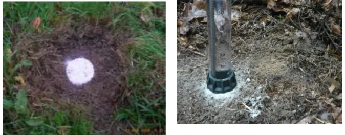
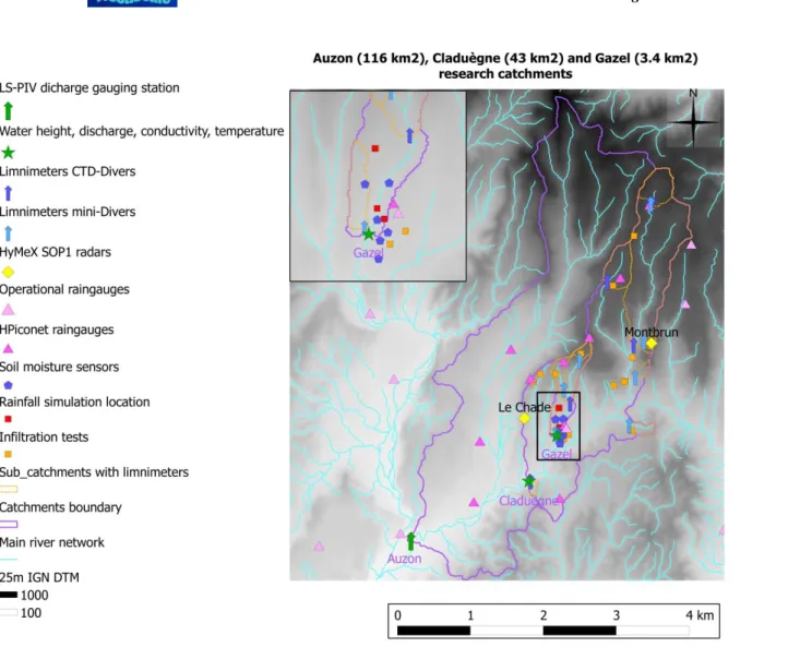
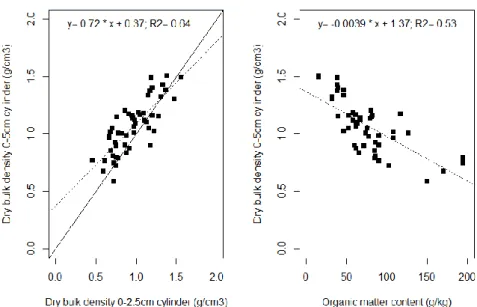
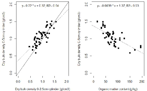
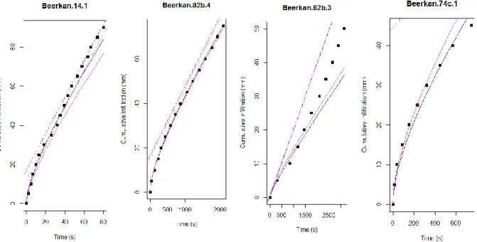
Figure 2-1 : (a) Photo of mini-disk infiltrometers (4.5 et 8 cm in diameter) (Photo Irstea) ; (b) Infiltrometer where the disk was removed from the tower from HSM (Photo C. Bouvier) ; (c) Infiltrometer used at LTHE (Photo I. Braud) ... 9 Figure 2-2: Setting up the sand layer. On the left, a layer of several mm thickness. On the right, a minimum thickness layer, but which probably extends too much beyond the cylinder. ... 10 Figure 2-3: Photos of the Beerkan experimental protocol. Left: undisturbed soil sampling to get initial soil moisture and dry bulk density. Middle: Filling of the cylinder with the plastic sheet before starting the infiltration test. Right: Measurement of the water level during infiltration. ... 12 Figure 3-1: Instrumentation of the Auzon catchment. The location of the infiltration test is shown as orange squares (From Braud et al., 2014). ... 15 Figure 4-1: Scheme of water front when the surface has a non zero slope where z is water height perpendicular to the topsoil surface, H is the water height within the infiltrometer and is the topsoil surface slope. ... 18 Figure 5-1: Location of the sampled points in the USDA textural triangle with different colors corresponding to land use (right) and soil typological unit (UC) (left) ... 29 Figure 5-2: Histogram of coarse fraction and organic matter content ... 30 Figure 5-3: Boxplot of dry bulk density (2.5 cm height cylinder) according to land use, UC soil class, geology and fraction of coarse fragments (see definition of classes in Table 5-1 ... 32 Figure 5-4: (Left) Comparison of dry bulk density measured using a small (2.5 cm height) and a large cylinder (5 cm height). (Right) Relationship between dry bulk density obtained with the 2.5 cm height cylinder and organic matter content ... 32 Figure 5-5 : Textural triangle where the data from the Claduègne infiltration tests are shown in red, and those from the Yzeron infiltration tests are shown in blue... 33 Figure 5-6: Correlation between dry bulk density obtained with the 2.5 cm height cylinders and organic matter for the data sets from Claduègne and Yzeron catchments ... 33 Figure 5-7: Examples of infiltration tests and of the fitted model using Eq. (50) for cumulative infiltration I (black) and infiltration flux q (pink). The dotted straight lines correspond to the equation for long times. (a) Point 14.1 with Tstab=40s. (a) Point 82b.4 with Tstab=1300s. (a)
Point 82b.3 with Tstab=300s. (a) Point 74c.1 with Tstab=2700s. ... 35
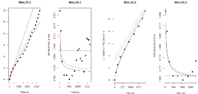
Figure 5-8: Example of a mini-disk infiltration test where acceleration of the flow was observed (left). Same infiltration test, after points selection (right). In this case a value of Ks=15 mm h-1 is obtained. The figure provides both the fit on cumulative infiltration (black)
and infiltration flux (pink). ... 36 Figure 5-9: Comparison of the results between Method 1 and Method 2 for the Beerkan infitltration tests for sorptivity, hydraulic conductivity, hg parameter and pore size radius m.
Parameters are fitted using the cumulative infiltration q. ... 37 Figure 5-10: Comparison of Method 1 results obtained when the optimization is performed on cumulative infiltration or on the infiltration flux for sorptivity, saturated hydraulic conductivity, hg parameter and pore size radius for the Beerkan infiltration tests. ... 37
Figure 5-11: Comparison of Method 1 results obtained when the optimization is performed on cumulative infiltration or on the infiltration flux for sorptivity, saturated hydraulic conductivity and pore size radius for the mini-disk infiltration tests. ... 38 Figure 5-12: Comparison of the mini-disk results between using the small (4.5 cm) and large (8 cm) diameter infiltrometers. The bottom left figure is a zoom of the bottom right one showing an outlier on the pore size radius. ... 39
Figure 5-13: Boxplot of the parameters obtained using the Beerkan and mini-disk for sorptivity, hydraulic conductivity and active pore size radius. The boxplot are drawn with 22 sample points where both an estimate of the Beerkan and mini-disk infiltrometers was available. ... 40 Figure 5-14: Boxplot of logarithm of saturated hydraulic conductivity derived from the Beerkan infiltration tests according to land use, UC soil class, geology and fraction of coarse fragments (see definition of classes in Table 5-1) ... 41 Figure 5-15: Illustration of the data processing when points are removed at the beginning of the infiltration test. ... 42 Figure 5-16: Analysis of mini-disk infiltration test using the DL-ST method. We first plot the cumulative infiltration as function of time (top left), the infiltration flux (top right) and the data in the (
t d
dI
, t ) space. Points in red are those selected for the DL regression line fit and the red line is the corresponding regression line. The full blue line is the regression line obtained when computing C1 and C2 from the L06 results and the blue dotted line is the long
term straight line provided by Eq. (69. Note that in this figure the points removed at the beginning of the infiltration test do not appear and the cumulative infiltration and infiltration time were modified (translation) before data analysis. ... 43 Figure 5-17: Same as Figure 5-16 but we have plotted all the points, including the first point which was removed (impact of sand layer). Even if the first point is not used in the regression (red points), the results are different than in Figure 5-16 because the value of I and t are different (no translation performed). With the DL-ST method, we get C1=0.415 and
C2=0.0121, leading to a negative value of K. ... 44
Figure 5-18: Comparison of the DL-ST and L06 method for the mini-disk infiltration tests. We show the comparison of S=C1 (top left), K (top right), (bottom left) and C2 (bottom
right) ... 45 Figure 5-19: Comparison of sorptivity (top) and C2 coefficient (bottom) obtained using the
DL method (black stars ± one standard deviation) and the L06 method (red crosses) for the mini-disk infiltration tests. ... 46 Figure 5-20: Comparison of the in situ saturated hydraulic conductivity derived from the Beerkan method (left) and the near saturation hydraulic conductivity K(-20mm) from the mini-disk (right) with the pedotransfer functions of Rawls and Brackensieck (1985) (RB85), Cosby et al. (1984) (C84) and Weynants et al. (2009) (W09) ... 48 Figure 5-21: Boxplot of dry bulk density with regards to DB land uses classes (top left), logarithm of saturated hydraulic conductivity (top right), hydraulic conductivity at -20 mm (bottom left) and pore size distribution diameters (bottom right) for the KS land uses classes ... 50 Figure 5-22: Boxplot of dry bulk density (top left), logarithm of saturated hydraulic conductivity (top right), hydraulic conductivity at -20 mm (bottom left) for two clay content classes (lower or higher than 45%). ... 51 Figure 5-23: Representative retention curves (left) and hydraulic conductivity curves (right) for the three combined DB and KS classes. ... 52
List of tables
Table 3-1: Main characteristics of the sampled fields. ... 14 Table 5-1: Number of sampled points according to various typologies for Beerkan and mini-disk infiltration tests. The total number of Beerkan points is 52 and of that of mini-mini-disk points is 38. ... 29 Table 5-2 : Statistics of the particle size data ... 31 Table 5-3: Statistics of dry bulk density (2.5 cm height cylinder), final water content and computed sortpivity, hydraulic conductivity and hg parameter for the Beerkan method and sorptivity, hydraulic conductivity for h=-20mm for mini-disk infiltrometers. Values indexed by _I were computed using cumulative infiltration and values indexed by _q using the infiltration flux. ... 40 Table 5-4 : Statistics of the results of the L06 and DL-ST methods on the mini-disk infiltration tests. Negative values were discarded from the analysis. ... 45 Table 5-5: Values of the estimated hydraulic conductivity for the various pressures using the LTHE infiltrometer. We also provide in blue the values obtained at the same points using the Beerkan method (h=0) and the mini-disk (h=-20mm) ... 47 Table 5-6: Values of statistics of the saturated hydraulic conductivity calculated using the various pedotransfer function and the Beerkan and mini-disk. Values are provided in mm s-1 ... 49 Table 5-7: Statistics of the soil hydraulic parameters (dry bulk density, saturated hydraulic conductivity, hydraulic conductivity at -20 mm, scale parameter hg of the retention curve,
pore size diameters ... 49 Table 5-8: Parameters of the representative retention curves and hydraulic conductivity curves for the three DB-KS classes ... 52
Abstract
In this report, we present the infiltration field campaign conducted in May-June 2012 in the 48 km2 Claduègne catchment (Ardèche, France). First we present the different measurement protocols using either simple ring infiltrometers (Beerkan method) or suction disk infiltrometers. Then the sampling strategy is presented.
The theoretical aspects of infiltration equations and different methods used in infiltration tests analysis are described in details. In particular, the BEST (Beerkan Estimation of Soil Transfer) method is used in the analysis of single ring infiltration data and mini-disk infiltrometer with a -20 mm suction. This method is compared to the differential linear, single (DL-ST) method, showing reasonable agreement, although systematic biases are evidenced. Multiple suction disk infiltrometers are analyzed using permanent regime equations.
The single ring infiltration tests provide estimates of the retention curve and hydraulic conductivity curves. The infiltrometers provide information about the hydraulic conductivity close to saturation. We present the statistical analysis of the results, which show that the soils have generally high hydraulic conductivity, especially in forested soils. Dry bulk density is also much lower in natural soils than in cultivated soils. In situ measurements are compared with three representative pedo-transfer functions showing poor capability of the latter in reproducing observations. On the other hand, land use is found more discriminant in determining soil hydraulic properties. The statistical analysis of the samples allows defining two classes for dry bulk density with significantly different values gathering respectively natural and cultivated soils. In terms of saturated hydraulic conductivity, two land uses classes gathering forested fields and moors on the one hand, and pasture and cultivated land on the other hand can be distinguished. This allows proposing a first strategy of soil hydraulic properties spatialization in the Claduègne catchment, by combining the dry bulk density and hydraulic conductivity classes in three main families of soil hydraulic properties, depending on land use.
Acknowledgements
The study was funded by the Agence Nationale de la Recherche (ANR) FloodScale project under contract ANR 2011 BS56 027.
Jean –Pierre Vandervaere is thanked for stimulating discussions during the data set analysis and provided most of the inputs related to the differential linear method.
The following persons are thanked for their contribution to the field campaign. Stanislas Bonnet performed the analyses for the choice of the sampled fields and he established the contact with all the owners. He also actively contributed to the Beerkan and mini-disk field campaigns as well as Flora Branger and Mickaël Lagouy. Olivier Vannier and Louise Jeandet performed the infiltration tests using the LTHE infiltrometer with multiple suctions and Louise Jeandet analyzed the data. Melissa Vuarant is also thanked for her contribution to data analysis.
During the field campaign, a new device, called saturometer was also tested. It was operated by Jean-Pierre Vandervaere, Olivier Vannier, Florent Blancho and later by Melissa Vuarant from Grenoble University.
We also thank all the field owners for allowing us to perform the infiltration tests in their fields.
This report describes the experimental methods used to perform infiltration tests in the Claduègne catchment (Ardèche, France) in May-June 2012, the sampling protocols and the methods used for the infiltration tests analysis. It provides a first view of the obtained results.
1. General objectives of the study
This study is part of the FloodScale1 project (Braud et al., 2014), dedicated to the observation and understanding of processes leading to flash floods in the Mediterranean context. More specifically, the study contributes to WP3.4 “Documentation and mapping of soil hydraulic properties, soil geometry and vegetation cover of small catchments”.
Indeed, in infiltration-excess prone areas, the saturated hydraulic conductivity is the key factor, which must be documented. The working hypothesis is that the pedology/texture/land use combination is more relevant for the spatialization of soil hydraulic properties than the traditional pedo-transfer functions based on texture and dry bulk density only (Gonzalez-Sosa et al., 2010; Calianno, 2010; Rault, 2010). In particular, we would like to document the impact of macropores in enhancing hydraulic conductivity close to saturation (e.g. Schwartz et al., 2003; Gonzalez-Sosa et al., 2010).
The study was conducted at the scale of a small to medium size catchment which is part of the FloodScale pilot site: the Claduègne catchment (48 km2), located in the Ardèche catchment. An infiltration test campaign was conducted in May-June 2012 to document the surface soil hydraulic properties using suction infiltrometers and positive head infiltration tests following the protocols proposed in Gonzalez-Sosa et al. (2010). Infiltration tests, using infiltrometers with multiple suctions were also performed at some locations.
This document presents the experimental protocols, the sampling strategy, as well as the methods used in the infiltration tests analysis. An analysis of the results is also conducted in order to assess the validity of the working hypothesis (largest impact of land use than soil texture on soil hydraulic properties) and to provide first recommendations for the spatialization of the surface soil hydraulic properties at the scale of the small catchments.
2. Protocols for infiltration tests
Two types of infiltration tests have been conducted: Infiltration tests based on suction-disk infiltrometers
Infiltration tests with a positive head using the Beerkan method (Braud et al., 2005) 2.1. Protocol for succion-disk infiltrometers
Several types of infiltrometers were available in the various research teams
Mini-disk infiltrometers (Sols Mesures with two diameters 4.5 and 8 cm) at Irstea-Lyon Villeurbanne (Figure 2-1a)
Infiltrometers where the disk was removed from the tower (model SW 080 B, SDEC) available at HSM (Figure 2-1b)
Infiltrometers according to Perroux and White (1988) at LTHE (Figure 2-1c)
Figure 2-1 : (a) Photo of mini-disk infiltrometers (4.5 et 8 cm in diameter) (Photo Irstea) ; (b) Infiltrometer where the disk was removed from the tower from HSM (Photo C. Bouvier) ; (c) Infiltrometer used at LTHE (Photo I. Braud)
2.1.1. Field equipment
In addition to the infiltrometers presented above, the following equipment are required:
GPS for getting the location of the infiltration test
Chronometer (accuracy 1 s)
Plastic can of about 20-30 l of water
An installation template with the same size as the infiltrometer
A flattening tool to get the surface plane, which can enter this template
Contact sand with grains as small as possible (Fontainebleau sand type with diameter 0.1/0.35 mm ; Hostun sand, diameter 150 µm used at LTHE)
Small cans for taking soil samples in order to get the initial soil moisture. If the cylinder volume is also known, it is possible to get the dry bulk density. At Irstea, we used cylinders with 4.3 cm and 2.5 cm height.
One cylinder of known volume for taking a soil sample in order to determine the dry bulk density. At Irstea, we used cylinders with 7.5 cm and 5 cm height. The dry bulk density is generally lower with the smaller cylinder as it samples more superficial layers. The accuracy of the dry bulk density is generally higher with the 5 cm height cylinder.
Plastic bags for taking soil samples (type freezing bags) used to get the particle size distribution
Auger for taking soil samples
2.1.2. Measurement protocol
Give a reference name to the infiltation test (field n°/test n°)
Take the position of the location using the GPS
Take off the vegetation and surface litter at the surface using a brush
Put a sand layer ensuring a good contact between the soil and the infiltrometer (Figure 2-2a). This sand layer must not extend beyond the cylinder (see recommendation in Vandervaere, 1995, p.32-332 and a bad example in Figure 2-2b). The thickness of this
2
« Cette couche [de sable] est aplanie au moyen d’une taloche. Le sable en excès dépassant la taille du disque doit impérativement être éliminée (en général juste après le début de l’essai) pour ne pas biaiser les résultats en
layer is discussed: at Irstea, we generally use the smallest thickness allowing getting a plane surface. At HSM a 1 cm thickness layer is used. This thickness is probably not critical when the permanent regime is analyzed, but is more important when transitory regime is also considered in the analysis.
Take a soil sample (500 g to 1 kg) and put it in the plastic bag for particle size distribution analysis
In a small can, take a soil sample (30 g) close to the infiltration site. Close the can, put a number. It will provide the initial soil moisture after 48 h soil drying in an oven at 105°C.
Fill the infiltrometer with water and choose the suction. In case of multi-suction infiltration tests, start with the lowest pressure and increase it to gradually approach saturation. It is possible to test the tightness of the infiltrometer by closing the air entry: the water must not go out.
Note the initial level in the infiltrometer on the field sheet
Start the infiltration test with very close readings. The field sheet of JP Vandervaere proposes 5, 10, 15, 20, 30 s. But if the infiltration is very rapid, it can be more convenient that one person provides the ruler readings to the operator with the chronometer who takes the corresponding times.
According to the infiltration speed, take a reading every 3 or 5 minutes.
If only one pressure is considered, take off the infiltrometer once the permanent regime has been apparently reached and take a soil sample in the wet surface to get the final soil moisture and the dry bulk density (use the largest cylinder of known volume). If several suctions are monitored, set the next suction and continue the infiltration test without moving the infiltrometer from the surface.
Perform three infiltration test per field sampling, if necessary at several levels along the slope
If a multiple suction infiltration test is conducted, the recommended pressures are -150, -100, -60, -25, -10 and -5 mm.
Figure 2-2: Setting up the sand layer. On the left, a layer of several mm thickness. On the right, a minimum thickness layer, but which probably extends too much beyond the cylinder.
augmentant le rayon effectif à la surface du sol. Pour pallier ce risque, on peut utiliser un gabarit constitué d’un anneau de garde dont le diamètre intérieur est égal à celui du disque. Cet anneau, dans lequel la taloche peut être insérée, est simplement posé à la surface du sol et le sable, versé à l’intérieur »
2.2. Protocol for the Beerkan infiltration tests
“Beerkan” infiltration tests or “single ring infiltrometer” are realized using a positive water head value at the soil surface, using cylinders, laid over the surface (with a minimal burying to avoid lateral leaks).
They allow, when complemented with other in situ measurements (see below), the estimation of the parameters of the retention and hydraulic conductivity curves useful for water transfer modelling in the soil (with for example the Richards equation).
The theoretical bases of the method, as well as the practical use are described in Braud et al. (2005) and Lassabatère et al. (2006). The experimental protocol is adapted from Gonzalez-Sosa et al. (2010) for the cylinders of large diameters, which allow, when the spatial variability is important, to get more representative results, given the larger sampled surface. For catchment scale modelling, it is recommended to select the files using topographical, land use and soil maps and to verify the accessibility of the sites. The sampled fields should have an area ranging between 10 m2 < S < 100 m2. Three locations, distributed randomly within the field (or sampling different levels along a slope) are selected to perform three replicates. Each location must be geo-referenced. When the area is larger, it is convenient to realize one additional test per 100 m2.
2.2.1. Field equipment
GPS for getting the location of the infiltration test
Cylinders of 400 mm x 250 mm, slightly cutting at the bottom
Hammers (about 1 kg)
Something allowing to hit on the cylinder in order to bury it as homogeneously as possible (like wooden beams)
Metallic rulers of about 20-30 cm with 1mm accuracy
Chronometer (accuracy 1 s)
Plastic can of about 20-30 l of water
Graduated buckets to measure the required water volume poured into the cylinder
Thermometer
Small cans for taking soil samples in order to get the initial soil moisture. If the cylinder volume is also known, it is possible to get the dry bulk density. At Irstea, we used cylinders with 4.3 cm and 2.5 cm height.
One cylinder of known volume for taking a soil sample in order to determine the dry bulk density. At Irstea, we used cylinders with 7.5 cm and 5 cm height. The dry bulk density is generally lower with the smaller cylinder as it samples more superficial layers. The accuracy on the dry bulk density is generally higher with the 5 cm height cylinder.
One square meter of plastic sheet
Plastic bags for taking soil samples (type freezing bags) used to get the particle size distribution
Auger for taking soil samples
2.2.2. Measurement protocol
Give a reference name to the infiltration test (field n°/test n°)
Take off the vegetation and surface litter at the surface using a brush
Take a soil sample (500 g to 1 kg) and put it in the plastic bag for particle size distribution analysis
In a small can, take a soil sample (30 g) close to the infiltration site (Figure 2-3a). Close the can, put a number. It will provide the initial soil moisture after 48 h soil drying in an oven at 105°C.
Insert carefully the cylinder into the soil in order to reduce the soil surface alteration by turning from right to left and from left to right
Put the wooden beams above the cylinder and hit it uniformly until the cylinder is buried in the soil (2 cm depth)
Put the plastic sheet within the cylinder so that the whole cylinder surface is covered
Pour a known water volume in the cylinder (2 to 12 l according to the cylinder size) and pour it in the cylinder above the plastic sheet. During the infiltration campaign in the Claduègne a 12 l water volume was used (Figure 2-3b).
Take the water temperature
Take off the plastic sheet rapidly but carefully to avoid overflowing water outside the cylinder
Measure the initial water level height and start the infiltration test with very close readings (Figure 2-3c). The field sheet of JP Vandervaere proposes 5, 10, 15, 20, 30 s. But if the infiltration is very rapid, it can be more convenient that one person provides the ruler readings to the operator with the chronometer who takes the corresponding times.
According to the infiltration speed, take a reading every 3 or 5 minutes.
Once all the water has infiltrated, take off the cylinder and take a soil sample in the wet surface to get the final soil moisture and the dry bulk density (use the largest cylinder of known volume).
Perform three infiltration test per field sampling, if necessary at several levels along the slope
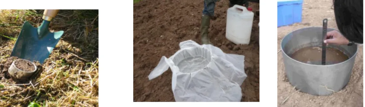
Figure 2-3: Photos of the Beerkan experimental protocol. Left: undisturbed soil sampling to get initial soil moisture and dry bulk density. Middle: Filling of the cylinder with the plastic sheet before starting the infiltration test. Right: Measurement of the water level during infiltration.
3. Sampling strategy
In order to test the working hypothesis (land use versus soil texture impact on soil hydraulic properties), the choosen sampled fields were selected in order to sample a maximum number of combinations of geology / pedology / land use.
The following GIS layers were used in the analysis (see details in Bonnet, 2012): - A 25 m Digital Elevation Model (DTM) from BDTopo IGN
- A pedology map from the Ardèche soil data base (Chambre d’Agriculture de l‘Ardèche) from the IGCS3
program with resolution 1/250 000.
- The geology map of the Auzon catchment from BRGM with resolution 1/25 000. - The 2006 Corine Land Cover map from IFEN4 with resolution 100 m
- The road network provided by BDTopo IGN - The land registry provided by BDTopo IGN
It was also tried to include a map characterizing the likelihood of surface runoff to occur (Bonnet, 2012) in the analysis, but this was leading to a too large number of combinations.
By overlaying the geology / pedology and land use maps a series of potential fields of interest were selected, taking into account their accessibility. The first selection was composed of combination including two types of geology: basalt and limestones; five land use classes: vineyards, pasture, forest, herbaceous, crops; and seven soil cartographic units from the pedology map, leading to 37 potential field locations.
A field survey was conducted at the beginning of May to confirm if the identified potential fields were similar to what was expected. The main source of differences was related to land use as the analysis was conducted with the 2006 Corine Land Cover map and the land use had sometimes changed in the meantime (building, abandonment of crops, etc.). After this field survey, the land registry was used to identify the field owners, who were contacted to obtain their agreement/refusal for sampling their fields.
Finally, a set of 18 fields was sampled through two field campaigns conducted between May 23-25 and June 18-19 2012. Table 3-1 provides the main characteristics of the sampled fields and the number of infiltration tests conducted in those fields (Beerkan, mini-disk infiltrometer with one suction, infiltrometer sampling using multiple suctions – in this case the used suctions are indicated).
The location of the fields is provided in Figure 3-1, together with the whole FloodScale instrumentation within the Auzon catchment.
3http://www.gissol.fr/programme/igcs/igcs.php
4
Field n° Land use Geology US Score for sensitivity to runoff production Beerkan Mini-disk 4.5 + 8 cm LTHE infiltrometer 3 Grassland (mowed alfafa) Basalt 64 2 3 2+1
5 Hedge of oaks Basalt 64 2 3 0
14 Natural grassland Limestones 33 2 3 2+1 -9, -4, -1.5, -1, -0.5cm
16 Coniferous forest Limestones 33 2 3 2+1 -10, -6, -4, -2, -0.7cm
17 Fallow land : moor and herbaceous
Limestones 33 3 3 2
22 Grassland grazed by sheeps
Basalt 65 1 3 2
25 Oak woods Basalt 65 0 3 2+1 -7, -4, -2, -1, -0.5cm +
-2cm
46 Grazed permanent
pasture
Limestones 26 1 3 2
46b Ploughed vineyard Limestones 26 1 3 1
52 Oak woods Limestones 29 2 4 2
58 Natural grassland Limestones 29 3 3 2
60 Fallow land : moor and herbaceous
Limestones 29 2 3 2
74a Moved ray grass
grassland Limestones 8 2 3 2+1 -7, -4, -2, -1, -0.5cm 74b Vineyard with herbaceous Limestones 8 2 4 2+2 -7, -4, -3, -1, -0.5cm 74C Grassland (mowed alfafa) Limestones 8 2 3 2+2 82b Vineyard Limestones 27 3 4 0 82t Grassland (mowed alfafa) Limestones 27 3 3 3
4. Analyses of the Beerkan and mini-disk infiltration tests
4.1. Theory of infiltration (permanent and transient regime)
The following description is taken from Gonzalez-Sosa and Braud (2009)
From the theory of infiltration proposed by Philip (1969), several methods have been proposed to estimate soil sorptivity and (near)-saturation hydraulic conductivity from disk infiltrometer data. The methods proposed by Zhang (1997), Vandervare et al. (2000a) and Smiles and Knight (1976) will be presented in this section. These methods are based on an approximation of the infiltration equation for short to medium time steps.
The axisymmetric infiltration equation (3D) can be described using the following approximation for transient flow, when the initial water content is such that the initial hydraulic conductivity is much smaller than the value corresponding to the pressure of the infiltrometer (Haverkamp et al., 1994).
t S t DtI (1)
where I is the cumulative infiltration per unit of area (m), t is time (s), and S is the capillary sorptivity (m s1/2) and D is given by:
0
2 3 2 i R S K D (2)with , a constant constrained to be 0<<1, R is the radius of the infiltrometer (m), i is the
initial water content and 0 is the final water content, and =0.75 (Smettem et al., 1994). In
the following, and in order to simplify notation, it will be assumed that S S
i,0
The introduction of the second right hand side term in Eq. (1) was necessary because the expression provided by the first right hand-side term is only valid for very short times, especially with axisymmetric infiltration. In practice, in the field, it was difficult to obtain enough data points of cumulative infiltration at short time steps for a reliable sorptivity estimation using only the short time approximation.
For simplicity, Eq. (1) is written as:
t C t C t I( ) 1 2 (3) with S C1 (4) and
0 2 2 3 2 i R S K C (5)The sorptivity is obtained using the expression proposed by Parlange (1975):
d D S S i i i, 2 2 ( ) 0 0 0
(6)The first method that was applied to obtain the sorptivity and hydraulic conductivity is the cumulative infiltration (CI) fitting proposed by Zhang (1997)
where
1 1 0 A C h S (7) 2 2 0) ( A C h K (8)For soils with the van Genuchten (1980) type retention function, the coefficients have the empirical form
0.15 0 0 25 . 0 0 5 . 0 1 9 . 1 3 exp ) ( 4 . 1 r h n b A i (9) and
0.91 0 0 1 . 0 2 9 . 1 92 . 2 exp ) 1 ( 65 . 11 r h n n A n1.9 (10)
0.91 0 0 1 . 0 2 9 . 1 5 . 7 exp ) 1 ( 65 . 11 r h n n A n1.9 (11) =1/hVG and n are van Genuchten parameters, r0 is the radius of the mini-disk infiltrometer,
h0 is the applied suction, 0 is the water content at h0, i is the initial water content, and b is a
parameter, with a representative value equal to 0.55 (Warrick and Broadbridge, 1992).
The second method, (DL) differentiation linearization, was proposed by Vandervare et al. (2000a, b). It is described by:
t C C t d dI 2 12 (12) where d t dI is approximated by i i i i t t I I t I t d dI 1 . 1 (i=1, np-1) (13)
where np is the number of data points, and the corresponding t is calculated as geometric
mean 2 / 1 1 ] [ ti ti t (i=1, np-1) (14)
The third method is based on Smiles and Knight (1976) linear fitting (CL) (cumulative linearization). The solved equation is obtained by dividing both sides of Eq. (3) by t
t C C t t I 2 1 (15)The advantage of Eqs. (12) and (15) is that they lead to a linear fitting, which is more robust than a quadratic fitting when the fitting is directly performed using Eq. (3).
These three methods can be applied to estimate the soil sorptivity and hydraulic conductivity at pressure h0, from a fitting of coefficients C1 and C2 in Eq. (3), (12) or (15). Then, sorptivity
is directly equal to C1 (Eq. [3]) and the conductivity is deduced from C2 = D by:
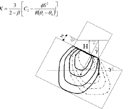
0 2 2 2 3 R i S C K (16)Figure 4-1: Scheme of water front when the surface has a non zero slope where z is water height perpendicular to the topsoil surface, H is the water height within the infiltrometer and is the topsoil surface slope.
The drawback of the methods that deduce hydraulic conductivity from Eq. (16) is that they can lead to negative values of the hydraulic conductivity which are not physical. However, this is also an advantage since it becomes the sign that the infiltration equation is not valid when another method will not provide negative values, thus leading to accept possible meaningless values. In fact, linearization methods are those that allow detecting validity problems of the infiltration equation; especially the DL method which eliminates the problem of the contact sand layer.
In the context of the experimental set up, the three methods are conditioned by the sand contact layer between the infiltrometer surface and the topsoil, organic matter content and sloping field surface. In our case the surface slope could affect the water flow and possibly also the measured infiltration.
According to Chen and Young (2006) vertical direction of the infiltration Ih on a sloping
surface is evaluated by the relation (see Figure 4-1)
cos 1 0 , , t I t I h h (17)This relationship establishes that the sloping surface increases the infiltration at small t by a factor of 1/cos which is the same result as the equation of Philip (1991), given the coordinate change. For t, or for large infiltration depths, the saturated hydraulic conductivity can be approximated as
h
st I
K (18)
In synthesis, the infiltration at short time is controlled by capillary forces, which would be independent of the slope angle for homogeneous and isotropic soils. However, increasing the slope angle increases the slope length, and increase the total infiltration volume. For large t (or large I), the controlling mechanism becomes the gravity, which would reduce the infiltration by a factor cos. This effect cancels with increasing slope length, and slope effect vanishes. Philip (1991) indicates that slope produces a maximum variation between horizontal and normal infiltration on sloping soil surface of about 13%. Variations are much smaller for small and moderate t values. The effect of slope was therefore neglected in subsequent analyses.
4.2. Analysis of permanent regimes
The following elements are translated from Vandervaere (1995) and correspond to the method used by HSM for the analysis of its infiltration tests, using permanent regime from infiltrometers.
Reynolds and Elrik (1991) and Ankeny et al. (1991) propose to determine the hydraulic conductivity from the Wooding (1968) solution, coupling fluxes obtained at the same location, using different water potential to determine K0 and 0.
Using the hypothesis of an exponential relationship between K and h (Gardner, 1958), the Kirchhoff potential has the following simple form:
i K K 0 0 (19)
where Ki << K0 if the soil is initially dry enough. Wooding (1968) analysis for a value h0 of
the soil water pressure, leads to the following expression:
r h K q s 4 1 exp 0 0 (20) Or in a logarithmic form: 0 0 4 1 ln ln h r K q s (21) With 𝐾𝑆= 𝐾𝑜𝑒𝑥𝑝(𝛼ℎ𝑜) (22)where the unknowns are Ks and . Equations (19) et (22) finally lead to:
0 0 0 0 exp 4 1 ln exp h r h q K (23)Reynolds and Elrick (1991) and Ankeny et al. (1991) propose to measure successively q0 at
two (or more) soil water pressures and to plot the (h0, lnq0) couples in a graph. The slope of
the straight line passing through two (or more) consecutive points leads to the values, while the intercept at h = 0 given by:
𝐼𝑛𝑡𝑒𝑟𝑐𝑒𝑝𝑡 = 𝑙𝑛 {𝐾𝑠(1 +𝜋𝑟𝛼4 )} (24)
allows the computation of Ks.
Practically, the successive qi values corresponding to values hi of the soil water pressure are obtained at the same location, which allows removing the effect of the spatial variability of soil properties. Soil water pressures values are applied in an increasing order, in order to avoid hysteresis impact. On the other hand, the method does not provide sorptivity values, as initial and final value of the soil water content cannot be measured for each infiltration step.
If Equation (21) is verified, successive points lnqi-hi should be located in a perfect straight line. However, in practice, this is seldom verified, which is equivalent to consider that is a function of h, and that the lnqi-hi couples do not belong to a unique straight line. Reynolds and Elrick (1991) and Ankeny et al. (1991) propose that K(h) is considered as a piece-wise exponential function. For two values of the soil water pressure, hi and hj (hi<hj), close enough to each other so that can be considered to have a unique constant value ij in the interval hij = [hi ; hj], Equation (21) can be written :
𝑙𝑛𝑞𝑖 = 𝑙𝑛 {𝐾𝑠(1 +𝜋𝑟𝛼4
𝑖𝑗)} + 𝛼𝑖𝑗ℎ𝑖 (25a)
𝑙𝑛𝑞𝑗 = 𝑙𝑛 {𝐾𝑠(1 +𝜋𝑟𝛼4
𝑖𝑗)} + 𝛼𝑖𝑗ℎ𝑗 (25b)
where Kij is a parameter having a physical meaning, only if hj = 0. In this case, Kij can be associated to Ks, the saturated hydraulic conductivity.
With this assumption, Equation (23) can be written:
r h h q h K m i ij m i 4 1 ln exp (26)with 2 j i m h h h
Given the hypotheses and, in particular the assumption that K(h) is a piece-wise exponential function, equations (25) and (26) are only valid in the hij interval if the following equalities are true :
ij ij
i j i j i j h q q K K exp (27)Where the ij coefficients are computed using:
ij i j ij h q q ln (28)
The mathematical developments of Ankeny et al. (1991) introduce the following approximation:
2 ij j i j j h h K h K h h (29)which is equivalent to a linearisation of the (h) function between hi and hj. The expression of ij proposed by Reynolds and Elrick (1991):
ij i j ij h K K ln (30) is replaced with
ij
i
j
i j j i ij i j ij q q h q q K K h K K 2 2 (31)Then, equation (20) becomes:
j i
i j i j i j i h h q q q q r q q r K 1 2 1 (32) which provides the value of the hydraulic conductivity for hm.This method was used for the interpretation of the infiltrometer tests performed by LTHE (last column of Table 3-1).
The theoretical background of the BEST (Beerkan Estimation of Soil Transfer) method is described in Braud et al. (2005) and its practical implementation is reported in Lassabatère et al. (2006). We will refer to the method as the L06 method in the following. The following description borrows lots of material from these two references, as well as from the work of Gonzalez-Sosa et Braud (2009).
In this approach, the aim is to determine the retention curve h(), relating the soil water pressure h (m) to the soil volumetric water content (m3 m-3); and the hydraulic conductivity curve K() relating the soil hydraulic conductivity K (m s-1) to the soil water content. The retention curve is modeled using the Van Genuchten (1980) approach (Eq. (33)) and the hydraulic conductivity using the Brooks and Corey (1964) model (Eq. (35)).
m n h h VG s 1 (33) with m k n 1 (34)
where s is the saturated water content (m3 m-3), hVG is a normalization parameter for the
water pressure, m and n are shape parameters and k is an integer chosen to be 1 (Mualem, 1976) or 2 (Burdine, 1953). In the following k=2 was used.
s s ) ( K K (35) where Ks (m s-1) is the saturated hydraulic conductivity and is a shape parameter related to
m and n by: p mn 2 2 (36) where p is a tortuosity parameter equal to 0 (Childs and Collis-George, 1950) or 1 (Mualem, 1976).
The objective is thus to derive, at each location, the values of the parameters of the retention and hydraulic conductivity curves, namely the shape parameters m, n and and the structure parameters s, hVG and Ks.
Two steps can be distinguished in the L06 method. The first one corresponds to the estimation of the shape parameters m, n and from soil texture. The second one is the optimisation of the infiltration tests in order to derive the structure parameters S, hVG and Ks. In the following,
it is assumed that s is available from field measurements, and, as mentioned before is
assumed to be equal to the measured final water content.
Estimation of shape parameters
Soil texture is derived from the particle-size distribution (< 2 mm), determined from a disturbed soil sample, and giving a curve with at least five fractions (clay, fine silt, coarse silt, fine sand, coarse sand). As a general rule, the more fractions that are determined, and the better is the curve fitting. The particle-size data provide the cumulative frequency distribution, F(d), as a function of particle diameter, d (m), to which the following curve is fitted
A B d d d F g 1 ) ( with B A1 2 (37)
where dg (m), is the normalization parameter for the particle diameter, and A and B are the
shape parameters of the curve. The quantities dg and B are optimized by least squares
techniques, stability of the convergence being achieved by using a change of variable x=1/d. The shape parameters m and n of the water retention curve can be derived from the knowledge of soil texture, and more specifically, from the knowledge of the A and B values. Following Haverkamp et al. (2005), we introduce soil specific shape indexes, pA, for the
particle-size distribution and, pm, for the water retention curve given respectively by:
A AB pA 1 (38) and m mn pm 1 (39)
where mn and AB are the products of the shape parameters of the retention and cumulative particle-size curves, respectively. They are related through
m A p p 1 (40) where s
s
s 1 2 1 2 (41)and s is the solution of the non-linear equation below given by Fuentes et al. (1998):
1
s 2s 1 (42)where is the soil porosity.
The derivation of the shape parameter for the hydraulic conductivity curve is performed using the classical capillary model of Eq.(36). In the following, the chosen value for the tortuosity parameter is 1 (Mualem, 1976).
Shape parameters of the water retention and hydraulic conductivity curves can therefore be derived from sole knowledge of soil texture.
Optimisation of the infiltration test and estimation of sorptivity and hydraulic conductivity The interpretation of infiltration tests using the L06 method starts from a more general infiltration equation than Eq.(1) and (2). Haverkamp et al. (1994) proposed an approximation of the full 3D infiltration equation for short to medium time steps, which reads:
K
K K
t R S t S t I i i i D 0 0 2 3 3 2 ) ( (43)where it is no more assumed that Ki K0 K
h0On the other hand, for long time steps, Haverkamp et al. (1994) show that the infiltration can be written (subscript 3D is omitted in the following for simplicity):
1 ln 1 2 0 2 0 2 0 i i K K S t R S K I (44)which corresponds to a linear variation with time.
Contrarily to the methods presented in section 4.1, which only exploit the short time steps behavior of the infiltration, the L06 method tries to take into account both short and long time
steps behavior. The parameter estimation can thus be based on more data than the approaches presented in section 4.1.
For long time steps, the infiltration flux is given by the slope of the curve I(t):
0 2 0 2 0 K AS R S K q i (45) with
0 i R A (46)The intercept of Eq.(44) is given by:
0 2 K S C b (47) with
1 ln 1 1 2 1 1 ln 1 1 2 1 0 0 i i K K C (48)which uses Eq.(35) such that:
0 0 i i K K (49)
Data for large time steps are used to fit Eq.(44) and thus derive estimates of q and b . For the interpretation of infiltration data at short times steps, two methods were tested:
i) Method 1: The first method follows the recommendations of Lassabatère et al. (2006) and consists in introducing Eq. (45) within Eq.(43), so that the only unknown becomes the sorptivity. This ensures a higher robustness of the optimization algorithm.
A B S Bq
t t S t I3D( ) 1 2 (50) with 0 0 0 0 1 3 2 1 3 2 i i i i K K K K B (51)ii) Method 2: The second method uses the intercept provided by Eq.(47) instead of the slope (Yilmaz et al., 2008). The latter is introduced within Eq.(43) and, once again, the expression only depends on the sorptivity, which can be optimized robustly. t S b BC A t S t I D 2 3 ( ) (52)
The optimization is performed by minimizing the sum of square errors between the simulated (using either Eq.(50) or (52)) and the measurements using k measured values, k being varied successively from 5 to np, the number of measurement points. The objective function is
written:
2 1 exp 2 ) ( ) , (
k i i i I t t I k S f (53)where ti, I(ti) are the measured values of infiltration as a function of time.
The optimization can also be performed using the infiltration flux data, where the infiltration flux is calculated as proposed by Lassabatère et al. (2006) (see their Eq. [18b]). Both methods were used in the following analysis.
The approximation provided by Eq.(43) is only valid for times ti lower than the gravity time
tgrav, which corresponds to the time at which gravity begins to dominate the flow process
(Philip, 1969): 2 0 K S tgrav (54)
Practically, Eq.(53) is optimized by varying k for about 5 to np and when the time is larger
than tgrav, i.e. for k=pI, the equation is no more valid. The value of the optimized parameter S2
for k=pI is thus the retained value.
Note that the data for k> pI are not lost, as they are used to fit Eq.(44) for longer times. In the
interpretation of the infiltration test, it means that Eq.(43) is valid for k smaller than pI. Then
Eq.(44) is valid.
The optimization process provides an estimate of the sorptivity S2. Then, an estimate of the hydraulic conductivity can be obtained using Eq.(45) (method 1) or Eq.(47) (method 2):
2 0 q AS K (55) b S C K 2 0 (56)
Note that, up to this step, the method can be applied both for infiltration test under suction or with a positive head. Thus it can be used for the interpretation of both the mini-disk and single ring infiltration tests.
As the saturated water content is estimated from the final and dry bulk density measurements, the last parameter which must be estimated to get all the parameters needed for the retention and hydraulic conductivity curves (Eqs. (33) and (35)) is the normalization parameter for the water pressure hVG. This is achieved using the definition of the sorptivity provided in Eq.(6).
The sorptivity can be rewritten as (Braud et al., 2005):
3 s i 1 0 i 1 2 s s i 1 s 0 i , , , 0 , , 0 , S S S S S S , (57)where the significance of the various terms is as follows.
1. The first term represents the integral given by Eq.(6) from 0 to s, i.e. over the
whole range of possible soil moisture content. It does not depend on initial and boundary conditions and can be considered as an integral soil characteristic.
2. The second term represents the influence of initial conditions.
3. The third term represents the influence of boundary conditions. When the surface head is positive, this term reduces to unity.
The first term of Eq.(57) can be calculated analytically for the combination of the van Genuchten retention model and the Brooks and Corey hydraulic conductivity model. This leads to:
s p_VG s s VG 2 , 0 c K h S , (58)where cp is a texture only dependent factor, the expression for which is given by Haverkamp
m m n m m m n m n c 1 1 1 1 p_VG , (59)where is the classical Gamma function.
Braud et al. (2005) propose an equation for estimating the sorptivity S
i,s
, which remains sufficiently accurate for the range 0/s<0.8 for sand and <0.9 for clay
s i s s i s s s i, 0, K K K S S . (60)Thus, when the surface head is positive or zero, the final water content is equal to the saturated water content (0 s) and Eq. (57) reduces to the first two terms. An estimate of hVG can be deduced as:
s i s i s VG p VG K c S h 1 _ 2 (61)When the surface head is negative as in the case of mini-disk infiltration test, we have no estimate of the third term of Eq. (57) and thus the infiltration test can no more be used to derive an estimate of hVG. However by estimating the water content corresponding to h=h0
using Eq.(33), it will be possible to verify if the hydraulic conductivity derived from the mini-disk fits the hydraulic conductivity curve given by Eq.(35).
It is also possible to obtain an estimate of the hydraulically active pore radius m, the expression of which can be found in Angulo-Jaramillo et al. (1996) and is derived from results of White and Sully (1987):
2 0 0 bS K K g i i w m (62)where =73 10-3 N m-1 is the surface tension, w=1000 kg m-3 is the water volumetric mass, g=9.81 m s-2 is the acceleration of gravity, b is a constant generally taken to be 0.55.
The L06 method was used for the interpretation of the Beerkan and mini- infiltrometer tests performed by Irstea (first columns of Table 4).
4.4. Analysis of transient regimes using the Differential Linearization (DL-ST) method The differentiation linearization (DL) , was proposed by Vandervare et al. (2000a, b). It is described by: t C C t d dI 2 12 (63)
In Vandervaere et al. (2000a) it is proposed to approximate d t
dI
i i i i t t I I t I t d dI 1 . 1 (i=1, np-1) (64)
where np is the number of data points, and the corresponding t is calculated as geometric
mean 2 / 1 1 ] [ ti ti t (i=1, np-1) (65)
However, if we assume that Eq. (3) is valid, we can write Eq. (63) as follows:
* 2 1 1 2 1 1 1 1 1 1 2 1 1 1 1 2 1 1 1 1 1 2 2 2 1 i i i i i i i i i i i i i i i i i i i i i i i i i i i t C C t t C C t t I I t t t t t t C C t t I I t t C t t C t t t t I I (66) where 2 1 * i i i t t t (67) The derivative is therefore associated to the arithmetic mean of the square root of time. In the following the DL method was applied with this minor modification.The DL method consists in adjusting Eq. (62) by linear regression fitting. However, the DL method is only a method to determine the values of the two parameters in Eq. (3) without bias. The second step which consists in determining S and K using the C1 and C2 values can
be achieved by different methods described in Vandervaere et al. (2000b) depending on the number of disk radii and pressure head values applied (see ST, MR, MS1 and MS2 methods in this paper). Although not always recommended by these authors, as only one infiltration test with one radius and one pressure was available, it is only the Single Test (ST) method which will be combined with the DL method in the following, what will be written DL-ST method. The sorptivity S = C1 is therefore provided by the intercept with the origin and the
hydraulic conductivity can be deduced from the slope of the regression 2C2 as follows.
i i i K R S C K K 0 2 2 2 3 (68)This method was used for the analysis of the mini-disk infiltrometers performed by Irstea. 4.5. Comparison of the L06 and DL-ST methods
Both DL-ST and L06 methods use the same basic equations for short to intermediate times. The difference is that the parameters optimization is performed in the (I,t) space for L06
whereas the (
t d
dI
, t ) space is used for DL method. In addition, the DL method only uses short to medium times for the optimization, whereas the L06 method also exploits long times. Nevertheless, it is expected that the parameters values optimized using the L06 method lead to consistent (
t d
dI
, t ) space. In particular, for long times, the points should verify:
AS K
t t d dI 0 2 2 (69) It means that the points for long times should be aligned on a straight line, with a slope different to the one at short time steps and this straight line goes through the origin.This property will be used to compare the results of the L06 and DL-ST methods in the following.
5. Results
5.1. Distribution of the sample points, texture and particle size distribution
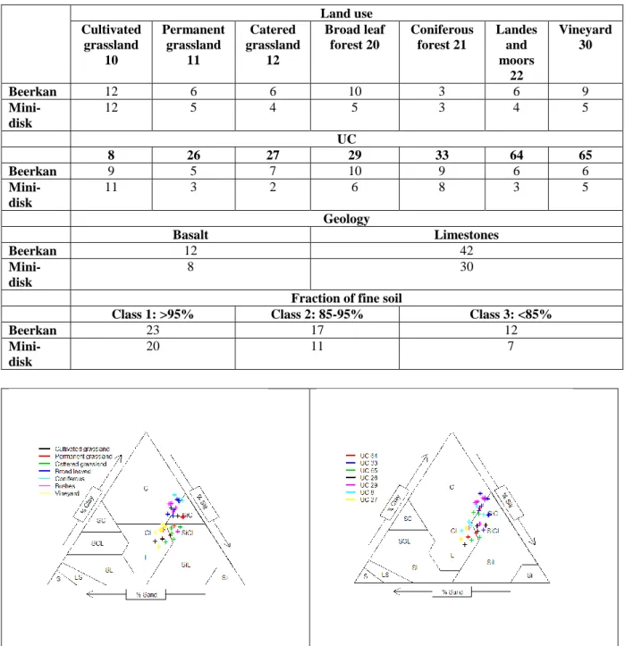
In order to analyze the sampled points, they can be classified according to various factors. The following were considered: land use, soil cartographic unit UC, geology, fraction of coarse fragments. The points’ distribution according to those criteria is provided in Table 5-1, showing that the sampling is not homogeneous amongst classes.
Table 5-1: Number of sampled points according to various typologies for Beerkan and mini-disk infiltration tests. The total number of Beerkan points is 52 and of that of mini-disk points is 38.
Land use Cultivated grassland 10 Permanent grassland 11 Catered grassland 12 Broad leaf forest 20 Coniferous forest 21 Landes and moors 22 Vineyard 30 Beerkan 12 6 6 10 3 6 9 Mini-disk 12 5 4 5 3 4 5 UC 8 26 27 29 33 64 65 Beerkan 9 5 7 10 9 6 6 Mini-disk 11 3 2 6 8 3 5 Geology Basalt Limestones Beerkan 12 42 Mini-disk 8 30
Fraction of fine soil
Class 1: >95% Class 2: 85-95% Class 3: <85%
Beerkan 23 17 12
Mini-disk
20 11 7
Figure 5-1: Location of the sampled points in the USDA textural triangle with different colors corresponding to land use (right) and soil typological unit (UC) (left)
The soil class of the sampled points is plotted in the USDA triangle in Figure 5-1 for the various land uses and soil mapping units (UC) of the BD-Sol Ardèche soil data base.
Figure 5-1 shows that soil texture in the Claduègne catchment is mostly composed of clay, clay loam, silty clay loam and silty clay, with one point located in the loam class. Figure 5-1a also shows that sample points located in broad leaf forests, coniferous forests and to a lesser extend bushes are located in the finer soils: clay and silty clay. It may be related to the fact that those soils are less favorable to agriculture.
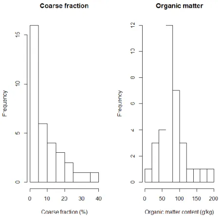
Figure 5-2: Histogram of coarse fraction and organic matter content
Table 5-2 provides the statistics of the particle size data, coarse fragments and organic matter contents of the sample points (34 points). The table also provides the shape parameters of the retention and hydraulic conductivity curves presented in section 4.3 (Eqs. (33) to (42)). Figure 5-2 provides histograms of coarse fraction (sum of gravels and stones) and of organic matter contents over the whole sample.
As already visible on the textural triangle, the sampled soils have a high fraction of clay and a low fraction of sand. We also note that more than 50% of the points have coarse fraction lower than 5%, but it can reach values as high as 40% (Figure 5-2-left). Organic content is high (Figure 5-2-right) in forests and bushes and the value is significantly larger than in cultivated points (value of the Kruskal-Wallis test is p=0.0033).
In terms of shape parameters of the retention curve, the n parameter has a very low range, with a CV of 1%. The shape parameter of the hydraulic conductivity curve has a larger variability amongst soils with a CV of 18%. Note also that the median value of is large (25.17) which is consistent with the high clay content. This also means that the hydraulic conductivity decreases very rapidly from saturation.
According to the Kolmogorov-Smirnov test, the hypothesis of normal distribution cannot be rejected at the 5% level, except for the dg parameter.