HAL Id: hal-01790280
https://hal.archives-ouvertes.fr/hal-01790280
Submitted on 11 May 2018
HAL is a multi-disciplinary open access
archive for the deposit and dissemination of
sci-entific research documents, whether they are
pub-lished or not. The documents may come from
teaching and research institutions in France or
abroad, or from public or private research centers.
L’archive ouverte pluridisciplinaire HAL, est
destinée au dépôt et à la diffusion de documents
scientifiques de niveau recherche, publiés ou non,
émanant des établissements d’enseignement et de
recherche français ou étrangers, des laboratoires
publics ou privés.
MAC Mechanism for a Scalable Wireless Sensor
Networks using Independent Duty Cycles
Affoua Thérèse Aby, Alexandre Guitton, Michel Misson
To cite this version:
Affoua Thérèse Aby, Alexandre Guitton, Michel Misson. MAC Mechanism for a Scalable Wireless
Sensor Networks using Independent Duty Cycles. NICST (International France-China Workshop on
New and Smart Information Communication Science and Technology to Support Sustainable
Devel-opment), 2013, Chine, China. �hal-01790280�
MAC Mechanism for a Scalable Wireless Sensor
Networks using Independent Duty Cycles
Affoua Th´er`ese Aby
(1,2), Alexandre Guitton
(3,2), Michel Misson
(1,2)(1) Clermont Universit´e, Universit´e d’Auvergne, LIMOS, BP 10448, F-63000 Clermont-Ferrand, France (2) CNRS, UMR 6158, LIMOS, F-63175 Aubi`ere, France
(3) Clermont Universit´e, Universit´e Blaise Pascal, LIMOS, BP 10448, F-63000 Clermont-Ferrand, France Emails:{aby,guitton,misson}@sancy.univ-bpclermont.fr
Abstract—Wireless sensor networks (WSNs) are increasingly
used in order to monitor the environment. It is important to ensure that protocols for WSNs are scalable (as WSNs can be composed of hundreds of devices) and energy-efficient (as they are designed to operate for years). In this paper, we show that in synchronized MAC protocols, synchronization requires a lot of energy, and in unsynchronized MAC protocols, it is difficult for neighbor nodes to communicate together in an energy-efficient manner (as they are not synchronized). We use a mathematical model to quantify the average communication delay for unsynchronized MAC protocols, and to compute the average probability that this delay is infinite. Then, we propose a distributed MAC mechanism, based on the beacon-enabled mode of IEEE 802.15.4, without the synchronization mechanism. Our mechanism greatly reduces the probability that the com-munication delay is infinite, allows nodes to communicate with their neighbors periodically (but not systematically), and ensures that the energy consumption is constant. Finally, we evaluate the performance of our mechanism by simulation, and conclude that it can be integrated into a scalable MAC protocol.
I. INTRODUCTION
Wireless sensor networks (WSNs) are composed of cheap devices that can sense the environment, perform some com-putations, and communicate together using wireless links. These advantages allow them to be used to monitor various environments, such as volcanoes [1], bridges [2], fields [3], and bird nests [4]. These applications often require a large number of network devices, and they have to run for a long period (usually, several years).
The IEEE 802.15.4 standard [5] has been proposed to enable low-power communications in personal area networks, including wireless sensor networks. It has two operational modes: the non beacon-enabled mode and the beacon-enabled mode. In the non beacon-enabled mode, most devices wake up only when they have data to transmit, and go back to sleep afterwards. This requires some devices to always remain awake in order to receive data, which consumes a lot of energy. In the beacon-enabled mode, all devices are synchronized: they all wake up at the same time in order to communicate, and go back to sleep at the same time in order to save energy. However, the synchronization of devices is often difficult to achieve, and does not scale well.
In this paper, we propose a distributed MAC mechanism for WSNs which aims at improving the connectivity and the scalability of the IEEE 802.15.4 standard, while having
a low energy consumption. Our mechanism is to remove the synchronization constraint of the IEEE 802.15.4 beacon-enabled mode by having devices use independent duty cy-cles. Our approach improves the connectivity as devices will eventually (with high probability) share a common activity period and be able to communicate, even though they are not synchronized. Similarly, our approach improves the scalability as synchronization is no longer necessary when nodes wake up. Note that our mechanism can be used as an essential building block of a MAC protocol.
The paper is organized as follows. Section II gives a detailed explanation of the IEEE 802.15.4 standard, which is the basis of this work. Section III presents how independent duty cycles can improve the connectivity and scalability of the network. Section IV describes our simulation results, and shows that we are able to achieve a similar energy efficiency as IEEE 802.15.4. Section V discusses how our proposition can be implemented as a distributed mechanism. Finally, Section VI summarizes our work.
II. STATE OF THE ART
Most energy-efficient MAC protocols are based on a peri-odic sequence of activities and inactivities, called duty cycle. Nodes communicate during the activity period, and can sleep during the inactivity period, which spares energy. Those MAC protocols can be divided into two categories, depending on whether they are synchronized or not.
A. Synchronized MAC protocols
The IEEE 802.15.4 protocol [5] in beacon-enabled mode is one of the most common energy-efficient MAC protocols. Each full-function device (FFD) sends a beacon regularly, with a period called BI (for beacon interval). When a
reduced-function device (RFD) receives a beacon, it starts its activity period for a duration called SD (for superframe duration).
The ratio SD/BI defines the duty cycle of the protocol.
Note that all nodes share the same activity period, as they are synchronized by the beacon reception. The medium is accessed using the slotted CSMA/CA (carrier-sense multiple access with collision avoidance) algorithm.
In D-MAC [6], nodes are synchronized according to their depth on a collection tree. When nodes of depth d are in a
slot. In Z-MAC [7], a TDMA (time-division multiple access) approach is used to synchronize nodes. A slot is assigned to all nodes in the configuration phase, and is used in case of high contention. In case of low contention, all nodes access the channel simultaneously, with a contention access mechanism. In G-MAC [8], time is divided into three periods: a collection period (where the medium is accessed by CSMA/CA), a period of traffic indication (whose role is to maintain synchronization between nodes) and a distribution period (where the medium is accessed by TDMA). All nodes have simultaneous activities during the first and the second periods, and non-simultaneous activities during the third period. In S-MAC [9], each node propagates periodically its time schedule to its neighbors. Each node adapts its activity to the first schedule it receives. Thus, nodes can determine when to be active or inactive, depending on whether they have to communicate with a given neighbor or not. In [10], the authors show that higher performance can be achieved when different wireless personal area net-works have disjoint activity periods. However, ensuring that activity periods are disjoint requires synchronization. In MC-LMAC [11] nodes are synchronized but, use multiple channels dynamically. MC-LMAC is based on the single-channel proto-col LMAC [12]. MC-LMAC maximizes throughput of LMAC by using a plurality of channels for transmission. The principle in MC-LMAC is as follows, firstly, nodes try to find time slots following the rule of LMAC. Second, the nodes that have not been able to find time slots invite their free neighbors to listen on an agreed channel. The problem with MC-LMAC is that most of the difficulties of synchronizing all MAC protocols duty cycle synchronous, dynamic scheduling interface change requires the generation of a large number of control message.
B. Not-synchronized MAC protocols
The IEEE 802.15.4 protocol in non beacon-enabled mode allows nodes to communicate without requiring a synchro-nization mechanism. When an RFD has to send data to an FFD, it simply wakes up and transmits the data. This requires, however, the FFDs to be active all the time, which con-sumes energy. The medium is accessed using the non-slotted CSMA/CA algorithm. Although the non beacon-enabled mode allows nodes to have non-simultaneous activities, it cannot be used in practice due to its energy requirements.
In B-MAC [13], nodes are not synchronized but wake up periodically for a short duration. When a sender node has to communicate to a receiver node, the sender node sends a long preamble before its frame (which makes B-MAC a sender-initiated protocol). When the receiver wakes up, it detects the preamble and stays active until the end of the preamble and the reception of the frame. While this approach yields good performance, nodes have to stay awake frequently in order to receive frames, and therefore the energy consumption of B-MAC relies heavily on the traffic. In X-MAC [14], the same approach as B-X-MAC is used. Instead of using a long preamble, each sender sends several small frames, which allows the receiver to go back to sleep as soon as it has received the frame, rather than having to wait for the
preamble. WiseMAC [15], RI-MAC [16], ADB [17], PW-MAC [18], and EM-PW-MAC [19] focus on a receiver-initiated approach. In WiseMAC, preambles are used, but their lengths is reduced by allowing the sender to wake up before the beginning of the activity period of the receiver. In RI-MAC, the receiver initiates the communication. RI-MAC is based on low power probing, where the receiver sends a beacon to express its ability to receive data packets. RI-MAC reduces channel occupation (as it does not require nodes to send preambles), but generates high energy consumption. The same authors proposed the protocol ADB, to provide essentially a broadcast service in RI-MAC protocol. And PW-MAC for reduce the listening time of the sender in RI-MAC, by having each node compute its awakening times according to a pseudo-random number generator rather than according to a fixed schedule. The drawback of PW-MAC is that sending the beacons before packet transmission generates overhead, and introduces a delay when listening the channel. As PW-MAC in EM-MAC, a node computing its moments of awakening using a pseudo-random generator. A node independently decides its wake-up time and exchange channel. The wake-up channel is not necessarily the same as the channel for exchanging data. In EM-MAC, the sender also knows the parameters of the pseudo-random generator and receiver wake-up channel. EM-MAC inherits the shortcomings of PW-MAC, and more, in EM-MAC, each node invokes twice a pseudo-random generator, hence, generation of additional overhead.
III. IMPROVING THE ENERGY EFFICIENCY OF A LOW DUTY CYCLEMACPROTOCOL
We identified two main issues in IEEE 802.15.4. First, when the non beacon-enabled mode is used, several nodes cannot sleep and the energy consumption is high. Second, when the beacon-enabled mode is used, the required synchronization is difficult to achieve for a large number of nodes, and the fact that all nodes share the same activity cycle reduces the performance of the MAC protocol (since they all compete for the medium at the same time).
In the following, we show additional drawbacks of the existing approaches. Even in the case where nodes start their activity at different times (which increases the performance of the MAC protocol), some nodes might never have a shared activity, which is detrimental for the network. We also study the delay a node has to wait, on average, to meet another node.
A. Study of the probability of shared activities
Let us suppose that nodes have the same beacon interval but start randomly within the beacon interval. Let us denote byni each node,BI the duration of the beacon interval, and
α ∈ [0; 1] the duty cycle (that is, each node is active during SD = α.BI). Without loss of generality, we can assume that n1 starts at the beginning of its beacon interval (in this case,
n1 finishes its activity atα.BI).
First, we compute the probabilityPdisjoint thatn1 andn2 have disjoint activities. If α > 1/2, Pdisjoint = 0 as nodes are active during more than half of their beacon interval. Let
us now consider that α ≤ 1/2. Pdisjoint is equal to the probability thatn2starts its activity duration aftern1 finishes its own, and that n2 finishes its activity duration before n1 starts its next one. Thus,Pdisjoint is the probability that n2 starts in[α.BI; BI − α.BI[. This interval always exists since α ≤ 1/2 yields to α.BI ≤ BI − α.BI. As we assume
that the starting time of n2 is uniformly distributed, we have
Pdisjoint = (BI −2α.BI)/BI, that is Pdisjoint = 1−2α. For
instance, when α = 1/4, Pdisjoint = 1 − 1/2 = 1/2. When
α = 1/8, Pdisjoint = 1 − 1/4 = 3/4. When the duty cycle
is low, the probability that some nodes never share a common activity is high, which is an important drawback of existing methods.
Second, we compute the probabilityPall that there is a time
whenn nodes are active simultaneously. Recall that all nodes
have activity periods starting randomly (except forn1). Since these activities are independently chosen, we can computePall as Pall= Y i P (ni is active) = Y i α = αn.
For instance, whenα = 1/2 and n = 3, Pall = 1/8. When
α = 1/2 and n = 4, Pall = 1/16. It can be seen that when the
number of nodesn is large, the probability that all nodes share
a common activity is very low, which is also an important drawback of existing methods.
B. Study of the delay before a shared activity
It is important to know the delay before two nodes can have a shared activity, in addition to knowing that they will eventually meet. We define the average delay between two nodesn1 andn2 as the average duration between any instant when n1 is active, and the first instant when n1 andn2 are active. Note that sometimes, n1 and n2 never meet: these cases are not taken into account in the average delay, but the probability that this occurs isPdisjoint.
To compute the average delay, we examine two cases that are equally likely to occur. Case 1 is when n2 starts within[0; α.BI[, and Case 2 is when n2 starts within [BI −
α.BI; BI[. These two cases are depicted on Fig. 1. Notice
that it is not possible for n2 to start at other times, as this would cause an infinite delay.
noden1 noden1 noden2 noden2 x x y y (Case 1) (Case 2)
Figure 1. Two cases that can occur when two nodes n1and n2meet. Letd1 be the average delay for Case 1. Let us denote byx the instant within the activity of n1 (over which the average is performed), and byy the starting time of n2. According to
Fig. 1, we have: d1 = 1 α2.BI2 α.BI X y=0 y−1 X x=0 (y − x) + α.BI−1 X x=y 0 ! = (α.BI + 1)(α.BI + 2) 6α.BI .
Let d2 be the average delay for Case 2. Again, according to Fig. 1, we have: d2 = 1 α2.BI2 BI−1 X y=BI−α.BI y+α.BI−BI X x=0 0 + α.BI−1 X x=y+α.BI−BI (BI − x) = −α(2α − 3).BI 2 − 3.BI − 2 6α.BI .
The average delay d is thus: d =d1+ d2
2 =
(α.BI + 1).(4 + 3.BI − α.BI)
12α.BI . 64 128 192 256 0.0625 0.125 0.25 0.5 10 20 30 40 50 60 70
Delay (in seconds)
BI (in seconds) alpha
Delay (in seconds)
Figure 2. Numerical value of the delay d as a function of BI and α.
Figure 2 shows the delay d as a function of BI and α. It
can be noticed that even when the delay is not infinite, the delay is relatively large. It reaches up to 70 s for BI = 256
andα = 6.25%.
C. Description of our proposition
Our proposition can be summarized by the following items: • allowing nodes to start their activity at a random time
within the beacon interval,
• forcing nodes to have different beacon intervals while maintaining a given duty cycle,
• removing the constraint that all the nodes of the network have to agree on when to send their beacons.
The first item ensures that all nodes are not always ac-tive simultaneously, which improves the performance of the MAC protocol. The second item ensures that nodes have a high probability to meet while maintaining the same energy-efficiency as the beacon-enabled mode. The third item allows our mechanism to be independent of the number of nodes in the network, which enables its integration into a scalable MAC protocol. In this way, our proposition benefits from the energy-efficiency of the beacon-enabled mode (as each node keeps the
same duty cycle), without having the drawbacks of a global synchronization (as each node keeps its own time schedule).
Figure 3 shows the activities of three nodes as a function of time, with a duty cycle of 25% and when nodes start their activities randomly within the beacon interval. To ease the description, we made two simplifying assumptions: there are only 8 backoff periods per cycle (that is, BI = 8), and
the backoff periods are synchronized for all the nodes. In general, the number of backoff periods per cycle is much larger: for a beacon interval of26× 15.36 ms, which is about one second, there are 3072 backoff periods of 320µs each.
Backoff periods cannot be synchronized for all the nodes when there is no global synchronization, but the desynchronization only impacts one backoff period at most, out of all the backoff periods of the beacon interval. Periodically, nodesn1 andn2 share a common activity period (at the end of the activity ofn1 and at the beginning of the activity ofn2). However, in the example depicted here,n3never shares a common activity with neithern1norn2.
noden1 noden2 noden3 BI BI BI
Figure 3. Activities of three nodes as a function of time, with a duty cycle of 25%, and when activities start randomly within the beacon interval. Node
n3never shares a common activity period with n1nor n2.
Figure 4 shows the activities of three nodes as a function of time, for our proposition. Notice that for each node, the duty cycle is 25% (even if the beacon interval is different). Common activities between two nodes are no longer periodic: they appear depending on the beacon interval of each node. For instance,n1shares a common activity withn2at the beginning of the first activity period of n1, and at the end of its third activity period. Noden3 shares a common activity withn2 at the beginning of its first activity period, and a common activity with bothn1andn2 at the end of its second activity period.
noden1 noden2 noden3 BI1 BI2 BI3
Figure 4. Activities of three nodes as a function of time, with a duty cycle of 25%, for our proposition. All possibilities of shared activities (n1and n2, n1 and n3, n2 and n3, and all three nodes together) happen in this short
example.
The main advantages of our proposition are the following: • it does not require synchronization,
• the duration of the activity period is never exceeded,
• the probability that a node is isolated from the other nodes in range is low (see Pdisjoint),
• as few nodes are active simultaneously on average, contention access MAC protocols can achieve higher performance,
• there are times when all nodes are active, which enables to broadcast frames efficiently.
IV. SIMULATION RESULTS
In order to evaluate the performance of our proposition, we ran some simulations using a set of Perl scripts. As a basis for our comparison, we use a model similar to the one depicted on Fig. 3: BI has a constant value of 128 backoff
periods, and each node chooses randomly the beginning of its activity within the period. Our proposition, depicted on Fig. 4, allocates a random BI to each node, such that each BI is
within[64; 256] and is a multiple of 4. The activity duration in
our case varies for each node, but the duty cycle is constant for all nodes. Again, each node chooses randomly the beginning of its activity within its period. Each simulation lasts until a global periodicity is obtained (which happens after a number of backoff periods equal to the least common multiple of all theBIs). Note that all nodes are in range (that is, they are in
the same cell). In the following plots, each point is averaged over 500 repetitions.
Figure 5 shows the average probability for all the nodes of a cell to be active simultaneously, as a function of the number of nodes. We evaluate two duty cycles: 50% and 25%, and we compare the probability whenBIs are constant
(which is denoted by BI is not random) and when BIs are
different for each node (which is denoted by BI is random).
For a given duty cycle, the probability that all nodes are active simultaneously decreases with the number of nodes, as expected. However, whenBIs are random, the probability
is much higher than when BIs are constant, and decreases
linearly instead of exponentially. In all cases, our proposition yields a much higher probability than the state of the art. For instance, when the duty cycle is equal to 50% and for four nodes in a cell, the probability that they have a common activity is only 5% (out of active duration of nodes, which is only 50% of the time) when BIs are the same, while it
exceeds 40% when BIs are random.
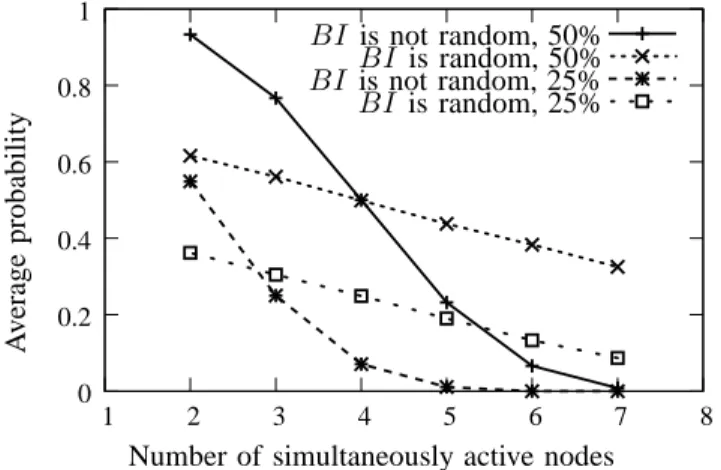
Figure 6 shows the average probability for several nodes in a cell to be active simultaneously, when the total number of nodes in the cell is seven. For instance, the probability that three nodes (out of seven) are active simultaneously for a duty cycle of 50% is about 60% whenBIs are constant, and about
80% when BIs are random. The probability that six nodes
(out of seven) are active simultaneously for a duty cycle of 50% is about 10% when BIs are constant, and about 40%
when BIs are random. With our proposition, the probability
that several nodes are active simultaneously decreases slowly. Figure 7 shows the average delay (in backoff periods) as a function of the number of nodes in the cell. We compute here only the delay until two nodes are active simultaneously, without considering the MAC delay required for two active
0 0.1 0.2 0.3 0.4 0.5 0.6 1 2 3 4 5 6 7 8
Number of simultaneously active nodes
A v er ag e p ro b ab il it y BI is not random, 50% BI is random, 50% BI is not random, 25% BI is random, 25%
Figure 5. Average probability for all nodes in a cell to be active simultane-ously. When BI is chosen randomly for each node, the probability that all nodes in a cell are active simultaneously at a given time is high and decreases slowly. 0 0.2 0.4 0.6 0.8 1 1 2 3 4 5 6 7 8
Number of simultaneously active nodes
A v er ag e p ro b ab il it y BI is not random, 50% BI is random, 50% BI is not random, 25% BI is random, 25%
Figure 6. Average probability for several nodes to be active simultaneously, for a total of seven nodes in a cell. When BI is chosen randomly for each node, the probability that several nodes are active simultaneously decreases slowly with the number of active nodes.
nodes to communicate. The delay is averaged over all pairs of nodes, but does not take into account the infinite values. Notice that the percentage of infinite delays is very high when BI
is not random, and very low whenBI is random. For a duty
cycle of 50%, the percentage of infinite delays varies between 0.5% and 1% whenBI is not random, and is always 0% when BI is random (for our 500 repetitions). For a duty cycle of
25%, the percentage of infinite delays varies between 50% and 51% whenBI is not random (which is very high), and varies
between 1.5% and 2% when BI is random (which is very
low). WhenBI is constant and the duty cycle is low, a large
number of delays are infinite and are therefore omitted from the computation. When BIs are random, the delay is higher
on average but only a small percentage of infinite delays are omitted.
V. IMPLEMENTATION AS A DISTRIBUTED PROTOCOL
In this section, we describe how to build a distributed and scalable protocol from our proposition.
0 50 100 150 200 250 300 350 400 1 2 3 4 5
Number of nodes in the cell
A v er ag e d el ay (i n b ac k o ff p er io d s) BI is not random, 50% BI is random, 50% BI is not random, 25% BI is random, 25%
Figure 7. Average delay for two nodes in a cell to be active simultaneously. When BI is chosen randomly for each node, the average delay is approx-imately twice higher than when BI is not random. However, when BI is chosen randomly, the probability that delays are infinite is very low.
Algorithm 1 presents our protocol. Note that all nodes share the following values:∆ is a duration (generally large), BIs are
chosen randomly within[minBI; maxBI], and dutyCycle is
the fixed duty cycle for each node. We assume here that nodes start randomly and independently. Initially, each node chooses its ownBI in [minBI; maxBI] according to our proposition,
and operates according to this BI. After ∆ backoff periods,
the node determines whether it has met any neighbor or not. If it has not, it draws a new BI and starts again. Otherwise,
it keeps the same value forBI.
Algorithm 1 Scalable protocol using independent duty cycles. Require: ∆, minBI, maxBI and dutyCycle are global
constants neighbors ← 0 repeat BI ← 4.⌊rand(minBI, maxBI)/4⌋ SD ← dutyCycle.BI repeat
node is active duringSD backoff periods new ←number of new neighbors discovered neighbors ← neighbors + new
node is inactive duringBI − SD backoff periods until∆ backoff periods have passed
untilneighbors 6= 0 while true do
node is active duringSD backoff periods
node is inactive duringBI − SD backoff periods end while
When the first node joins the network, it keeps changing its
BI as it does not meet any neighbor. When the second node
joins the network, it is very likely that it will eventually meet the first (according to the results shown on Fig. 5). Even if it does not meet the first node with the current BI, the second
node will eventually draw a newBI. The process continues in
the same way for all nodes. The probability that two disjoint networks are created in the same cell is very low, as it would
require all the nodes of a set N1 to have disjoint activities with all the nodes of a setN2.
Our protocol is scalable and distributed, as it does not require any knowledge about other nodes, or a large overhead in terms of control messages. However, its convergence can be slow, depending on the value of∆ and on the number of
nodes in range.
VI. CONCLUSION
In WSNs, it is difficult to synchronize many nodes in an energy-efficient manner. Without synchronization, MAC protocols often require some nodes to remain active (which consumes energy) or to have disjoint activities (which forbids communications between nodes). In this paper, we proposed a distributed MAC protocol that guarantees that nodes share common activities (with a high probability) while having an energy consumption similar to the one of synchronized MAC protocols, but without the synchronization overhead. Our simulation results show that our mechanism achieves good performance in terms of percentage of shared activities. On average, the delay for our mechanism is larger than the delay of other protocols, but our mechanism has a very low probability of having infinite delays, contrarily to other protocols. Finally, our mechanism can be used as an essential building block of a MAC protocol.
REFERENCES
[1] W. Geoffrey, J. Jeff, R. Mario, L. Jonathan, and W. Matt, “Monitoring volcanic eruptions with a wireless sensor network,” in European
Work-shop on Wireless Sensor Networks (EWSN’05), 2005.
[2] T. Nagayamaa, M. Ushitab, and Y. Fujinoa, “Suspension bridge vibra-tion measurement using multihop wireless sensor networks,” in East
Asia-Pacific Conference on Structural Engineering and Construction (EASEC). Elsevier, 2011, pp. 761–768.
[3] J. Hart and K. Martinez, “Environmental sensor networks: A revolution in the Earth system science?” Earth Science Reviews, vol. 78, no. 3, pp. 177–191, 2006.
[4] S. Robert, M. Alan, P. Joseph, A. John, and C. David, “An analysis of a large scale habitat monitoring application,” in ACM Conference on
Embedded Networked Sensor Systems (SenSys), 2004, pp. 214–226.
[5] IEEE 802.15, “Part 15.4: Wireless medium access control (MAC) and physical layer (PHY) specifications for low-rate wireless personal area networks (WPANs),” ANSI/IEEE, Standard 802.15.4 R2006, 2006. [6] G. Lu, B. Krishnamachari, and C. Raghavendra, “An adaptive
energy-efficient and low-latency MAC for data gathering in sensor networks,” in Ad Hoc and Sensor Networks, April 2004.
[7] I. Rhee, A. Warrier, M. Aia, and J. Min, “A hybrid MAC for wireless sensor networks,” in ACM SenSys, San Diego, California, USA, Novem-ber 2005.
[8] M. Brownfield, Y. Gupta, and N. Davis, “Wireless sensor network denial of sleep attack,” in IEEE Workshop on Information Assurance, June 2005.
[9] W. Ye, J. Heidemann, and D. Estrin, “An energy-efficient MAC protocol for wireless sensor networks,” in IEEE Infocom, 2002, pp. 1567–1576. [10] N. Nordin and F. Dressler, “Effects and implications of beacon collisions in co-located IEEE 802.15.4 networks,” in IEEE Vehicular Technology
Conference (VTC), Quebec City, Canada, September 2012.
[11] I. Ozlem, D., H. Lodewijk, v., J. Pierre, and H. Paul, “MC-LMAC: A multi-channel mac protocol for wireless sensor networks,” in Ad Hoc
Networks, vol. 9. Elsevier, 2011, pp. 73–94.
[12] G. Yu and H. Tian, “Data forwarding in extremely low duty-cycle sensor networks with unreliable communication links,” in Proceedings of the
5th International Conference on Embedded Networked Sensor Systems,
Sydney, Australia, November 6-9 2007, pp. 321–334.
[13] J. Polastre, J. Hill, and D. Culler, “Versatile low power media access for wireless sensor networks,” in ACM Sensys, November 2004.
[14] M. Buettner, V. Y. Gary, E. Anderson, and R. Han, “X-MAC: A short preamble MAC protocol for duty-cycled wireless sensor networks,” in
ACM Sensys, Boulder, Colorado, USA, November 2006.
[15] A. El-Hoiydil, J.-D. Decotigniel, and J. Hernandez, “WiseMAC: An ultra low power MAC protocol for multi-hop wireless sensor networks,” in
Algorithmic Aspects of Wireless Sensor Networks, ser. LNCS, vol. 3121.
Springer Berlin / Heidelberg, 2004, pp. 18–31.
[16] Y. Sun, O. Gurewitz, and B. Johnson, D., “RI-MAC: a receiver-initiated asynchronous duty cycle MAC protocol for dynamic traffic loads in wireless sensor networks,” in Proc. ACM SenSys, 2008.
[17] S. Yanjun, G. Omer, D. Shu, T. Lei, and J. David, B., “ADB: an efficient multihop broadcast protocol based on asynchronous duty-cycling in wireless sensor networks,” in In Sensys’09: Proceedings of the
7 th International Conference on Embedded Networked Sensor Systems,
2009, pp. 43–56.
[18] Y. Sun, O. Gurewitz, and D. Johnson, “PW-MAC: An energy-efficient predictive-wakeup MAC protocol for wireless sensor networks,” in Proc.
INFOCOM, April 2011, pp. 1305–1313.
[19] T. Lei, S. Yanjun, G. Omer, D. Shu, and J. David, B., “EM-MAC: A dynamic multichannel energy-efficient MAC protocol for wireless sensor networks,” in MobiHoc, Paris, France, May 2011, pp. 1–11.