Exciton-polaritons dans les systèmes de dimensionnalité basse

(1)

HAL Id: tel-00632151

https://tel.archives-ouvertes.fr/tel-00632151

Submitted on 13 Oct 2011

HAL is a multi-disciplinary open access

archive for the deposit and dissemination of sci-entific research documents, whether they are pub-lished or not. The documents may come from teaching and research institutions in France or abroad, or from public or private research centers.

L’archive ouverte pluridisciplinaire HAL, est destinée au dépôt et à la diffusion de documents scientifiques de niveau recherche, publiés ou non, émanant des établissements d’enseignement et de recherche français ou étrangers, des laboratoires publics ou privés.

To cite this version:

Goran Pavlovic. Exciton-polaritons in low dimensional structures. Other [cond-mat.other]. Université Blaise Pascal - Clermont-Ferrand II, 2010. English. �NNT : 2010CLF22069�. �tel-00632151�

(2)

N◦ d’Ordre: D.U. 2069

UNIVERSITE BLAISE PASCAL

U.F.R. Sciences et Technologies

ECOLE DOCTORALE DES SCIENCES FONDAMENTALES N◦ 657

THESE

present´ee pour obtenir le grade DOCTEUR D’UNIVERSITE, specialit´e: Physique des Materiaux, par

Goran PAVLOVIC

Master

Exciton-Polaritons in Low-Dimensional

Structures

Soutenue publiquement le 17/11/2010, devant la comission d’examen:

WHITTAKER David

rapporteur

KAVOKIN Alexey

rapporteur

RICHARD Maxime

examinateur

SHELYKH Ivan

Pr`

esident

MALPUECH Guillaume

directeur de Th`

ese

GIPPIUS Nikolay

directeur de Th`

ese

(3)

(4)

Acknowledgment

This thesis has been done within the Chaire d’Excellence de l’Agence Nationale pour la recherche, from December 2007 - November 2010 in LASMEA (Laboratoire des Sci-ences et Mat´eriaux pour l’Electronique) in the Group ”Opto´electronique Quantique et Nanophotonique”.

Before all I would like to thank to my parents - Nada and Zoran. Without their support, of any kind, they have given me through the years, I would not be able to ﬁnish this work.

Certainly my supervisors Guillaume Malpuech and Nikolay Gippius merit my profound gratitude. First, for the competent leading in my scientiﬁc maturation. Sometimes it was needed to get over childhood diseases as I was a newcomer in the world of exciton-polaritons. The cure I got in form of very pedagogical instructions helped me a lot to get on my feet and enjoy playing in the exciton-polaritons playground. Second, apart the time we spent solving scientiﬁc problems I appreciate very much the moments we were just drinking some good wine or retelling anecdotes.

I proﬁted also from collaboration with Ivan Shelykh. A lot of work we have done together and I learned many new things inspired by his ideas and previous research in domains like mesoscopic physics or polariton pseudospin.

I am glad to have met Dmitry Solnyshkov, Robert Johne, and Hugo Flayac. We have been sharing not just the same oﬃce but also some of the best hours of my stay in Clermont-Ferrand. Their contribution to my scientiﬁc formation is not negligible.

(7)

(8)

Introduction

Excitons-polaritons are the eigenmodes of system consisting of semiconductor excitons coupled to photons in the case, when strength of this coupling overcomes the losses in-duced by excitonic or photonic modes (strong coupling regime). They have been theoreti-cally predicted independently by Hopﬁeld [1](1958) and Agranovich(1959) [2], after Pekar (1957) [3] explained in terms of additional waves (or Pekar’s waves) a series of experi-ments on optically pumped excitons. Thirty years later Ulbrich and Weisbuch measured polariton dispersion in GaAs [4].

The interest for polaritons is both fundamental, for the studying of interaction of light with the matter, and applied, because the modern-era technologies are based on semi-conductor materials. The term polaritons will be used throughout this thesis, referring always to exciton-polaritons, but it should be noted that polaritons can also arise from the coupling of other type of quasiparticles with light, like phonon-polaritons, for example.

Polaritons, emerging from mixing of matter and light, as composite particles possess very interesting properties inherited from their components.

First, they obey the Bose-Einstein statistics, undergoing at low temperatures a phase transition to Bose-Einstein condensation (BEC). It is a new collective state of matter in which we cannot anymore distinguish individual entities. This collective behavior is characterized by coherence and occurs at the lengths smaller than the coherence length. After a long search for the experimental evidence of BEC (seven decades), Cornell and Wieman reported in ref. [5] on the atomic Bose-Einstein condensate at nanoKelvin tem-perature (and received the Nobel Prize for this discovery, together with Ketterle a few years later). Such a small temperature, coming from the high mass of the atomic species (this dependence will be the subject of section on Bose-Einstein condesation), prohibits any room-temperature applications. Contrary to atoms, polaritons are quasiparticles of ultrasmall eﬀective mass: compared to atoms, their mass is typically eight orders of mag-nitude smaller. Such a light mass leads to high temperatures at which polaritons condense in the Bose-Einstein sense. BEC of polaritons was the ﬁrst time proposed by Imamoglu in a form of low-pumping inversionless polariton laser [6]. At room-temperature polariton lasing has been predicted in GaN-based microcavity by G. Malpuech in 2002 [7].

Second, to organize polariton regime one needs to conﬁne the light, and the eﬃciency of 7

(9)

this confinement determines the polariton life-time being several tens of picoseconds. The finite life-time of polaritons in another striking difference of a polariton BEC comparing to an atomic BEC.

Third, interaction of polaritons governed by their excitonic part is responsible for variety of nonlinear behaviors, the most important being the blue shift eﬀect of polariton dispersion. Parametric oscillations [8], bistability and multistability [9] are also eﬀects arising from nonlinearity of polariton system under study.

The last but the most fundamental property of polaritons is their pseudospin. Total angular momentum of a polariton state has two projections on the structure growth axis: +1 and −1. Polarization of emitted or absorbed light determined by the polariton pseudospin [10].

In this thesis these properties will be analyzed in several situations and for structures of low dimensionality: quantum dots, quantum wires, and planar microcavities.

In Chapter 1 will be given a brief overview of 0D, 1D, and 2D structures. General theoretical introduction to polaritons will be made by original approach used by Hopﬁeld [1]. The mathematical tools necessary to analyze the physics of BEC , including the Gross-Pitaevski (GP) equation will be considered in this chapter also. Pseudospin formalism as an useful representation of polariton polarization degree of freedom will be detailed.

Chapter 2 is devoted to quantum wires. The so-called whispering gallery modes, having momentum in the plane containing wire’s cross-section, are analyzed and main eﬀects are addressed in the general case of anisotropic systems described by some index of refraction. Further we are going to treat the case of polariton formation in ZnO wires introducing excitonic dielectric response of this material. The experimental results, as we will see, are very well reproduced by this model.

In the Chapter 3 Bose-Einstein condensation is analyzed for spinor condensates which is the case of polaritons. Josephson-type dynamics in which two subsystems of a large one couple and exchange particles by tunneling from one to another is discussed. The concept of coupled spinor components in GP-like equations is used to consider Josephson eﬀect of polaritons.

Chapter 4 starts with an introduction to Aharonov-Bohm effect, as the best known representation of geometrical phases. Another geometrical phase - Berry phase, occurring for a wide class of systems performing adiabatic motion on a closed ring, is main subject of this section. It is intuitively very similar to the Aharonov-Bohm effect, but Berry phase is a more general concept and one could see Aharonov-Bohm effect like a kind of Berry phase. We will present a proposal for an exciton polariton ring interferometer based on Berry phase effect.

In Chapter 5 will be considered a 0D system: strongly coupled quantum dot exciton to cavity photon. Here a novel nonlocal effect, quite different from the Aharonov-Bohm effect

(10)

CONTENTS 9

(which is one typical example of nonlocality), will be studied. This eﬀect is called quantum entanglement. The modern quantum mechanics and disciplines like quantum computation and quantum communications emerged after the eﬀect of entanglement inspired a fruitful debate among the fathers of the Theory. We will see how one can obtain entangled states by embedding a quantum dot in a photonic crystal. This recovers the degeneracy of biexciton cascade, the system in subject in this chapter, naturally destroyed by splitting of the intermediate states of the cascade.

(11)

(12)

Chapter 1 Exciton-polaritons

In this chapter a general introduction to the field of excitons-polaritons will be given to-gether with few basic theoretical concepts of its phenomenology. A review of excitons in structures of low dimensionality will be useful to compare their binding energies and wave functions in these different structures, namely quantum dots, quantum wires, and planar microcavities. Two possible scenarios depending on the confinement strength - strong and weak confinement will be overviewed. Then we will consider quantization of an optical mode and how its interaction with light depends on the quantization volume. Polaritons, arising from strong coupling regime (interaction energy of photon with excitons overcomes the losses for both) will be considered in bulk materials and microcavities, the last being the most studied type of confined structures. Bose-Einstain condensation phenomena and pseudospin formalism will be equally treated here.

1.1 Low dimensional semiconductor structures:

ex-citons

Semiconductor systems of low dimensionality are the subject of this thesis. They are systems which motion is ’frozen’(or trivial) in some (or all) spatial dimensions, contrary to the bulk materials, where motion is allowed in all directions.

Elementary excitations of semiconductors are called excitons. It is a quasiparticle [11] arising from many body formalism [12], for which the vacuum is deﬁned by full valence band and empty conduction band separated by the band-gap energy Eg. They are formed

by a Coulomb-correlated conduction band electron and a valence band hole. When the distance between exciton components, electron and hole, is larger than lattice parameter, which is true for semiconductor excitons we have so-called Wannier-Mott excitons for which the eﬀective mass approximation can be used. Even at room-temperature concept of excitons is valid as their thermal energy is still much smaller than the binding energy of exciton components.

Conduction band symmetry is of s type and has no degeneracy (orbital momentum L=0) while valence band state is p symmetric (orbital momentum L=1) and has three diﬀerent projections of angular momentum on some arbitrary axis: l =−1, 0, 1 [13]. If we account for spin degree of freedom we will have for the total angular momentum operator

J = L + S and corresponding eigenvalues will take the values |l − s| ≤ j ≤ l + s .

Conduction band electrons therefore have j = 1/2 and valence bend holes j = 1/2, 3/2. Hole states j = 1/2 and j = 3/2 can be characterized in the sense of effective mass approximation by two different effective masses. One is called light hole and another called heavy hole state, respectively. This leads to heavy and light hole excitons.

Exciton two-particle envelope function Ψ(⃗re, ⃗rh), in the bulk and without taking into

account the spin degree of freedom is given by Schr¨odinger equation [14]

HexΨ(⃗re, ⃗rh) = EΨ(⃗re, ⃗rh), (1.1)

where the exciton Hamiltonian has the form

Hex = He+ Hh+ Eg−

e2

4πε|⃗re− ⃗rh|

(1.2) with He.h=−~2k2e,h

/

2me,h being the single particle Hamiltonian of free electrons (holes)

of eﬀective mass me(me). The last term of equation 1.2 stands for Coulomb interaction of

two particles having opposite charges: e and -e, interacting in surrounding described by a dielectric constant ε. Changing to relative and center of mass coordinates: ⃗r = ⃗re−⃗reand

⃗

R = (me⃗re+ mh⃗rh)/(me+ mh) one can decouple wave function in this two directions:

Ψ(⃗re, ⃗rh) =

1

√

V φnrl(r)e

(14)

LOW DIMENSIONAL SEMICONDUCTOR STRUCTURES: EXCITONS 13

with nr being radial, l orbital quantum number and ⃗K center of mass wave vector. The

wave function φnr(⃗r) describing relative motion satisﬁes the Wannier equation [14] which

for l = 0 reads Enrφnr(r) = ( −~2∆r 2µ − e2 4πε|⃗r| ) φnr(r). (1.4)

Here µ = memh/(me+ mh) denotes reduced mass. The equation 1.4 has the same form

as Schr¨odinger equation of hydrogen atom. For Enr < 0 we have bound states, the ground

one (nr= 1 and l = 0) is given like in the case of hydrogen atom by

.φ1s(r) = e−r/aB √ π(a3D B ) 3 . (1.5)

The exciton Bohr radius a3D_B = ~2ε/e2µ tells us the length after which exciton wave

function rapidly goes to zero. The binding energy of electron and hole in exciton ground state is inversely proportional to it: EB = ~2/2µ

(

a3D_B )2. Typical values for bulk GaAs, one of the most studied semiconductor material are : EB =−4.8meV and a3DB = 11.6nm.

The larger Bohr radii and the smaller binding energies of excitons in semiconductors with respect to atoms reveal that analogy with atoms is only formal. Due to absence of any conﬁnement in z-direction the bulk envelope function 1.3 is simply multiplied by plane wave eikzz with wave number kz taking any real value.

2D structures possess confinement of motion in one spatial direction. The structure which will be studied in this thesis is a quantum well (or several quantum wells) embedded in the antinodes of electromagnetic field formed in a microcavity made by distributed Bragg reflectors. The electron and hole confinement in semiconductor quantum wells is provided putting two semiconductors in contact and creating a potential barrier due to energy difference of the valence and the conduction bands in growth direction. Due to this we have to add in the exciton Hamiltonian 1.2 extra terms corresponding to the confinement of electron and hole motion in structure growth direction - z-axis: Ve(ze)

and Vh(zh). Depending on the ratio of quantum well thickness a and the exciton Bohr

radius, we can distinguish two limiting cases, so called weak conﬁnement regime for which

a/aB >> 1 and strong conﬁnement regime for which a/aB << 1. The ﬁrst one is very

similar to bulk semiconductor case, except that instead of ei ⃗K ⃗Rwe have ei ⃗K∥R⃗_∥_cos(νπZ/a)

in exciton envelope function for odd ν and ei ⃗K∥R⃗_∥_{sin(νπZ/a) for even ν. Z is z-component}

of center of mass radius vector. Quantization in the z-direction includes exciton as a whole, and relative motion has both in-plane and confinement direction components. The effect of confinement is present only through the modification of the center of mass motion but not the relative one.

In strong conﬁnement regime electron and hole are quantized separately because of very thin well. The wave function part which describes relative motion from the same

(15)

x GaAs AlGaAs AlGaAs y z

AlGaAs GaAs AlGaAs

z E

Ev

Ec

Figure 1.1 | GaAs/AlGaAs heterostructure (left) with the conduction-valence band energy oﬀsets

(right)

reason depends not on whole relative radius vector r but on its in-plane component

ρ = ρe− ρh. The total wave function of the ground state is given by

Ψ2D(⃗re, ⃗rh) = √ 2 Sπ 4 aa2D B

ei ⃗K∥R⃗∥_cos(πz_e_{/a) cos(πz}_h_/a)e−2ρ/a2DB _. _(1.6)

The binding energy is 4 times the bulk value E2D

B = 4EB if the motion is completely

two dimensional. That means an inﬁnitely narrow QW (which then has to be inﬁnitely high to keep the bound state). 2D Bohr radius is half of it in a bulk a2D

B = a3DB /2. This

is how the strong conﬁnement regime inﬂuences the exciton properties.

In quantum wires conﬁnement is realized in two spatial dimensions while the motion in third dimension is unrestrained. In weak conﬁnement regime relative motion of electron and hole rests unaltered and like in microcavities one should replace bulk plane wave ei ⃗K ⃗R

by ei ⃗KzZ⃗_{ϕ(X)ϕ(Y ) for the case of quantum wire. Function ϕ depends on wire shape. For}

example in rectangular wires it is a product of sines or cosines (for an even or an odd harmonic in x or y direction, respectively). For circular cross-section wires one should replace this product by Bessel functions. In the strong conﬁnement regime the relative motion is restrained in the cross-section of wire and relaxed along z-direction and following the same reasoning like for QWs one can write the wave function:

Ψ1D(⃗re, ⃗rh) = Cei ⃗Kz ⃗ Z_ϕ(x e, ye)ϕ(xh, yh)e−z/a 1D B _(1.7)

It was shown that in an ideal quantum wire, for which we take xe = xh and ye = yh,

binding energy E_B1D diverges [15]. But if we take into account the displacement of electron from hole in the cross-section by introducing a small parameter δ Coulomb interaction is regularized to V1D(z) = (|z| + δ)−1 giving a ﬁnite value of EB1D satisfying following

(16)

LOW DIMENSIONAL SEMICONDUCTOR STRUCTURES: EXCITONS 15 4. ´ 10-9 _{6. ´ 10}-9 _{8. ´ 10}-9 _{1. ´ 10}-8 _{1.2 ´ 10}-8 5 10 15 20 ∆HmL EB 1 DHmeV L

Figure 1.2| Binding energy E_B1Dfor a GaAs quantum wire (full blue line) vs electron hole displacement

δ. Dashed line is bulk exciton binding energy while green line represents E2D

B = 4EB. expression [13]: δ a3D B = 1 2 √ E3D B E1D B exp(−1 2 √ E3D B E1D B ). (1.8)

Controlling parameter δ by tuning conﬁnement potential it is possible to tune exciton binding energy up to very high values for small δ. Diﬀerently from microcavities where an upper limit for binding energy E2D

B = 4EB exists, in wires such limit does not exist

(the Fig. 1.2). High binding energies are advantageous from the point of view of excitonic physics at room temperature.

Quantum dots are strained in all spatial directions thus quasi-0D structures. They are constituted of hundreds or only of a few atoms, having different shapes. Quantum dots of rectangular or spherical geometry are very well studied both theoretically and experimentally. As the motion is fully quantized energy spectrum of excitons is discrete. Exciton concept in quantum dots is valid until the exciton Bohr radius exceeds the dot size, otherwise system prefers to form uncorrelated electron hole pairs than excitons. Weak confinement occurs for confinement energy lower than binding energy of exciton in quantum dot while strong confinement establishes in the opposite case. In the first scenario exciton is more similar to bulk exciton, like it was a case for 2D and 1D structures, with the difference that center of mass motion is quantized while in the last situation the exciton wave function becomes product of single particle functions of electron and hole:

Ψ0D(⃗re, ⃗rh) = ϕe(⃗re)ϕh(⃗rh). (1.9)

Discrete nature of QD spectra is the reason why the dots are usually called ’artiﬁcial atoms’.

(17)

1.2 Optical mode conﬁnement

The quantization procedure of electromagnetic field leading to quanta of light - photons will be briefly discussed here following more rigorous treatment of reference [16]. We will concentrate on the case of light confinement in an optical cavity. In general, Lagrangian density of electromagnetic fieldL is

LEM = 1 2(ε0E 2 + 1 µ0 B2), (1.10)

The ﬁelds ⃗E and ⃗B can be expressed in terms of electromagnetic four-potential Aα = (ϕ/c, ⃗A) ⃗ E =−∇ϕ − ∂ ⃗A ∂t, (1.11) ⃗ B =∇ × ⃗A. (1.12)

One can show that Maxwell’s equation follows directly from Lagrangian 1.10 making replacement given by 1.11, 1.12 and then performing usual variational procedure with respect to components of four-potential Aα_{. The result is:}

∇ × ⃗E = −∂ ⃗B ∂t, (1.13) ∇ × ⃗B = 1 c2 ∂ ⃗E ∂t, (1.14) ∇ ⃗E = 0, (1.15) ∇ ⃗B = 0. (1.16)

where the total charge and current are set to zero as we are interested in a such kind of problems. We will consider that electromagnetic ﬁeld is conﬁned within a rectangular volume of space L3 _{with dielectric constant ε}

0. In Coulomb gauge: ∇ ⃗A = 0 vector

potential ⃗A satisﬁes (from Maxwell’s equations) an ordinary wave equation ∇2_A_⃗₋ 1

c2

∂2_A⃗

∂t = 0, (1.17)

Thus one can make the Fourier expansion of ⃗A in propagating plane waves, which are the

proper modes in the case of a very large volume

⃗ A(⃗r, t) = √1 ε0L3 ∑ ⃗_k ⃗ A⃗_k(t)ei⃗k⃗r, (1.18)

where summation over ⃗k means summation over ni, i = x, y, z and ni = 0, 1, ... being

quantum numbers associated to each ⃗k-component: ki = 2πni/L. Each plane wave

component ⃗A⃗_k is perpendicular to its wave vector

(18)

OPTICAL MODE CONFINEMENT 17

i.e., the ﬁeld is transversal. This can be easy shown by plugging 1.18 into Coulomb gauge condition. From equations 1.17 and 1.18 time-dependent amplitude ⃗A⃗_k(t) reads

⃗

A⃗_k(t) = ⃗u⃗_k(0)e−iωt+ ⃗u∗_−k⃗ (0)eiωt. (1.20)

As the ﬁeld is transversal, one can decompose vectors ⃗u⃗_k into two orthogonal states of

circular polarization forming a right-hand Cartesian basis together with ⃗k/|⃗k|

⃗ u⃗_k = 2 ∑ s=1 u⃗_k,s⃗ϵs. (1.21)

Bearing in mind that ⃗ϵs⃗ϵ∗s′ = δs,s′ we can express now the vector potential ⃗A as follows

⃗ A(⃗r, t) = √1 ϵ0L3 ∑ ⃗_k,s (u⃗_k,s(t)⃗ϵsei⃗k⃗r+ u⃗∗_k,s(t)⃗ϵ∗se−i⃗k⃗r). (1.22)

where u⃗_k,s(t) = u⃗_k,s(0)e−iω⃗k,st. Using expressions 1.11 and 1.12 we expand the electric and

magnetic ﬁelds in terms of new amplitudes u⃗_k,s(t)

⃗ E(⃗r, t) = √1 ε0L3 ∑ ⃗_k,s iω⃗_k,s(u⃗_k,s(t)⃗ϵsei⃗k⃗r+ h.c), (1.23) ⃗ B(⃗r, t) = √1 ε0L3 ∑ ⃗_k,s (u⃗_k,s(t)(⃗k× ⃗ϵs)ei⃗k⃗r+ h.c). (1.24)

The Hamiltonian of the ﬁeld from the general expression

H = 1 2 ∫ L3 (ε0E⃗2(⃗r, t)) + 1 µ0 ⃗ B2(⃗r, t))d3r. (1.25)

takes after some algebra the simple form

H = 2∑

⃗_k,s

ω_⃗2

k,s|u⃗k,s(t)|

2_. _(1.26)

Introducing canonical variables

q⃗_k,s(t) = (u⃗_k,s(t) + u∗⃗_k,s(t)) (1.27) p⃗_k,s(t) =−iω⃗_k,s(u⃗_k,s(t)− u∗⃗_k,s(t)). (1.28) it becomes H = 1 2 ∑ ⃗_k,s (p_⃗2_k,s(t) + ω_⃗_k,s2 q_⃗_k,s2 (t)). (1.29) The expression 1.29 represents a sum over independent harmonic oscillators each with a wave vector ⃗k and a polarization s oscillating with frequency ω⃗_k,s.

(19)

From this expression the usual canonical quantization procedure consists of introduc-ing commutation relations:

[ˆq⃗_k,s(t), ˆp_k⃗_′_,s_′(t)] = i~δ⃗_{k ⃗}_k_′δs,s′, [ˆq⃗_k,s(t), ˆq_k⃗_′_,s_′(t)] = 0, [ˆp⃗_k,s(t), ˆp_k⃗_′_,s_′(t)] = 0, (1.30)

where operators ˆq and ˆp are associated to classical variables p and q. From obvious

analogy with quantization of harmonic oscillator for which we define annihilation and creation operator in terms of coordinate and momentum operator we proceed by defining ˆ a⃗_k,s(t) and â_⃗∗_k,s(t) ˆ a⃗_k,s(t) = 1 (2~ω⃗_k,s)1/2 (ω⃗_k,sqˆ⃗_k,s(t) + iˆp⃗_k,s(t)), (1.31) ˆ a_⃗† k,s(t) = 1 (2~ω⃗_k,s)1/2 (ω⃗_k,sqˆ⃗_k,s(t)− iˆp⃗_k,s(t)). (1.32)

Operators ˆa and ˆa† are quantum mechanical analogs of the complex amplitudes u and u∗ to the factor (~/2ω)1/2_{. We then write the quantum version of the Hamiltonian 1.29}

ˆ

H =∑

⃗_k,s

~ω⃗_k,s(ˆa_⃗†_k,s(t)ˆa⃗_k,s(t) + 1/2). (1.33)

The product of annihilation and creation operators ˆn⃗_k,s = ˆa_⃗†_k,sˆa⃗_k,s gives the number of

photons in the mode (⃗k, s): ˆn⃗_k,s|n⃗_k,s >= n⃗_k,s|n⃗_k,s >. As the Hamiltonian 1.30 is a

many-body Hamiltonian, the space in which it is acting is given by ∏

⃗_k,s

|n⃗_k,s >=|n > (1.34)

being the direct product of single particle states. The vacuum state is defined as the state without photons in any mode: |vac⟩ = |0 >. In second quantization electric and magnetic fields become operators E(⃗⃗ˆ r, t) and B(⃗⃗ˆ r, t) defined in terms of â and â† which follows straightforwardly from expressions 1.11,1.12 and 1.22.

Therefore for a cavity of volume L3 _{the electric ﬁeld} _E(⃗_⃗ˆ _{r, t) reads}

ˆ E(⃗r, t) =∑ ⃗_k,s (i √ ~ω⃗_k,s 2ε0L3 ˆ a⃗_k,s(t)f⃗_k,s+ h.c.). (1.35)

In free space instead of proper functions of our cavity f⃗_k,s whose speciﬁc form depends on

the cavity geometry, one should put plane waves into above formula. Since the expected value of electric ﬁeld in vacuum state is zero: < vac|E(⃗⃗ˆ r, t)|vac >= 0, ﬂuctuations in a

single cavity mode described by function f⃗_k,s are:

< vac|E⃗ˆ2(⃗r, t)|vac >= ~ω

2ε0L3

(20)

STRONGLY COUPLED EXCITONS AND PHOTONS: POLARITONS 19

they are inversely proportional to quantization volume L3 and for very small volumes,i.e. strong confinement, they are much more pronounced compared with the fluctuations in free space. The amplitude of these fluctuations Ecav being the square root of the latter

expression is an important quantity describing interaction of an optical mode with an electric dipole through the relation

ΩR=

µEcav

~ . (1.37)

The relation is valid no matter what is the nature of the electric dipole - it certainly holds for atomic and excitonic dipoles with µ being the dipole matrix element. As the conﬁnement is stronger, vacuum ﬂuctuations Ecav increase, resulting in higher values of

the coupling ΩR. It is usually refereed as Rabi frequency - the frequency at which an

optical and an atomic/excitonic mode exchange energy thus performing oscillations.

1.3 Strongly coupled excitons and photons:

polari-tons

1.3.1 Bulk polaritons

Polaritons were theoretically studied for the first time in reference [1] by Hopfield. In this seminal paper, optical properties of excitons in bulk isotropic materials, were ana-lyzed using quantum-electrodynamical approach from which in the second quantization procedure excitons-polaritons appear as normal modes of EM field interacting with po-larization induced by excitons. This approach starts with classical Lagrangian densityL, classical in the sense that no relativistic effects are present, which takes into account the above-mentioned interaction

L = Lexc+LEM +Lint (1.38)

The ﬁrst term represents Lagrangian density of free excitons Lexc. It originates from an

oscillating polarization ﬁeld ⃗P induced by excitons due to presence of the electric ﬁeld ⃗

E. The simplest equation for this induced polarization, neglecting damping and spatial

dispersion is an equation of driven harmonic oscillator [1]:

∂2_P⃗

∂t2 + ω 2

0P = ε⃗ bωLTω02E,⃗ (1.39)

where ω0 is exciton resonance, ωLT splitting of transverse and longitudinal mode of EM

ﬁeld and εb dielectric constant. From here Lagrangian density Lexc in terms of ﬁeld ⃗P is

Lexc = 1 2β 1 ω2 0 (∂ ⃗P ∂t) 2₋ 1 2β ⃗ P2. (1.40)

(21)

where parameter β equals 2εb(ωLT/ω0). Photon ﬁeld, vectors ⃗E and ⃗B, as we have seen,

is given in terms of components of the electromagnetic four-potential Aα by expressions 1.11 and 1.12. Plugging those in Lagrangian density of free electromagnetic ﬁeld 1.10 we obtain LEM = εb 2(− ∂ ⃗A ∂t − ∇ϕ) 2₋ 1 2µ0 (∇ × ⃗A)2. (1.41)

The interaction part Lint comes from coupling of four-current Jα = (ρ/c,⃗j) due to

presence of excitons with the four-potential Aα _{of electromagnetic ﬁeld}

Lint= JαAα. (1.42)

As ρ describes density of induced charge given by ρ = −∇ ⃗P and ⃗j induced current

⃗j = ∂ ⃗P /∂t Lint becomes

Lint= ∂ ⃗P /∂t ⃗A + (∇ ⃗P )ϕ. (1.43)

The same second quantization procedure we performed in previous section leads to operators A and⃗ˆ P of following form⃗ˆ

ˆ ⃗ A =∑ ⃗ k,s √ ~ 2εbV ω⃗_k (ˆa⃗_k,s⃗ϵsei⃗k⃗r+ h.c.), (1.44) ˆ ⃗ P =∑ ⃗_k,s √ ~ω0 2εbV (ˆb⃗_k,s⃗ϵsei⃗k⃗r+ h.c.), (1.45)

with ˆa⃗_k,s and ˆa⃗_k,s being photon and exciton annihilation operators, respectively. The

resulting second quantization Hamiltonian is ˆ H =∑ k ~ck √ εb (ˆa†_kâk+ 1 2) +~ωk(ˆb † kˆbk+ 1 2) + iGk(âk+ â † −k)(ˆb−k − ˆb†k). (1.46)

where summation goes over k = (s, ⃗k). One can include dispersion of excitons by letting ~ωk=~ω0+ ~

2_k2

2M, with M being exciton mass. The ﬁrst coeﬃcient Gk describes

exciton-photon coupling and in most situations is many times larger than an extra term coming from photon-photon coupling due to the presence of atoms. The latter will therefore be neglected. To ﬁnd the normal modes we have to diagonalize the Hamiltonian 1.46. To do this we use a transformation of operators in which new operator ˆpk is given as a linear

combination

ˆ

pk = X ˆak+ Cˆbk+ Y ˆa†_−k + Zˆb†_−k. (1.47)

New operators ˆpk deﬁned by above Hopﬁeld-Bogoliubov transformation describe the

nor-mal modes of the Hamiltonian, called exciton-polaritons. They are a mixture of exciton and photons as it’s obvious from the transformation 1.47. Since the normal mode operator ˆ

pk satisﬁes eigen-problem

(22)

STRONGLY COUPLED EXCITONS AND PHOTONS: POLARITONS 21 0 2 ´ 107 4 ´ 107 6 ´ 107 8 ´ 107 1 ´ 108 0 1 2 3 4 5 kH1mL E HeV L

Figure 1.3 | Dispersion of transverse polaritons in an inﬁnite crystal (solid lines). Dashed curves

represent uncoupled photon and exciton dispersions (green and gray line, respectively). Parameters used in the plot correspond to bulk ZnO values.

we ﬁnd the dispersion relation

E4(k)− ~2(v2k2+ ω2_k+ 2ωLTω0)E2(k) +~4v2k2ωk2 = 0, (1.49)

with v = c/√εb. On the Figure 1.3 is shown the dispersion in an ideal bulk material. There

are two eigenmodes - upper and lower polariton, as follows from 1.49. Strong interaction between photons and excitons manifests itself in the repulsion of polariton eigenmodes, so called anti-crossing. In the absence of coupling in this point the dispersion is degenerate and exciton and photon mode cross each other. This degeneracy is removed by strong coupling.

Due to the momentum conservation in an inﬁnite structure each photon oscillator of wave vector ⃗k couples to one exciton oscillator of the same wave vector. The energy exchanges between them at Rabi frequency ΩR. The result of above concept is a simple

model of two coupled harmonic oscillators, which can be generalized to include the damp-ing of exciton and photon modes. Strong coupldamp-ing regime (polariton picture) is valid as far as energy of coupling,e.g. Rabi frequency ΩR exceeds the dumping of both modes.

Otherwise the system is in the regime of weak coupling, which is not the subject of this thesis.

1.3.2 Cavity polaritons

In conﬁned structures 1.6, the momentum conservation is relaxed in directions in which conﬁnement is imposed. An exciton oscillator with wave vector ⃗k = (k_∥, kz), where k∥

(23)

Figure 1.4 | Reﬂectivity of a microcavity with seven GaAlAs QWs observed in the experiment of

reference [4].Diﬀerent curves stand for diﬀerent values of exciton-photon detuning.

microcavity of length L, couples to the photon of the same in-plane wave vector because of the absence of in-plane conﬁnement. In z-direction there is no momentum conservation and exciton couples to photons of diﬀerent kz. Energy exchange between one exciton mode

and set of photon modes therefore occurs at different Rabi frequencies which leads, for a weak coupling, to enhancement of cavity emission (Purcell effect). Instead of a simple modification of emission, in the case of strong coupling a reversible exchange between exciton and photons modes is established. Due to this, cavity line-width becomes smaller what was experimentally observed in [4] inspecting reflectivity of cavity containing several GaAlAs QWs. The dip in the reflectivity (the Fig. 1.4) is a clear sign of strong coupling and of the establishing of polariton regime when the energy is rather transferred between exciton and photon components than radiated from the cavity. A multiple QW cavity structure was used in this experiment to enhance the Rabi oscillations by factor√N with

respect to Rabi frequency of a single QW structure.

Diﬀerently from the bulk case where the photon dispersion is a linear function of 3D wave-vector k, photon dispersion in microcavities is rather a function of 2D in-plane wave vector k_∥. Taking into account the decay rate ΓC, in ﬁrst approximation it reads

~ωC(k∥) = EC(k∥ = 0) + ~k2 ∥ 2mph −i~ 2ΓC(k∥). (1.50)

where we associate the mass mph = h

√

(εb)nz/(cL) to photon of quantum number nz in

microcavity of length L and background dielectric constant εb. Dispersion law 1.50 has

the same form as dispersion of electrons in eﬀective mass approximation. This inspires writing of an equation analogous to Schr¨odinger equation for photons of ”mass” mph.

(24)

2D dispersion of excitons with decay rate ΓX is

~ωX(k∥) = EX(k∥ = 0) + ~k2 ∥ 2M − i~ 2ΓX(k∥). (1.51)

The interaction term of the bulk Hamiltonian 1.46 using rotating-wave approximation (EC−EX << EC+ EX), which neglects the products of only annihilation or only creation

operators of exciton and photon, becomes in microcavity case ˆ

Hint=

∑

k_∥

i~ΩR(ˆa†k_∥ˆbk_∥− ˆak_∥ˆb†k_∥) (1.52)

where coupling ΩR is given by

ΩR(k∥) = µ 2πa2D B √ EX(k∥) εBL (1.53) and µ is exciton dipole. Solving the eigenvalue problem of this Hamiltonian we ﬁnd the eigenvalues E+(−)(k∥) = EC(k∥) + EX(k∥) 2 ± 1 2 √ (EC(k_∥)− EX(k_∥)2+ 4~ΩR(k_∥)2 (1.54) and eigen-vectors v+(k_∥) = ( X+(k∥) C+(k∥) ) , v₋(k_∥) = ( C+(k∥) −X+(k∥) ) (1.55)

which corresponds to the upper(+) and lower (−) polariton mode. Hopﬁeld’s coeﬃcients

X+(k∥) and C+(k∥) satisfying |X+(k∥)|2+|C+(k∥)|2 = 1, are exciton and photon fraction

in the mixed polariton state. They are

X+(k∥) = E+(k∥)− E−(k∥) √ ~2_Ω R(k∥)2+ (E+(k∥)− E−(k∥))2 , (1.56) C+(k∥) = ~ΩR(k∥) √ ~2_Ω(k ∥)2+ (E+(k∥)− E−(k∥))2 (1.57)

Linear transformation deﬁned on the exciton and photon operators similar to those of the bulk case 1.47

ˆ

p+(k∥) = X+(k∥)ˆa(k∥) + C+(k∥)ˆb(k∥) (1.58)

diagonalizes the Hamiltonian written on exciton and photon basis giving the dispersion relation 1.54 we have obtained. The former reads

ˆ

H(k_∥) =∑

k_∥

(25)

0 5.0 ´ 106 1.0 ´ 107 1.5 ´ 107 2.0 ´ 107 3.4 3.5 3.6 3.7 3.8 3.9 4.0 kÈÈH1mL E HeV L

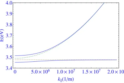
Figure 1.5 | Dispersion of exciton-polaritons in microcavity with GaN QW at zero detuning and

ΩR= 30meV .

Figure 1.5 shows theoretically calculated polariton dispersion for a GaN based microcavity. In vicinity of k_∥ = 0 we can use eﬀective mass approximation to obtain the polariton mass

m+,− =~2(

∂2_E

+,−(k∥)

∂k_∥2 )

−1_. _(1.60)

At resonance m+= m− ≃ 2mph, which is extremely small: about ﬁve orders of magnitude

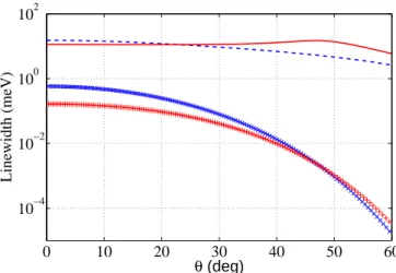
smaller than the exciton mass. An important consequence of this ultra small mass is that polaritons eﬃciently average out the random potential, thus having smaller line-widths [17] than bare excitons and photons.

1.3.3 Polariton-polariton interaction in microcavities

It has been pointed out that polaritons are quasi-particles formed by photons and excitons which are itself composite particles. Experimentally it is known that excitons show bosonic behavior up to high densities [18], though there are some theoretical works [19] putting in question the treatment of excitons like bosons. Nevertheless, based on the ﬁrst heuristical argument there exists an agreement that (at least at not very high densities) they can be considered like pure bosons obeying usual bosonic commutation relation

[ˆbk, ˆb†_k′] = δ_k,k′ (1.61)

(we condense the subscript || in k to shorten the notation). Polariton-polariton interac-tions is due to the mutual interaction of excitons. Neglecting the spin degree of freedom it is

ˆ

(26)

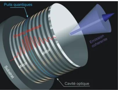
Figure 1.6 | A sketch of a typical microcavity (from private communication with Dr. Dmitry

Sol-nyshkov). An semiconductor QW is embedded between the Bragg mirrors in the anti-nodes of the cavity ﬁeld providing an eﬃcient overlap of exciton and photon

where ˆ Hexc−exc = ∑ k,k′,q vexc−exc(k, k ′ , q)ˆb†_k+qˆb† k′−q ˆ b_k′ˆbk, (1.63)

is the term including exciton-exciton scattering due Coulomb interaction and Pauli ex-clusion principle in which two excitons exchange momentum ~q and

ˆ Hsat = ∑ k,k′,q vsat(k, k ′ , q)ˆa†_k+qˆb† k′−q ˆ b_k′ˆb_k, (1.64)

is the saturation term coming only from Pauli exclusion. It is a process in which the scattering of two excitons of momenta~k, ~k′ produce a photon with momentum~(k + q) and an exciton of momentum~(k′− q). The ﬁrst term 1.63 is always positive referring to

repulsive interaction between excitons of the same spin. Interaction of opposite spins is an open question [20, 21] although, it is usually considered to be much smaller than those of the same spins.

Contrary to this, the sign of interaction of the excitons with the photon ﬁeld in Hsat is

always negative. The exact calculation of matrix elements vexc−exc and vsat determining

the magnitudes of two interactions is a cumbersome task and not entering in details we will use the result obtained in [22, 23]. The matrix elements vexc−exc(k, k

′

, q) and vsat(k, k ′

, q)

in zero-momentum limit read

vexc−exc = 3Eb(a2DB )2 S , (1.65) vsat =−~Ω R nsatS , (1.66)

(27)

where S is the quantization surface and nsat is the so-called saturation density. In

mean-ﬁeld approximation ˆb†_kˆb′_k ∼ δk,k′nexck , where nexck is the exciton density in the state k thus

giving for ˆHsat

ˆ Hsat ∼ − ∑ k nexc nsat_S~ΩR(ˆa † kˆbk+ h.c.), (1.67)

which in fact reduces linear exciton coupling ~ΩR, since exactly at nexc = nsat

exciton-photon coupling vanishes (nsat ∼ (a2DB )−2).

Starting from the interaction written on the exciton-photon basis one may obtain an eﬀective polariton-polariton interaction Hamiltonian. This prescription is obtained as previously by linear Hopﬁeld transformation. Restricting ourselves to only the lower polariton branch, as population of upper polaritons is in most of situations very small, polariton-polariton interaction in the new basis takes the form

ˆ H_int+ = 1 2 ∑ k,k′,q V (k, k′, q)ˆp†_k+qpˆ_k′−q† pˆk′pˆk. (1.68)

where the eﬀective interaction term now includes both contributions. The matrix element is

V (k, k′, q) = vexc−excX_k+q− X_k′−_−qX_k−X_k′−+ vsatX_k′−_−q(C_k+q− X_k−+ X_k+q− C_k−)X_k+. (1.69)

with X_k− and C_k− being the exciton and photon fraction deﬁned by expressions 1.57 and 1.57. In what follows we will neglect saturation term assuming that n+_sat >> nexc,+_{. Then}

all polariton-polariton interactions come from the interaction of excitons with excitons. It is why in polariton basis the matrix element for this interaction in exciton-photon basis is multiplied by Hopﬁeld’s coeﬃcient X_k+ which describes the excitonic contribution to polariton state.

1.4 Bose-Einstein condensation

1.4.1 Bose-Einstein condensation of ideal Bose gas

Indistinguishability of quantum mechanical particles reﬂects the properties of many-particle wave function under permutation symmetry. Interchanging two coordinates in wave function ψ(r1, ..., rN) should give the same physical state which diﬀers from the

initial one only to a phase factor α [24]

ψ(r1, ..., rj, ..., rk, ..., rN) = αψ(r1, ..., rk, ..., rj, ..., rN) = α2ψ(r1, ..., rj, ..., rk, ..., rN).

(1.70) It is obvious that α = ±1. The particles which wave function transforms symmetrically under interchange of coordinates are called bosons (α = 1) whereas anti-symmetric wave

(28)

BOSE-EINSTEIN CONDENSATION 27

function describes fermions (α =−1):

ψ(r1, ..., rj, ..., rk, ..., rN) = +ψ(r1, ..., rk, ..., rj, ..., rN)(bosons), (1.71)

ψ(r1, ..., rj, ..., rk, ..., rN) = −ψ(r1, ..., rk, ..., rj, ..., rN)(f ermions). (1.72)

For given temperature T bosons obey Bose-Einstein and fermions Fermi-Dirac statistics [25].We write both in the short notation

ni(T ) =

1

exp β(ϵi− µ) ∓ 1

(1.73) where ni denotes the most probable occupation number in thermodynamic limit (V →

∞,N → ∞).The factor β = 1/kT and −(+) stands for bosons (fermions). ϵi are the

eigen-values of single-particle Hamiltonians and the chemical potential is deﬁned by nor-malization

N =∑

i

ni(µ, T ) (1.74)

fixing the total number of particles N . Satyendra Nath Bose was the first to propose what is now called Bose-Einstein statistics which Einstein used as a photon statistic to explain the Planck distribution. This preceded the famous paper [26] of Einstein on the subject of this section but also the Fermi statistics. Fermions and bosons show quite different properties. For fermions holds the Pauli principle which forbids two identical fermions to occupy the same state. It is clearly seen putting rj = rk in equation 1.72. Contrary to

fermions, it turns out that bosons have the tendency to ﬁll the same quantum state by condensing in the Bose-Einstein sense.

To see this let’s consider non-interacting bosons with dispersion ϵk = ~2k2/2m and

change summation over i in 1.74 by k

N =∑

k

1

exp β(ϵk− µ) − 1

. (1.75)

Substituting x = k/(√2m/β~2_{) and taking thermodynamic limit we get expression}

nλ3 = g3/2(z), (1.76)

where λ = ~/√2πmkT is thermal de Broglie wavelength and z = exp(βµ) is fugacity. The RHS is integral representation of Bose function

gk(z) = ∞

∑

l=1

zl/lk. (1.77)

The series 1.77 converge for z ≤ 1 and is bounded by value g3/2(z = 1)

g3/2(1) =

∞

∑

l=1

(29)

0.0 0.2 0.4 0.6 0.8 1.0 1.2 0.0 0.2 0.4 0.6 0.8 1.0 1.2 TTC N0 N

Figure 1.7| Condensate fraction showing that at T = TC particles undergo transition to the from Bose

gas to BEC condensate state with k = 0

The last denotes famous Riemann zeta function ζ(z). Equation 1.76 has a solution if

nλ3 ≤ ζ(3/2). (1.79)

Once the condition is fulﬁlled nλ3 = ζ(3/2) we can easily imagine a situation when we either increase n or decrease T and by doing this violate the last inequality. This, in fact, does not happen as the expression 1.76 is obtained in thermodynamic limit replacing

1 V ∑ k → ∫ d3_k (2π)3 (1.80)

in which the term for k = 0 vanishes. Removing thermodynamic limit the expression for large but ﬁnite volume V reads

N V = 1 V z 1− z + ∫ k d3_k (2π)3 1 z−1exp (β~2k2 2m )− 1 , (1.81)

where the first term corresponds to k = 0 and the second one for the states with k ̸= 0. Instead, violating the condition 1.79, particles prefer to condense into k = 0 state which thus becomes macroscopically occupied. This is what is called Bose-Einstein condensation. During the process of condensate forming z stays fixed at z = 1 and in the limit V → ∞ the first term of 1.81, being the condensate density n(k = 0) is indeterminate, otherwise for z ̸= 1 it is zero. This critical point defines the temperature TC of BEC at a given

density n or vice versa:

kTC = 2π~2 m ( n ζ(3/2)) 2/3 , (1.82) nC = ζ(3/2)( mkT 2π~2) 2/3_. _(1.83)

(30)

Figure 1.8 | Distribution of particles in the momentum space. Temperatures are 400 nK, 200 nK, and

50nK (from left to right)[5]. Macroscopical occupation occurs for T < TC(central and right distributions)

Using the deﬁnition of critical temperature and relation 1.76 we ﬁnd the fraction of par-ticles being in Bose-Einstein condensate:

N0

N = (1− ( T TC

)3/2). (1.84)

The condensate fraction is zero below TC. Lowering the temperature, thermal part 1−

N0/N decreases and at T = 0K all particles are forced to condense (the Fig. 1.7). For

the ﬁrst time BEC was observed by E. Cornell,C. Wieman et al. [5] seventy years after Einstein’s paper [26]. The experiment consist in cooling rubidium-87 atoms below the critical temperature TC = 170nK. The Figure 1.8 shows the distribution of particles at

three diﬀerent temperatures of this experiment. It’s clearly seen that at the temperatures far below the critical one, most of the particles occupy the ground state k = 0.

1.4.2 Bose-Einstain condensation in weakly-interacting gases

The previous section was dedicated to BEC in an ideal Bose gas in three dimensions. As we have seen, cavity polaritons are 2D objects. It is interesting to see how BEC depends on the dimensionality of the system in the question. Coming back to expression 1.81, one can easily check that the thermal part which we denote like

nT = ∫ k d3_k (2π)3 1 z−1exp (β~_2m2k2)− 1, (1.85) shows infrared divergence in 1D and 2D, and converges to some deﬁnite value nc_T for 3D in the limit z = 1, which we is said to be the fugacity value during occurrence of BEC phase transition. In this manner in three spatial dimensions all particles N − N_Tc

(31)

at ﬁnite temperatures T < TC are obliged to descent into condensate, as the capability

to accommodate new particles in the thermal part is exhausted by reaching nc_T. This is not true for 1D and 2D situations - the integral 1.85 is inﬁnite due to contributions at

⃗k ≈ 0 and the condensation at ﬁnite temperature can’t take place. Adding new particles

we will increase the density of thermal part but not that of the condensate as in this case

nT is an unbounded function. For one-dimensional Bose gas this holds also at T = 0.

This is the consequence of one ”no-go” theorem [27] under name of Mermin, Wagner, and Hohenberg. It forbids that a continuous symmetry could be spontaneously broken in dimensions less then three. The spontaneous symmetry breaking means that there is some physical observable which was zero before BEC transition and which takes a non-zero value in the condensed phase. This observable is called the order parameter. BEC is a second order phase transition in which at T = TC U (1) symmetry,representing the phase

freedom of normal Bose gas and being continuous, spontaneously disappears at T = Tc.

BEC formed in this transition ﬁxes its phase to some particular value and following mentioned theorem it is not in principle possible in 1D and 2D. But this restriction refers exclusively to the spontaneous symmetry breaking of a continuous symmetry and not to phase transitions in general.

It is well known that in 2D systems another kind of thermodynamical phase transition occurs - Berezinskii-Kosterlitz-Thouless (BKT) phase transition [28] to a superﬂuid phase. ’Spontaneous’ binding of thermally excited vortices of opposite directions establishes at some temperatures T = TBKT, while a free vortex could be observed at T > TBKT. BKT

phase transition is not a second order phase transition - there is not an order parameter vanishing as soon as the last condition is fulﬁlled. Instead of disappearance of the order parameter the change is more qualitative and one can speak about ”quasi-condensate”.

In finite systems 1D and 2D, the convergence of the expression 1.85 is recovered. But in a finite system z cannot reach one. This means that the particle number in condensate is not macroscopically but rather significantly larger than the particle number in thermal part.

If we want to consider BEC of polaritons as we have seen before, we have to include polariton-polariton interaction. To do this we introduce one-body density matrix

n(⃗r, ⃗r′) =< ˆψ†(⃗r) ˆψ(⃗r′) >, (1.86) where ˆψ†(⃗r), ˆψ(⃗r′) are creation and annihilation operators of our Bose ﬁeld satisfying

ˆ

ψ(⃗r) = ϕ0(⃗r)ˆa0(⃗r) +

∑

i

ϕi(⃗r)ˆai(⃗r). (1.87)

The ﬁeld operator is expanded over single particle states deﬁned in general case by eigen-problem of density matrix 1.86

∫

(32)

The density matrix describes correlations of Bose ﬁeld in two space points ⃗r and ⃗r′. Equation 1.87 allows us to write the density matrix in the form

n(⃗r, ⃗r′) = n0(⃗r, ⃗r ′ ) + ˜n(⃗r, ⃗r′) = N0ϕ∗0(⃗r)ϕ0(⃗r′) + ∑ i̸=0 Niϕ∗i(⃗r)ϕi(⃗r′). (1.89)

The ﬁrst term represents occupation of BEC and the second one occupation of thermal reservoir. The density matrix of the latter decays exponentially with distance s =|r′− r| with characteristic length λT =

√

2π~/mkBT . Correlations are present only on this

scale whereas for s > λT thermal part of the system is uncorrelated, independent of

the temperature. However, the density-matrix n0(⃗r, ⃗r

′

) below the critical temperature

T < TC shows ﬁnite correlations in the limit s→ ∞ contributing to the ﬁnite correlations

of total density matrix. This should be supported, as its Fourier transform is equal to

⃗k-distribution n(⃗k), by particle distribution below T < TC of the form

N (⃗k) = N0δ(⃗k) + ˜N (⃗k). (1.90)

The above distribution recovers the condition of the macroscopical occupation of the ground state for finite systems. Finite correlations in the long-range limit (s → ∞) or off-diagonal long-range is called Penrose-Osanger criterion of BEC [28] which is a well-defined criterion not only in an ideal Bose gas, but also in a weakly interacting nonuniform system. In what follows we will assume that interaction between particles can be characterized by s-wave scattering length a which enables witting the condition of diluteness in the form: a << n1/3 _{and apply Bogoliubov approach. The approximation}

consists of replacing the creation and annihilation operators, ˆa0 and ˆa†0, in Hamiltonian

of weakly-interacting bosons ˆ H =∑ k E_⃗_k0ˆa_⃗† kˆa⃗k′ + g 2V ∑ ⃗ k,⃗k′,⃗q ˆ a†_⃗ k+⃗qˆa † ⃗ k′−⃗qˆa⃗kˆa⃗k′. (1.91) by complex numbers ˆ a0, ˆa†0 → √ N0. (1.92)

which is applicable always when the density of ground state remains ﬁnite and depletion is not very strong N − N0 << N , in thermodynamic limit. The interaction constant

g ≈ 4π~2a/m. For ﬁxed number of particles number operator ˆN

ˆ N =∑ ⃗_k ˆ a†_⃗ kˆa⃗k ≈ N0+ 1 2 ∑ ⃗ k̸=0 (ˆa_⃗† kˆa⃗k+ ˆa † −⃗kˆa−⃗k). (1.93)

can be replaced by its eigenvalue N . After some straightforward calculation, which in-cludes keeping the terms of order N and N2 only, one obtains:

ˆ H≈ gN 2 2V + 1 2 ∑ ⃗ k̸=0 (E⃗_k0 + ng)(â_⃗† kaˆ⃗k+ â † −⃗kˆa−⃗k) + ng(â † ⃗ kâ † −⃗k + ˆa⃗kaˆ−⃗k). (1.94)

(33)

which is reasonable as has been pointed out in the case of small depletion. Introducing Bogoliubov transformation of operators

ˆ a⃗_k = u⃗_kαˆ_k⃗ − v⃗_kαˆ†_−⃗k, (1.95) ˆ a† −⃗k = u⃗kαˆ † −⃗k − v⃗kαˆ⃗k, (1.96)

where coeﬃcients u⃗_k and v⃗_k satisﬁes

v_⃗_k2 = u_⃗2_k− 1 = 1 2( E_⃗0 k+ ng E⃗_k − 1) (1.97) the Hamiltonian 1.94 in terms of new quasi-particle operators reads

ˆ H = 1 2gn 2_V ₋ 1 2 ∑ ⃗_k_̸=0 (E_⃗_k0+ ng− E⃗_k) + 1 2 ∑ ⃗ k̸=0 E⃗_k( ˆα⃗_k†αˆ⃗_k+ ˆα†_−⃗kαˆ_−⃗k), (1.98) where E⃗_k = √ (E0 ⃗ k) 2_{+ 2ngE}0 ⃗ k. (1.99)

It is the famous Bogoliubov dispersion law of elementary excitations of the system as it refers to states with ⃗k ̸= 0. The obtained Hamiltonian makes possible to describe the excited states of an interacting Bose gas like the ones of the non-interacting gas of Bogoliubov quanta. The dispersion law in long-wavelength and short-wavelength limit is

E⃗_k = { c⃗k (⃗k → 0) E0 ⃗_k+ gn (⃗k → ∞) (1.100)

The former corresponds to sound waves - phonons with velocity c =√gn/m and the latter

gives the dispersion of free particles. Transition from phonon to free particle dispersion occurs when E_⃗0

k ≈ gn deﬁning healing length

ξ = √ 1

8πna. (1.101)

1.4.3 Bose-Einstain condensation in non-uniform systems

The ﬁrst observation of the BEC phase transition of Cornell group 1.8 was done for a trapped atoms - an non-uniform system. As in practice this is rather a rule than exception, this section will be dedicated to BEC in non-uniform gases. In the spirit of Bogoliubov approximation we replace the ﬁeld operator of the spatial coordinate ⃗r in time instant t

with a classical ﬁeld

ˆ

ψ(⃗r) = ψ0(⃗r) + δ ˆψ(⃗r). (1.102)

In mean-ﬁeld approximation ψ0(⃗r) =< ˆψ(⃗r) > and as < δ ˆψ(⃗r) >= 0 we will neglect

(34)

parameter. For a weakly interacting dilute Bose gas in some external potential Vext(⃗r)

from Hamiltonian 1.91 given in ⃗k-space we can write second quantization Hamiltonian in real space ˆ H = ∫ d3⃗r( ~ 2 2m∇ ˆψ †_{∇ ˆ}_{ψ + ˆ}_ψ†_V ext(⃗r) ˆψ) + ∫ ∫ d3⃗rd3⃗r′( ˆψ†ψˆ′†V (⃗r− ⃗r′) ˆψ ˆψ′) (1.103) As interaction is constant in ⃗k-representation: g = 4π~/m in r-representation it will have contact interaction V (r− r′) = gδ(r− r′) which assumes scattering of hard spheres of the radius a. From the previous Hamiltonian we write an energy functional as follows

E = ∫ d3⃗r( ~ 2 2m|∇ψ0| 2 _{+ V} ext(⃗r)|ψ0|2+ g 2|ψ0| 4_), _(1.104)

bearing in mind that we neglected ’ﬂuctuations’ by performing the mean-ﬁeld approxi-mation. Variational procedure with the above energy functional gives an equation for the order parameter i~∂ ∂tψ0(⃗r, t) = ( ~2∇2 2m + Vext(⃗r) + g|ψ0(⃗r, t)| 2_)ψ 0(⃗r, t). (1.105)

The obtained equation is the famous Gross-Pitaevskii (GP), a non-linear Schr¨ odinger-type equation, with an exception that it is its quantum version (contains ~) describing one nonclassical quantity - the probability amplitude ψ0(⃗r, t). As ψ0(⃗r, t) is no more

operator but rather a complex number in each ⃗r and t one has:

ψ0 =|ψ0|exp(iχ); N0 =|ψ0|2; ⃗v =

~

m∇χ. (1.106)

The last two expressions describe number of particles in BEC (in a dilute system N0 ≈ N)

and velocity.

The time-dependence of the ground state is given by: ψ0(⃗r, t) = ψ0(⃗r)exp(−iµt), where

µ is the chemical potential and GP equation becomes:

(~

2_∇2

2m + Vext(⃗r)− µ + g|ψ0(⃗r)|

2_)ψ

0(⃗r) = 0 (1.107)

Immamoglu and Ram [6] were ﬁrst to theoretically consider a polariton BEC in frame of one novel type of laser: polariton laser. Besides the conceptual importance of BEC in a solid state system very small polariton mass opens a way to study BEC at higher temperatures, as the temperature of phase transition TC is inversely proportional

to mass of particles (see expression1.82). The ﬁrst experimental observation of BEC for microcavity polaritons was reported in 2006 [29]. Room-temperature polariton laser has been proposed in 2002 by Malpuech et al. [7].

An important characteristic of polaritons it is their ﬁnite-life time. Polaritons in lower dispersion branch in the ⃗k_∥ = 0 state have the life time much shorter than in excited

(35)

(a)

(b)

Figure 1.9 | Bose-Einstein condensation of microcavity polaritons [29]: (a) Emission pattern vs

excita-tion powers at 5K (form the left to the right). (b) Energy resolved spectra of panel (a)

state, as the life-time is proportional to photon fraction which we have seen to decrease with ⃗k_∥ . Then, if polariton population is is created somewhere on the lower polariton branch ⃗k_∥ ̸= 0, one should have eﬃcient relaxation mechanisms in order to thermalize and reach a macroscopical occupation of ground state forming BEC. More details on this interesting question concerning quantum kinetics and thermodynamics of polaritons can be found in ref. [30].

1.5 Pseudo-spin of exciton-polaritons

In section 1.1 on excitons and quantum conﬁnement, we have seen that a heavy exciton is composed of an electron having a one half spin and a heavy hole state which due orbital angular momentum L = 1 makes total angular momentum J = 3/2. The operator of total angular momentum along quantization axis (growth axis)for excitons is thus given by

ˆ

J_zexc= (sh_z + l_zh)ˆσz⊗ ˆI+ ˆI⊗ sezσˆz. (1.108)

ˆ

I is 2×2 unity matrix and ˆσz z-Pauli matrix. For jzh = jzhh = shhz + lzhh= 3/2 and sez = 1/2

the z-component of total angular momentum operator for a heavy hole exciton is

ˆ J_zexc=      2 0 0 0 0 −1 0 0 0 0 1 0 0 0 0 −2     . (1.109)

Exciton-polaritons dans les systèmes de dimensionnalité basse

HAL Id: tel-00632151

https://tel.archives-ouvertes.fr/tel-00632151

To cite this version:

UNIVERSITE BLAISE PASCAL

THESE

Goran PAVLOVIC

Exciton-Polaritons in Low-Dimensional

Structures

WHITTAKER David

rapporteur

KAVOKIN Alexey

rapporteur

RICHARD Maxime

examinateur

SHELYKH Ivan

Pr`

esident

MALPUECH Guillaume

directeur de Th`

ese

GIPPIUS Nikolay

directeur de Th`

ese

Contents

Acknowledgment

Introduction

Chapter 1