Autonomous Thruster Failure Recovery for
Underactuated Spacecraft
by
Christopher Masaru Pong
B.S.,
Harvey Mudd College (2008)
MASSACHUSEN S INSTITUTE
OCT 18 2
L_RI-kRES
Submitted to the Department of Aeronautics and Astronautics
in partial fulfillment of the requirements for the degree of
Master of Science in Aeronautics and Astronautics
at the
MASSACHUSETTS INSTITUTE OF TECHNOLOGY
ARCHIVES
September 2010
@
Massachusetts Institute of Technology 2010. All rights reserved.
Author ...
....
...
Department of Aeronautics and Astronautics
7/
August 19, 2010
Certified by...
David W. Miller
Professor of Aeronautics and Astronautics
A i A
Thesis Supervisor
Certified by...
Alvar Saenz-Otero
Research Scientist, Aeronautics and Astronautics
I
. Thesis Supervisor
Accepted by ...
Associate Professor f
Eytan H. Modiano
Aeronautics and Astronautics
Chair, Graduate Program Committee
Autonomous Thruster Failure Recovery for Underactuated
Spacecraft
by
Christopher Masaru Pong
Submitted to the Department of Aeronautics and Astronautics on August 19, 2010, in partial fulfillment of the
requirements for the degree of
Master of Science in Aeronautics and Astronautics
Abstract
Thruster failures historically account for a large percentage of failures that have oc-curred on orbit. Therefore, autonomous thruster failure detection, isolation, and recovery (FDIR) is an essential component to any robust space-based system. This thesis focuses specifically on developing thruster failure recovery techniques as there exist many proven thruster FDI algorithms. Typically, thruster failures are handled through redundancy-if a thruster fails, control can be allocated to other operational thrusters. However, with the increasing push to using smaller, less expensive satellites there is a need to perform thruster failure recovery without additional hardware, which would add extra mass, volume, and complexity to the spacecraft. This means that a thruster failure may cause the spacecraft to become underactuated, requiring more advanced control techniques. Therefore, the objective of this thesis is to develop and analyze thruster failure recovery techniques for the attitude and translational control of underactuated spacecraft.
To achieve this objective, first, a model of a thruster-controlled spacecraft is de-veloped and analyzed with linear and nonlinear controllability tests. This highlights the challenges involved with developing a control system that is able to reconfig-ure itself to handle thruster failreconfig-ures. Several control techniques are then identified as potential candidates for solving this control problem. Solutions to many issues with implementing one of the most promising techniques, Model Predictive Control (MPC), are described such as a method to compensate for the large delays caused
by solving an nonlinear programming problem in real time. These control techniques
were implemented and tested in simulation as well as in hardware on the SPHERES testbed. These results show that MPC provided superior performance over a sim-ple path planning technique in terms of maneuver comsim-pletion time and number of thruster failure cases handled at the cost of a larger computational load and slightly increased fuel usage. Finally, potential extensions to this work as well as alternative methods of providing thruster failure recovery are provided.
Thesis Supervisor: David W. Miller
Title: Professor of Aeronautics and Astronautics Thesis Supervisor: Alvar Saenz-Otero
Acknowledgments
There are many people that I would like to thank who have made the completion of this thesis possible. To Professor David W. Miller and Dr. Alvar Saenz-Otero who provided guidance, kept me motivated, and allowed me the freedom to work on intriguing problems. To the SPHERES team, Jake Katz, Jaime Ramirez, Chris Mandy, Jack Field, Enrico Stoll, Martin Azkarate, Brent Tweddle, Swati Mohan, Caley Burke, Amer Fejzid, Carlos Andrade, Steffen Jdekel, and David Pascual for their mentorship, advice, and overall assistance in making SPHERES experiments at MIT and especially on the ISS a possibility. To my officemates, Matt Smith and Zach Bailey, for their friendship and willingness to help. To my classmate, Andy Whitten, who always provided much-needed comic relief. To my mom, dad, brother and soon-to-be family-in-law who I can always count on for support. Finally, to my fiancee, Julia Kramer, who graciously followed me across the country so that I could pursue my dreams.
Contents
1 Introduction
1.1 M otivation . . . . 1.2 Overview of the SPHERES Testbed . . . .
1.3 Approach & Thesis Overview . . . .
2 Literature Review & Gap Analysis
2.1 Thruster Fault Detection and Isolation . . . . 2.2 Thruster Failure Recovery . . . .
2.3 G ap A nalysis . . . .
3 Spacecraft Model
3.1 Rigid-Body Dynamics . . . .
3.1.1 Reference Frames & Rotations . . . .
3.1.2 Attitude Kinematics & Kinetics. . . . .. 3.1.3 Translational Kinematics & Kinetics. . . . .. 3.2 Equations of Motion of a Thruster-Controlled Spacecraft
3.2.1 Six-Degree-of-Freedom Model. . . . . . . . ..
3.2.2 Three-Degree-of-Freedom Model . . . .
3.3 Controllability . . . . 3.3.1 Linear Time-Invariant Controllability . . . .
3.3.2 Small-Time Local Controllability . . . . 3.4 Sum m ary . . . . 15 15 19 21 23 23 27 29 31 . . . . 31 . . . . 32 . . . . 35 . . . . 37 . . . . 37 . . . . 38 . . . . 39 . . . . 40 . . . . 41 . . . . 45 . . . . 54
4 Thruster Failure Recovery Techniques 57
4.1 Control System Design Challenges . . . . 57
4.1.1 Coupling.. . . . . . . 58
4.1.2 Multiplicative Nonlinearities . . . . 59
4.1.3 Saturation . . . . 60
4.1.4 Nonholonomicity . . . . 61
4.2 Reconfigurable Control Allocation . . . . 61
4.2.1 Redistributed Pseudoinverse . . . . 66
4.2.2 Active Set Method . . . . 68
4.3 Path Planning . . . . 69
4.3.1 Piecewise Trajectory . . . . 69
4.3.2 Rapidly Exploring Dense Trees . . . . 70
4.4 Model Predictive Control . . . . 73
4.4.1 Stability . . . . 76
4.4.2 Optimality . . . . 78
4.5 Sum m ary . . . . 79
5 Model Predictive Control Implementation Issues 81 5.1 Regulation & Attitude Error.. . . . . . . . 81
5.2 Nonlinear Programming Algorithm .. . . . .. 83
5.2.1 Selection.. . . . . . . . . 83
5.2.2 Implementation... . . . . . . . . . . . 85
5.3 Processing Delay... . . . . . . . . . 87
5.4 Feasibility & Guaranteed Stability . . . . 89
5.5 Sum m ary . . . . 91
6 Simulation & Hardware Testing Results 93 6.1 Six-Degree-of-Freedom Results . . . . 93
6.1.1 Baseline Translation . . . . 95
6.1.2 Reconfigurable Control Allocation . . . . 96
6.1.4 Model Predictive Control . . . . 103
6.2 Three-Degree-of-Freedom Results . . . . 107
6.2.1 Baseline Translation . . . . 108
6.2.2 Model Predictive Control . . . . .. 108
7 Conclusion 113 7.1 Thesis Sum m ary . . . . 113
7.2 Contributions . . . . 117
7.3 Recommendations & Future Work . . . . 119
A Small-Time Local Controllability of SPHERES 121 A.1 Three-Degree-of-Freedom SPHERES Model . . . . 122
A.2 Six-Degree-of-Freedom SPHERES Model . . . . 125
B Optimization 129 B.1 Nonlinear Programming: Sequential Quadratic Programming . . . . . 129
B.2 Quadratic Programming: Active Set Method . . . . 140
List of Figures
1-1 Distribution of attitude and orbit control system failures. . . . . 16
1-2 Artist's conception of DARPA's System F6. . . . . 18
1-3 SPHERES satellites on the ISS. . . . . 19
1-4 SPHERES satellite without shell. . . . . 19
2-1 NASA's Cassini spacecraft with direct redundancy. . . . . 28
2-2 ESA's Automated Transfer Vehicle with functional redundancy. . . . 28
3-1 Thruster locations, directions and physical properties for an example 3DOF spacecraft. . . . . 44
3-2 Pictorial representation of flow along vector fields producing non-zero net m otion. . . . . 46
3-3 Differential-drive example showing a series of four motion primitives. 47 3-4 Thruster locations and directions for 3DOF SPHERES spacecraft. . . 52
3-5 Thruster locations and directions for 6DOF SPHERES spacecraft. . . 53
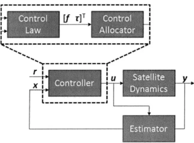
4-1 Decomposition of a controller into a control law and control allocator. 62 5-1 Example showing how the SQP algorithm iteratively approaches the constrained global optimum of the Rosenbrock function. . . . . 86
5-2 Delay compensation method for mitigating the effects of processing delay. 88 6-1 Thruster locations and directions for 6DOF SPHERES spacecraft. . . 94
6-2 6DOF representative maneuver: PD control, all thrusters operational (simulation)... ... ... . . . . . . ... 96
6-3 6DOF representative maneuver: PD control, thruster 9 failed
(simula-tion ). . . . . 9 7
6-4 6DOF representative maneuver: PD control with redistributed weighted pseudoinverse, thruster 9 failed (simulation). . . . . 98 6-5 6DOF representative maneuver: PD control with active set method,
thruster 9 failed (simulation). . . . . 99 6-6 6DOF representative maneuver in the opposite direction: PD control
with active set method, thruster 9 failed (simulation). . . . . 100 6-7 6DOF representative maneuver in opposite direction: PD control with
active set method, 0.95 weight on torque, 0.05 weight on force, thruster
9 failed (sim ulation). . . . 101 6-8 6DOF representative maneuver: PD control, piecewise trajectory
(hard-w are). . . . 102
6-9 Thruster firings for piecewise trajectory test (hardware). . . . 103 6-10 6DOF representative maneuver: MPC, thruster 9 failed (simulation). 106 6-11 3DOF representative maneuver: PD control, all thrusters operational
(hardw are). . . . 109
6-12 3DOF representative maneuver: PD control, thruster 9 failed (hardware).110 6-13 3DOF representative maneuver: MPC, thruster 9 failed (hardware). . 111
A-1 Thruster locations and directions for 3DOF SPHERES spacecraft. . . 122
List of Tables
Variable definitions for the 6DOF model. . . . . Variable definitions for the 3DOF model. . . . . Small-time local controllability of SPHERES. . . . . 5.1 Comparison of the SQP algorithm versus fmincon run time exam ple problem . . . .
6DOF SPHERES parameters. . . . . 6DOF MPC parameters. . . . .
Comparison of the piecewise trajectory and MPC techniques. .
3DOF SPHERES parameters. . . . .
3DOF MPC parameters... . . . . . . .. on an . . . . 94 . . . . 105 . . . . 106 . . . . 108 . . . . 110 3.1 3.2 3.3 6.1 6.2 6.3 6.4 6.5
Chapter 1
Introduction
1.1
Motivation
Failure Detection, Isolation, and Recovery (FDIR) is an integral part of any robust space-based system. If a satellite fails on orbit, currently there is little to no chance of being able to send an agent to that satellite and provide on-orbit servicing. Thus, it is paramount for a satellite to be able to tell if something is wrong (failure detection), determine what subsystem or component has failed (isolation), and appropriately change the system to handle this failure (recovery).
There are many types of spacecraft failures that can occur on orbit. Since it is impractical to create a spacecraft that can autonomously detect, isolate, and recover from all possible failures, it is important to prioritize these these failures to ensure that the most likely failures with a large impact on the mission are handled. To begin, broad classifications of failures will be considered. Sarsfield has classified spacecraft failures into four distinct categories [1]:
* Failures Caused by the Space Environment: This includes space debris
impact, degradation due to atomic oxygen, thermal fluctuations from solar and albedo radiation, charging and arcing due to solar wind, and single-event upsets, latchups, and burnouts from radiation.
sys-tems such as buckling due to incorrect modeling and analysis of the spacecraft structure.
" Failures Related to Parts and Quality: This includes all component failures
not attributed to the environment or design error. These failures normally occur randomly due to degradation over time such as the fatigue of structural components.
" Other Types of Failures: This includes all other types of failures such as
bad commands from ground operators, errors in software, and out-of-bound conditions such as exposure of sensitive optics to direct sunlight.
While all of these types of failures are worthy of further research, this thesis will focus on random component failures, specifically thruster failures. Tafazoli has conducted an extensive review of failures that have occured on 129 military and commercial spacecraft from 1980 to 2005 [2]. One of the many useful results of this study was determining the distribution of failures that have occurred on these spacecraft. Figure
1-1 shows that thruster failures account for 24% of all the Attitude and Orbit Control
System (AOCS) failures.1
U4%CMG * 2% Electronic circuitry w 6% Environment N 8% Fuel tank * 17% Gyroscope 7 2% Oxidizer tank i 16% Reaction wheel * 4% Software error E 24% Thruster a 18% Unknown
Figure 1-1: Distribution of attitude and orbit control system failures [2].
Because thruster failures are one of the more likely failures to occur on a spacecraft, many have developed ways to mitigate the effect of these failures. One of the obvious methods of handling these failures is through the use of additional hardware. Sensors can be embedded in the thruster itself for thruster failure detection (see, e.g., [3]) and additional redundant thrusters can be used to replace the failed thrusters.
Sarsfield provides an interesting view on redundancy [1]: "Historically, redundancy has been a central method of achieving resistance to failure and has been incorpo-rated up to the point at which the incremental costs of including it began to exceed reductions in the cost of failure." In addition to the impact of redundancy on the cost budget, it also impacts mass, volume, and power budgets on the spacecraft.
For large, monolithic spacecraft with a cost budget on the order of billions of dollars, redundancy may well be justified. However, there is a move toward launching smaller, less expensive spacecraft. One example is a payload adapter for the Evolved Expendable Launch Vehicle (EELV) family termed the EELV Secondary Payload Adapter (ESPA) ring [4]. The ESPA ring allows up to six secondary and one primary payload to share a ride to space. By sharing this cost, launching a 180-kg spacecraft on an ESPA ring can be less than 5% of the cost of a dedicated launch vehicle. Another, more extreme, example of less expensive spacecraft are satellites that follow the CubeSat standard [5]. By adhering to this standard, these spacecraft can be launched from a Poly-Picosatellite Orbital Deployer (P-POD) [6], which can be bolted to the upper stage of many different types of launch vehicles (e.g., Rokot, Kosmos-3M, M-V, Dnepr, Minotaur, PSLV, Falcon 1). These CubeSats can be launched at a very small fraction of the launch vehicle cost. Recently, the National Aeronautics and Space Administration (NASA) has announced that it will provide subsidized CubeSat launch opportunities, enabling launches at the cost of $30,000 per CubeSat unit [7]. For these less expensive, smaller satellites, it may very well be more costly to include redundancy than risk failure.
There is also a push to replace the functionality of a monolithic spacecraft with multiple spacecraft. One such example is DARPA's System F6 Program, shown in Figure 1-2. The purpose of this program is to demonstrate a fractionated spacecraft
architecture, where each spacecraft has a specialized role in the cluster. As an exam-ple, there might be one spacecraft that performs most of the computations necessary for the mission and another to gather most of the power for the cluster. The main motivation is that fractionated space architectures are flexible in the face of diverse risks such as component failures, obsolescence, funding continuity, and launch failures
[8].
One of many costs associated with buying this flexibility and robustness is that the cluster as a whole has a lot of redundancy. Even though there may be a single specialized "power" spacecraft, each spacecraft must have its own power subsystem. Including redundancy for each spacecraft to handle failures on top of this, may be too costly to justify the benefits. With the prospect of having multiple spacecraft in a cluster or formation, methods of performing thruster FDIR without the use of hardware redundancy has become a vital topic of research.1.2
Overview of the SPHERES Testbed
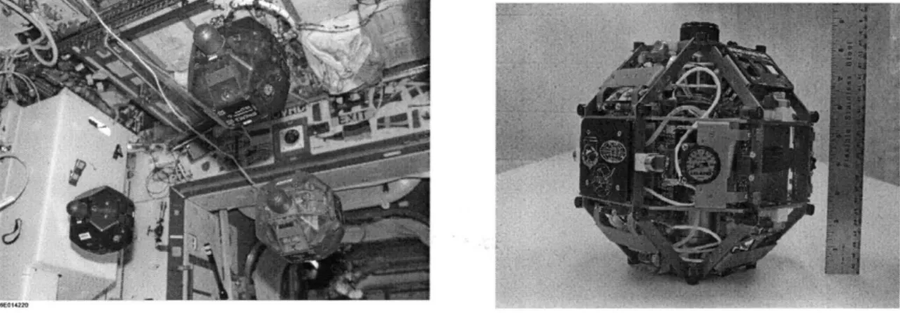
To aid in the development and maturation of estimation and control algorithms for proximity operations such as formation flight, inspection, servicing, assembly, the Massachusetts Institute of Technology (MIT) Space Systems Laboratory (SSL) has developed the Synchronized Position Hold, Engage, Reorient, Experimental Satellites (SPHERES) testbed. This testbed consists of six nanosatellites: three at the MIT
SSL and three on board the International Space Station (ISS). The three satellites on
the ISS can be seen flying in formation in Figure 1-3, and a satellite without its shell can be seen in Figure 1-4. These satellites will serve as a representative spacecraft on which to test the developed thruster FDIR algorithms.
Figure 1-3: SPHERES satellites on the Figure 1-4: SPHERES satellite without
ISS. shell.
The SPHERES satellites contain all the necessary subsystem functionality of a typical satellite:
" Avionics: A Sundance SMT375 is used as the main avionics board, which
includes a processor, memory, and FPGA. A Texas Instruments C6701 DSP performs all the necessary on-board computations for the satellite at a clock speed of 167 MHz. 16 MB of RAM and 512 KB of flash ROM are available as on-board memory. External analog inputs are digitized with a 12-bit D/A on the FPGA.
on two different channels (868 and 916 MHz) at an effective rate of 18 kbps between the satellites and ground station.
" Metrology: Inertial measurements are provided by 3 Q-Flex QA-750
accelerom-eters, and 3 BEI GyroChip II gyroscopes. Measurements of position and atti-tude relative to the surrounding laboratory frame are provided by 24 on-board ultrasound receivers. Time-of-flight data from up to five beacons placed in the laboratory frame to the on-board receivers provide global position to within a few millimeters and attitude to within 1-2 degrees [10].
* Power: 16 AA batteries provide the satellite with an average 15 W at 12 V.
" Propulsion: CO2 is stored in a replenishable tank at 860 psi, fed through a
regulator to be stepped down to 25 psi (set to 35 psi for ground testing), and expelled through 12 solenoid valves and nozzles, each producing around 120 mN of thrust.
Additional information on the SPHERES testbed can be found in [11, 12, 13, 14]. Testing in the space environment is typically a high-risk and costly endeavor where any anomaly or failure can easily result in the loss of a mission (see, e.g., the Demonstration of Autonomous Rendezvous Technology (DART) spacecraft [15]). The SPHERES testbed provides researchers with the ability to push the limits of new algorithms by performing testing in a low-risk, representative environment. If something goes wrong, the astronaut running the SPHERES testbed can simply stop a test and grab the satellites. Three different development environments are used: the six-degree-of-freedom (6DOF) MATLAB simulation, the three-degree-of-freedom
(3DOF) ground testbed, and the 6DOF ISS testbed. These environments allow
algo-rithms to be iteratively matured to higher Technology Readiness Levels, a measure of maturity used by NASA and the Department of Defense (DoD).
1.3
Approach & Thesis Overview
This thesis is divided into seven chapters. Chapter 2 provides a literature review and gap analysis of thruster FDIR and the focuses the thesis on thruster failure recovery techniques. Chapter 3 derives the model of a thruster-controlled spacecraft and analyzes the controllability of the model using linear and nonlinear techniques. Chapter 4 outlines the challenges associated with developing a controller that is able to handle thruster failures, analyzes techniques to handle these challenges, and selects three candidate control techniques. Chapter 5 reveals many of the implementation issues that are not addressed in the theory of Model Predictive Control (MPC), the most promising control technique for thruster failure recovery. Chapter 6 presents the results of simulation and hardware testing of the various thruster failure recovery techniques. Chapter 7 concludes the thesis with contributions and recommendations for future work.
Chapter 2
Literature Review & Gap Analysis
This chapter provides a summary of the literature on thruster FDIR and a discus-sion of the gap in the literature that will be addressed by this thesis. The chapter is organized into three sections. Section 2.1 reviews the methods that have been employed to detect and isolate both general actuator failures as well as methods de-veloped specifically for thruster failures. Section 2.2 discusses how thruster failures are normally handled through control allocation as well as more advanced methods for controlling the attitude of underactuated spacecraft. Finally, Section 2.3 discusses how the literature has not addressed the issue of controlling the attitude and trans-lational dynamics of a spacecraft that has become underactuated due to a thruster failure.
2.1
Thruster Fault Detection and Isolation
One option for detecting thruster failures is through the use of specialized pressure and temperature sensors in the nozzle of a thruster. This, however, comes at the price of extra mass, cost and complexity. This section instead provides a survey of generalizable methods of performing thruster FDI using only additional software and hardware already on board.
Kalman filters inherently have a built-in failure detection scheme: the Kalman filter innovation. This is defined as the difference in the measured output of the
system, and the estimated output of the system. In the nominal case, it is assumed that the plant model approximates the actual system reasonably well. For this nomi-nal operating condition, there will always be some non-zero Kalman filter innovation due to process and sensor noise, from which the baseline threshold can determined. Where this threshold is placed exactly, brings up the underlying trade that must be made for all FDI systems: detection speed versus accuracy. When a failure occurs, the estimated and measured outputs begin to diverge. This happens because the es-timator no longer accurately models the system-the system dynamics have changed due to the failure. When the innovation passes through the set threshold, a failure is detected. Therefore, if the threshold is set too low, false failures may be detected. However, if the threshold is set too high, the time before detection increases.
Willsky [161 has outlined numerous methods of creating failure-specific filters, where the gains of the estimator can be tweaked or the weights of the estimator can be weighted in such a way that it is more sensitive to specific failures. Thus, when one of those failures occurs, the failure is detected and isolated to a smaller subset of possible failures. The innovations can also be analyzed for specific signatures that only a particular failure would have. Because these filters are tweaked from their more optimal configuration, it is common to employ a normal filter for state estimation and have a 'failure-monitor' filter that detects failures. Recently, Chen and Speyer have developed a least-squares filter that explicitly monitors a single failure while ignoring all other failures [17]. This is done by reformulating the least-squares derivation for a Kalman filter, such that one particular failure is highlighted while other similar or 'nuisance' faults are placed in an unobservable subspace.
The next logical step to detect multiple possible failures is to run multiple Kalman filters simultaneously. Work by Willsky, Deyst and Crawford [18] develop the use of a bank of Kalman filters, based off the work of Buxbaum and Haddad [19]. There is a single Kalman filter for every expected failure type as well as the no-failure case. These filters are created with the different dynamics of the various failure modes. Therefore, when the system is operating under nominal conditions, all the Kalman filters would have high innovations except for the nominal filter. When a
failure occurs, the nominal filter innovation increases (indicating a failure) and the innovation of the filter monitoring the failure that occured decreases (isolating the failure). While this is an intuitively simple method of detecting failures, it is extremely computationally intensive since it is running multiple Kalman filters in parallel. One possible way of reducing the computation of this bank of filters is to only run the nominal filter until a failure- is detected. When this occurs, the other filters can be initialized and run until the failure is isolated. When it is isolated, the other filters can be turned off. This trades a longer isolation time with less computational power.
A different FDI technique developed specifically for thruster failures is
maximum-likelihood FDI originally developed for the Shuttle reaction control subsystem jets
by Deyst and Deckert [20]. It is an intuitive method that uses knowledge of the thruster geometry of the spacecraft as well as inertial measurement unit (IMU) data to determine which thruster has failed, if any. From the thruster geometry, one can calculate the expected body-fixed rotational and translational accelerations for each thruster, called influence coefficients. It must be noted here that for thrusters that are placed in relatively close proximity and similar directions, the influence coefficient are near identical. Thruster force variations along with only slightly different thrust directions and moment arms means that it is difficult to distinguish failures between these thrusters without exercising each one individually. These thruster influence coefficient vectors are stored in memory for future use. An estimator for the rotational and translational dynamics are also developed. These estimators incorporate real effects of the rate gyros and accelerometers such as quantization noise and biases. The most important part about these estimators is that they calculate estimates of disturbance accelerations, assumed to be constant between samples of the IMU.
Thruster failures can be detected through the use of the Kalman filter innovation. If the magnitude of the innovation exceeds the set threshold, a failure is detected. Once detected, the process noise covariance is increased by a specified amount. This reconfigures the estimator to trust the sensor data more than the model (which is now inaccurate due to the failed thruster). The thruster failure is then isolated through the calculation of a likelihood parameter, which is a function of the IMU sample,
in-fluence coefficients, and the covariance matrix of the estimated accelerations. These likelihood parameters of each thruster are compared against each other and set thresh-olds to determine which thruster has failed. This process allows for the detection and isolation of a single thruster failure, but not multiple failures.
A modification and extension of the maximum likelihood FDI algorithm has been
developed by Wilson and Sutter [21]. The estimation of the disturbing acceleration is the same as the maximum likelihood case, with one useful extension. The model can incorporate properties such as moment of inertias, center of gravity, thruster blowdown (the reduction in thrust due to lower internal pressure) that are identified online or during the operation of the system. While nominal values can still be used, this allows for a more robust system because it reduces the sensitivity to system uncertainty and increases the "signal-to-noise" ratio.
Three additional steps of collection, windowing and filtering are also outlined to provide an even further increase in signal-to-noise. The collection process simply keeps track of the estimated accelerations as well as when certain thrusters are active or inactive. This specifically addresses the issue of a thruster with a hard-off failure that is infrequently commanded to thrust. The windowing parameter specifies the number of previous estimates and measurements to consider for the likelihood parameter. There is a tradeoff between fast detection of failures and reduction in noise through larger averaging, so the window size must be chosen appropriately depending on the system being considered. The filtering is performed simply by taking an average of the measured and estimated accelerations, Since the collection step separates the time when the thrusters are active versus inactive, the likelihood parameter for these two distince time periods can be calculated. This provides more information to isolate failures faster.
This updated FDI method actually solves three problems of the original maximum likelihood FDI technique. The first is that it is more sensitive and therefore more likely to correctly isolate failed-off failures that are not frequently commanded to thrust. The second is that the separation of data for when the thruster is active or inactive allows the distinction between closely-positioned thrusters, assuming that
they are not always on and off at the same time. Even if they are, the controller could explicitly exercise one and not the other, to determine which thruster has failed. The third is that this algorithm is able to detect multiple jet failures as long as the disturbing acceleration or influence coefficient is correctly catalogued a priori.
2.2
Thruster Failure Recovery
After a thruster failure has been detected and isolated, the system can attempt to recover from this failure. Failed-on thrusters will not be explicitly considered because it is very difficult to recover from this type of failure. Without a valve to shut off this thruster, the only way to control the spacecraft with a failed-on thruster is to cancel the force and torque of the failed-on thruster, quickly depleting fuel and greatly reducing the spacecraft lifetime. Therefore, a thruster that has failed on will only be considered in the case that a valve can be closed, converting the failed-on thruster to a failed-off thruster.
General techniques for actuator failure recovery can possibly be applied to recover from these failures. Beard describes a simple way using controllability matricies to determine the minimum amount of actuators that the system needs to be controllable, thus determining the maximum amount of failures that the system can handle
[221.
Beard also describes three techniques where control reconfiguration is done simply through recalculating the linear feedback gains. This process, while intuitively simple, can be done in many ways such as transforming the system such that the effect of actuators are decoupled, calculating the gains then transforming the gains back into the original state. These various techniques have advantages and disadvantages of complexity and computation time. It will be shown in Section 3.3.1 that the linearized system is not LTI controllable, therefore a simple recalculation of feedback gains is not suitable.Thruster failure recovery has traditionally been handled through redundancy or overactuation. Overactuation means that there are more actuators than necessary to
produce any arbitrary force and torque.1 This is in contrast with a fully actuated spacecraft, which has just enough actuators to produce any arbitrary force and torque.
If any thruster failure occurs on a fully actuated spacecraft it becomes underactuated.
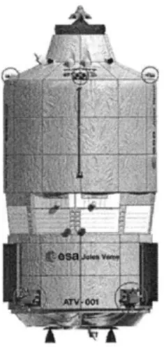
NASA's Cassini spacecraft is a simple example of an overactuated spacecraft with redundancy [23]. For example, if one of the main bi-propellant engines, shown in Figure 2-1, fails, the second can be used as a direct replacement to the failed engine. Another example is ESA's Automated Transfer Vehicle (ATV) that uses 28 thrusters for attitude control [24), shown in Figure 2-2.
Figure 2-1: NASA's Cassini spacecraft Figure 2-2: ESA's Automated Transfer Ve-with direct redundancy. hicle with functional redundancy.
For overactuated spacecraft, if a thruster failure occurs, a reconfigurable control allocator is typically used to reallocate any control that would be acutated by the failed thruster to other thrusters that can provide the same control. There is a large body of literature on this topic, which is discussed further in Section 4.2. Wilson provides an interesting extension to this work which utilizes ideas from neural net-works to reconfigure a control allocator in the event of a failure [25]. The neural network takes in the thruster firing commands and the resulting accelerations to per-form a system identification. This inper-formation allows the neural network to "train"
'This definition is somewhat ill-defined. There are saturation limits that make it impossible to produce an arbitrary force and torque. A more technically correct definition is that there are more actuators than necessary such that the convex hull of the set of forces and torques generated by the feasible control inputs contains the origin.
the control allocator to give better commands to produce the desired accelerations. This system was shown to be able to recover from failed-off thrusters as well as large thruster misalignments.
Thruster failure recovery for underactuated spacecraft has received some attention in the literature as well. Tsiotras and Doumtchenko provide an excellent review of work done in the area of underactuated attitude control of spacecraft [26]. Of note is work by Krishnan, Reyhanoglu, McClamroch which uses a discontinuous feedback controller to stabilize a spacecraft's attitude using only two control torques about the principal axes [27]. Controllability and stabilizability properties are provided for the spacecraft attitude dynamics for an axially and non-axially symmertic spacecraft and it is shown that the dynamics cannot be asymptotically stabilized using continuous feedback. A discontinuous feedback controller is constructed by switching the contin-uous feedback controller used, following a sequence of maneuvers. This is shown to be able to arbitrarily reorient the spacecraft's attitude. In all of these references, the control inputs are considered to be torques provided by pairs of thrusters or reaction wheels.
Failure recovery for the translational degrees of freedom have also been covered to a more limited extent in the literature. Breger developed maneuvers that are safe to thruster failures during the spacecraft docking [28]. Model predictive control is employed to ensure that there is a passive or active trajectory that the spacecraft can follow in the event of a thruster failure, to avoid a collision. This framework does not address the ability of the spacecraft to regulate its position about an equilibrium, but rather the ability to avoid a collision with the spacecraft to which it is docking. The control inputs are assumed to be forces provided by thrusters acting through the spacecraft's center of mass.
2.3
Gap Analysis
A review of the literature for thruster FDIR has been provided. Several methods
type of failure (bank of Kalman filters) as well as methods developed specifically for thruster failures (maximum likelihood and motion-based FDI). From this review, it is concluded that thruster FDI is a solved problem. The motion-based FDI algorithm provides fast detection and isolation of thruster failures and has been proven in space on the SPHERES testbed [291.
While thruster failure recovery has also been addressed in the literature, there is gap that has not been addressed directly. The most common technique for thruster failure recovery is through the use of a reconfigurable control allocator, typically used for overactuated spacecraft. Techniques for controlling the attitude of underactuated spacecraft have also been developed with less than three control torques. In addition, translational control techniques have been developed to avoid collisions and applied to failure scenarios during docking. However, techniques for controlling the attitude
and position underactuated spacecraft have not been discussed in the literature. This
is because attitude is normally independent of position. Satellites mostly control their attitude to point to targets to collect measurements, communicate to ground stations, and collect energy from the Sun. Translational control is activated infrequently and often in an open-loop fashion as it is only required during specific times such as orbit insertion and stationkeeping. Therefore, attitude and position can be treated independently. For satellites in a formation or cluster, however, attitude and position need to be controlled constantly to maintain the formation and avoid collisions. A control system that is able to stabilize the spacecraft about a certain attitude and position in the event of thruster failures has not been developed previously.
Chapter 3
Spacecraft Model
Before developing a control system that is able to handle thruster failures, a dynamic model of the spacecraft must first be developed and analyzed. This chapter is split into three main sections. Section 3.1 provides background material on rigid-body dynamics, which forms the basis for the equations of motion of a thruster-controlled spacecraft given in Section 3.2. Finally, Section 3.3 analyzes the controllability of a representative spacecraft described in Section 1.2, revealing the important char-acteristics about the spacecraft. Standard linear controllability analysis shows that the linearized system is not controllabile in the event of thruster failures. A non-linear controllability test is applied to the spacecraft, showing that the presented representation of the system is also not small-time locally controllable (STLC) in the event of thruster failures. In addition, this analysis shows that the system, with failed thrusters, is underactuated and therefore second-order nonholonomic. Knowing these properties will become useful in the design of a reconfigurable controller for this system.
3.1
Rigid-Body Dynamics
This section provides a brief overview of rigid-body dynamics, the basic equations of motion of a spacecraft. Section 3.1.1 provides a description of reference frames and rotations, a fundamental concept for describing concepts such as spacecraft attitude.
Sections 3.1.2 and 3.1.3 derive the basic kinematic and kinetic equations of motion for the attitude and translational dynamics of a spacecraft.
3.1.1
Reference Frames & Rotations
Reference frames are useful for expressing vectors (a mathematical abstraction with a magnitude and direction) as concrete quantities that can be manipulated. A vector can be represented in a particular reference frame as a linear combination of the unit vectors, forming the axes, of the reference frame. The two reference frames that will be used extensively are the inertial frame, F, and the body frame, FB.
The inertial frame is a special frame of reference in which Newton's laws of motion apply, without modification. Many frames of reference are not truly inertial frames, but can be approximated as such when the fictitious forces due to the use of a non-inertial frame of reference are negligible. The axes of the non-inertial frame are denoted
by three dextral (right-handed), orthonormal unit vectors ii, .2 and i3. The body frame is fixed relative to the spacecraft's geometry with axes bi, b2 and 63. These unit vectors are referred to as basis vectors. A rigorous, mathematical definition of reference frames using vectricies (useful for deriving many of the equations presented) is recommended for further reading [30].
Column matricies are used to collect the components of a vector expressed in a particular reference frame. In other words, a column matrix is a vector expressed in a particular reference frame. It is often necessary to convert a column matrix from one reference frame to another. Conversion of a column matrix in FB, CB E R3, to a column matrix in Fj, c, E R3, is done by left multiplying it with a rotation matrix,
o
E R3x3, that transforms column matricies from YF to YB:CB ~ 9CI (3-1)
This rotation matrix is also called a direction cosine matrix because each element in 1 is &ij = cos Oig, where Bij is the angle between ii and bj. A useful property of this
matrix, since it is orthonormal, is that its inverse is its transpose:
9-1 = 1T. (3.2)
Thus, to transform a column matrix from FB to F,
C, = eT CB- (3-3)
The direction cosine matrix, since it relates two reference frames, can be used to represent the attitude of a spacecraft. However, the attitude of a spacecraft can be expressed with as few as three variables compared to the nine in a direction cosine matrix. Euler angles, a parameterization using three simple rotations, is commonly used because it is easy to visualize. However, this parameterization has geometric singularities that cause the loss of a degree of freedom or 'gimbal lock' at certain angles depending on the sequence of rotations. This also leads to kinematic singu-larities where Euler angle rates can become very large at these angles for relatively small angular rates. While it is possible to avoid these singularities, for example by switching between different rotation sequences when a singularity is approached, the complexity greatly outweighs simply using another parameterization. While there are other attitude parameterizations, the one that shall be used from here on is the unit quaternion or Euler parameters.
The unit quaternion has gained significant use in spacecrafts due to its lack of geometric and kinematic singularities, its ease of use for multiple successive rotations
[31],
and smaller computational load[32]
since it has the lowest number of parame-ters whose kinematic equations do not contain trigonometric functions (see Section3.1.2 for more information on the quaternion kinematic equations). The quaternion
contains four parameters,
- - T
q A qi q2 q3 g4 . (3.4)
These parameters are derived from Euler's Theorem, which loosely states that any rotation can be described by a rotation of angle, 0, about some axis, a. This axis is
invariant in both reference frames (i.e., a = Oa)1 and therefore the arrow denoting a vector can be dropped without ambiguity since it is equally valid in both reference frames. The first three parameters of a quaternion are defined as,
q13 =[ i q2 q31T a sin (3.5)
and the fourth is defined as,
0
q4 cos -. (3.6)
2
Because four parameters are being used to parameterize three degrees of freedom, a constraint must be introduced. The constraint is that the quaternion must be unit length,
/ = g ++ 1. (3.7)
From here on, the unit quaternion will be referred to simply as the quaternion, and the unit length constraint will be implied. Since the direction cosine matrix is still useful in transforming column matricies, it can be calculated from the quaternion by
[30, 31]: 0(q) = (q2 - q Tq13)I3x3 + 2qi3q T - 2q4qi (3.8a) q q - - gq + q2 2(qlq2 + q3q4) 2(q1q3 - q2q4) -1 2 2 2 = 2(qiq2 - q3q4) -q + q2 - q + q4 2(q2q3 + qiq4) (3.8b)
2(qq
3+ q
2q
4)
2(q
2q
3- qi q
4)
-q
-
2 +q I+
q2where the x superscript denotes the 3 x 3 the skew-symmetric cross-product matrix associated with the 3 x 1 column matrix. In general,
ai
0
-a
3
a
2
a= a2 -a a3 0 -ai (3.9)
a3 -a2 ai 0
For attitude estimation and control, it is useful to define an error quaternion that
represents a rotation from one attitude to another. The rotation from a given reference quaternion, qr to the current quaternion, qc, is defined by the error quaternion
[33],
qr4 gr3 -qr2 -qr1 qc1
[qc13qr13 + gr4qc13 - c-r3 qr4 qrl -qr 2 qc2 (3.10)
[
~qc13 '13 + qc4qr4 qr2 -qr 1 qr4 -qr3 qc3qr
1 qr2Gr
3 qr4 qc4Now that reference frames, rotations between reference frames and the quater-nion parameterization have been presented, the dynamic equations that describe the motion of a rigid body will be developed as a model of a spacecraft.
3.1.2
Attitude Kinematics & Kinetics
With the description of attitude using direction cosine matricies and quaternions, it is now necessary to describe how attitude changes over time. This is the study of kinematics, which relates angular velocity and attitude as well as velocity and position. If FB is rotating with respect to
r,
then wBI, is the angular velocity ofYB with respect to Fr. It is most common to express LJBJ in YB since
'strapped-down' rate gyros can directly measure these quantities. All further references of the angular velocity column matrix, o = w W2 W3 T, is the angular velocity of FB
with respect to F, expressed in YB.
Using this idea of angular velocity and a quaternion, q, representing a rotation from YB to Y, the kinematic equation for attitude can be expressed as [30, 34],
q4w1 - q3w2
+
q2W31 1 1 q3 1
+q
402--
(13q = -Q(q)w = --O(w)q - (3.11)
2 2 2 -q2wq1 w12
+q
4 3where R(w) and Q(q) are defined2 as
-~) -~-- -- - (3.12a)
q3
+
q4I
Q(q)
---.
(3.12b)
~q13
When Equation 3.11 is integrated numerically, the quaternion will no longer satisfy the unit constraint of Equation 3.7 after a few integration steps due to rounding errors. The quaternion can be normalized periodically to satisfy this constraint [35].
Knowing the kinematics involved with quaternions, the kinetics, or how this mo-tion arises due to forces, can now be studied. The kinetic equamo-tions can be derived from Euler's law:
h=F (3.13)
where h is angular momentum of the center of mass and i' is the sum of the external torques applied to the rigid body. It is important to note that the dot represents the time derivative with respect to an inertial frame. Therefore, when the derivative is taken with h Jw and i expressed in FB, an extra term appears:
h+ wh = r (3.14)
where J E R"x is the second moment of inertia or the inertia matrix about the center of mass expressed in FB. Assuming that J is constant, this equation becomes
W = -Jlw x Jw + J%'r. (3.15)
This equation, along with the Equation 3.11, can be integrated to determine the angular motion of a rigid body subject to torques.
2These two definitions, S? and Q,
3.1.3
Translational Kinematics & Kinetics
In addition to the attitude dynamics, the translational dynamics of a rigid body must also be described. The position, r', of a rigid body is a vector from the origin of F to the origin of TB. The kinematic equations relating the position and velocity, i, of a rigid body is simply
r= V. (3.16)
When ' and V are expressed in F1,3 this equation becomes
r = V. (3.17)
The kinetic equations can be derived from Newton's Second Law:
(3.18)
where p = mu + WJ x C' is the linear momentum of a rigid body, m is the mass of the rigid body, ' is the first moment of inertia with respect to the origin of FB and
f
is the net external force acting on the rigid body. Assuming that the origin is the center of mass (C'= 0) and m is constant, the equation of motion expressed in Fh becomes1 v =-f
m (3.19)
3.2
Equations of Motion of a Thruster-Controlled
Spacecraft
With the equations of motion of a rigid body given in Equations 3.11, 3.15, 3.17 and
3.19, a model of a thruster-controlled spacecraft can be developed. The full
six-degree-of-freedom (6DOF) model is given in Section 3.2.1, which models the dynamics of a
3This may seem trivial but it is important to note that the dot is the time derivative with respect
to an inertial frame. Thus, if r were expressed in FB, an w r term would appear, similar to
Equation 3.14.
thruster-controlled spacecraft with three translational and three rotational degrees of freedom. In addition, a reduced three-degree-of-freedom (3DOF) model is given in Section 3.2.2, which models the dynamics of a spacecraft restricted to a plane with two translational degrees of freedom and one rotational degree of freedom. This
3DOF model is useful for exploring concepts in a simpler setting before jumping into
the full six-degree-of-freedom model.
3.2.1
Six-Degree-of-Freedom Model
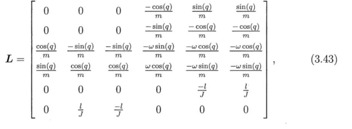
Thrusters are modeled as a body-fixed force that is applied to a set location on the spacecraft. The lever arms and thrust directions of all m thrusters4 can be arranged in matricies of size 3 x m The thruster lever arms are given by
L = [11 12 ... 1,n (3.20)
where i E R3 represents the column matrix describing the lever arm of the ith thruster
in FB. The thrust directions are given by
D = [d d2 ... dm-] (3.21)
where di E R3 represents the column matrix describing the direction of the ith thruster in FB. The force provided by each thruster is given by a column matrix U E [0, uma)"'. It is important to note that these thruster forces are unilateral,
meaning that they cannot produce negative thrust. The full equations of motion of a thruster-controlled spacecraft are summarized below.
= V (3.22a)
i7 = iT(q)Du (3.22b)
m
4
Because m refers to mass as well as the number of thrusters, the distinction must be made by context.
q = Q- (Lo)q (3.22c)
2
c - l wJlx^Jo + J-Lu (3.22d)
One important feature of Equation 3.22b is that the effect of the thrusters must be rotated from YB to Fr with 0 T given in Equation 3.8. The definitions of the variables
of Equations 3.22a-3.22d are summarized in Table 3.1. The main assumptions of these equations is that the origin of FB is at the center of mass of the spacecraft, and that the spacecraft can be treated as a rigid body (no flexibility/slosh in the spacecraft).
Table 3.1: Variable definitions for the 6DOF model.
Variable Size Reference Frame Description
r 3 x 1 F1 Position of the origin of YB relative to F1
v 3 x 1 Y Velocity of the origin of YB relative to F
q 4 x 1 Rotation from F1 to YB
O 3 x 1 YB Angular velocity of YB relative to F1
9 3 x 3 - Rotation matrix representation of q
f2 4 x 4 YB Kinematic quaternion matrix
m l x I Spacecraft mass
J 3 x 3 YB Spacecraft inertia about the center of mass
L 3 x m YB Matrix of thruster lever arms
D 3 x m YB Matrix of thrust directions
3.2.2
Three-Degree-of-Freedom Model
The 3DOF model represents the motion of a spacecraft restricted to a plane. The spacecraft has two translational degrees of freedom, forming the plane, and one rota-tional degree of freedom normal to said plane. The 3DOF model has a very similar structure to the 6DOF model and the same assumptions. Position, r, and velocity,
v, as well as the columns of the thruster direction matrix, D, are reduced from the
domain R3 to JR2. Attitude, q, angular rate, w, and the columns of the thruster lever arm matrix, L, and are reduced from the domain R3 to R. Attitude is now an angle in the range [-7r, 7r) describing the rotation of from Fr to YB. The corresponding
rotation matrix is given by
9 (q)=
[cos(q)sin(q)
(3.23)- sin(q) cos(q).
With these new definitions, the 3DOF model of a thruster-controlled spacecraft is summarized below. r = v (3.24a) iv = &T(q)Du (3.24b) m t4 = W (3.24c) 1 C -Lu (3.24d)
For convenience, a summary of the variables are summarized in Table 3.2. Table 3.2: Variable definitions for the 3DOF model.
Variable Size Reference Frame Description
r 2 x 1 F: Position of the origin of FB relative to FT
v 2 x 1 F Velocity of the origin of F relative to F1
q 1 x 1 - Rotation from F1 to F
W 1 X 1 FR Angular velocity of FR relative to Fr
9 2 x 2 - Rotation matrix representation of q
m 1 x 1 - Spacecraft mass
J 1 x 1 FB Spacecraft inertia about the center of mass
L 1 x m FB Matrix of thruster lever arms
D 2 x m FB Matrix of thrust directions
3.3
Controllability
Now that the model for a thruster-controlled spacecraft has been developed, it is useful to derive the controllability of this system, which will give valuable insight into its complex nature. The idea of controllability does invoke an intuitive definition, however the exact definition must be clear from a mathematical standpoint. A system is controllable if for all states xi and xf there exists a finite-length control input
trajectory, u(t) : [0, T] - U, such that the solution to the initial value problem
x = f (x,u), x(0) = Xi (3.25)
has the solution x(T) xf. Note that U simply denotes an admissible set of
con-trol inputs. Put simply, a system is concon-trollable if there is a feasible concon-trol input trajectory that can drive the system from any initial state to any final state.
Despite its fundamental role in control theory, a completely general set of condi-tions for controllability of nonlinear systems does not currently exist [36]. For the limited case of linear, time-invariant systems, there is a simple method of determining controllability. This will be discussed in Section 3.3.1, along with the limitations ex-plaining why this analysis does not provide a complete controllability results. Next, a limited nonlinear controllability analysis will be discussed in Section 3.3.2 along with the derived small-time local controllability (STLC) of this system.
3.3.1
Linear Time-Invariant Controllability
Linear, time-invariant (LTI) systems have been studied extensively and there exists a simple test for determining the controllability of an LTI system. The dynamics of any LTI system can be expressed as
x = Ax + Bu (3.26)
where x E R" is the state, u E R"n is the control inputs, A E Rn"" is the dynamics matrix, and B E R"X"m is the input matrix. Controllability of LTI systems can easily be determined by calculating the controllability matrix
Mc = [B AB A2B ... An-1BI. (3.27)
If Mc is full rank, rank(Mc) = n, the system is controllable [37].
This test for determining controllability cannot be used directly on the system given by Equations 3.22a through 3.22d since it is nonlinear. A system with dynamics
expressed as
J; f (x, u) (3.28)
must first be linearized about a certain state, xe, and control input, ue by performing
a Taylor series expansion of
f
about xe and ue. Using only the first-order terms in the expansion, the linearized dynamics can be written as[
OX IXe7Uau
Xe ,Ue6=+6 (3.29)
L ax
XeUej LUau
Xe,UeWhile the system can be linearized, there are a few issues with this approach. The first issue is that the thruster input forces are unilateral, rendering a simple rank check invalid. As a simple example, take the following double-integrator system,
0 1 0
X + U, (3.30)
L0 0 1L1
where u E [0, oo) is a unilateral control input'. Physically, this system can represent a spacecraft, with a single thruster, whose motion is restricted to one translational degree of freedom. Obviously, the system is not controllable since it can only fire its thruster in a single direction and can therefore only accelerate in a single direction. To be controllable, the spacecraft would need two thrusters pointing opposite directions, which effectively eliminates the unilateral constraint on the control input. While this conclusion is relatively straightforward, determining this mathematically is more challenging. The controllability matrix for this system is
-0 1
Mc = [B AB] = . (3.31)
If the rank condition is blindly applied to this matrix, one would incorrectly conclude that the system is controllable since the matrix is full rank. This is because the
![Figure 1-1: Distribution of attitude and orbit control system failures [2].](https://thumb-eu.123doks.com/thumbv2/123doknet/14137431.469873/16.918.241.713.742.1004/figure-distribution-attitude-orbit-control-failures.webp)
![Figure 1-2: Artist's conception of DARPA's System F6 [9].](https://thumb-eu.123doks.com/thumbv2/123doknet/14137431.469873/18.918.184.753.573.977/figure-artist-s-conception-darpa-s-f.webp)

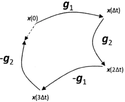
![Figure 3-3: Differential drive example showing a series of four motion primitives [39].](https://thumb-eu.123doks.com/thumbv2/123doknet/14137431.469873/47.918.238.695.676.934/figure-differential-drive-example-showing-series-motion-primitives.webp)