Practical Considerations of Deploying AI in Defect Prediction: A Case Study within the Turkish Telecommunication Industry

Publisher’s version / Version de l'éditeur:

Proceedings of the International Conference on Predictor Models in Software

Engineering, 2009-05-17

READ THESE TERMS AND CONDITIONS CAREFULLY BEFORE USING THIS WEBSITE. https://nrc-publications.canada.ca/eng/copyright

Vous avez des questions? Nous pouvons vous aider. Pour communiquer directement avec un auteur, consultez la première page de la revue dans laquelle son article a été publié afin de trouver ses coordonnées. Si vous n’arrivez pas à les repérer, communiquez avec nous à PublicationsArchive-ArchivesPublications@nrc-cnrc.gc.ca.

Questions? Contact the NRC Publications Archive team at

PublicationsArchive-ArchivesPublications@nrc-cnrc.gc.ca. If you wish to email the authors directly, please see the first page of the publication for their contact information.

NRC Publications Archive

Archives des publications du CNRC

This publication could be one of several versions: author’s original, accepted manuscript or the publisher’s version. / La version de cette publication peut être l’une des suivantes : la version prépublication de l’auteur, la version acceptée du manuscrit ou la version de l’éditeur.

Access and use of this website and the material on it are subject to the Terms and Conditions set forth at

Practical Considerations of Deploying AI in Defect Prediction: A Case

Study within the Turkish Telecommunication Industry

Tosun, Ayse; Turhan, Burak; Bener, Ayse

https://publications-cnrc.canada.ca/fra/droits

L’accès à ce site Web et l’utilisation de son contenu sont assujettis aux conditions présentées dans le site LISEZ CES CONDITIONS ATTENTIVEMENT AVANT D’UTILISER CE SITE WEB.

NRC Publications Record / Notice d'Archives des publications de CNRC:

https://nrc-publications.canada.ca/eng/view/object/?id=da581cec-ab62-4c8f-aef3-ce9bea0a2644

https://publications-cnrc.canada.ca/fra/voir/objet/?id=da581cec-ab62-4c8f-aef3-ce9bea0a2644

Practical Considerations in Deploying AI for Defect

Prediction: A Case Study within the Turkish

Telecommunication Industry

Ayşe Tosun

Department of Computer Engineering,

Boğaziçi University, Istanbul, Turkey +90 212 359 7227

ayse.tosun@boun.edu.tr

Burak Turhan

Institute for Information Technology National Research Council,

Ottawa, ON, Canada +1 613 993 7291

Burak.Turhan@nrc-cnrc.gc.ca

Ayşe Bener

Department of Computer Engineering,

Boğaziçi University, Istanbul, Turkey +90 212 359 7227

bener@boun.edu.tr

ABSTRACT

We have conducted a study in a large telecommunication company in Turkey to employ a software measurement program and to predict pre-release defects. We have previously built such predictors using AI techniques. This project is a transfer of our research experience into a real life setting to solve a specific problem for the company: to improve code quality by predicting pre-release defects and efficiently allocating testing resources. Our results in this project have many practical implications that managers have started benefiting: code analysis, bug tracking, effective use of version management system and defect prediction. Using version history information, developers can find around 88% of the defects with 28% false alarms, compared to same detection rate with 50% false alarms without using historical data. In this paper we also shared in detail our experience in terms of the project steps (i.e. challenges and opportunities).

Categories and Subject Descriptors

D.2.9 [Management]: Software Quality Assurance. D.4.8 [Performance]: Measurements, Modeling and Prediction.

General Terms

Measurement, Prediction.

Keywords

Software defect prediction, AI methods, experience report, static code attributes.

1.

INTRODUCTION

Telecommunications is a highly competitive and booming industry in Turkey and its neighbours. The leading GSM operator in Turkey operates in Azerbaijan, Kazakhstan, Georgia, Northern Cyprus and Ukraine with a customer base of 53,4

million. The company has grown very rapidly and successfully since its inception in 1994. It has an R&D centre having 200 researchers and engineers with 1 to 10 years of experience. Their legacy software has millions of lines of code that needs to be maintained.

The company is under constant pressure to launch new and better campaigns in limited amount of time with tight budgets. As the technology changes and the customers require new functionalities, they have to respond faster than ever by means of new software releases. Currently, they make releases in every two weeks. They use incremental software development [21], where each release has additional or modified functionalities, compared to the previous releases. So there is a limited time to track, control and fix the problems in their software. Similar to other software development companies, testing is one of the most critical stages in their development cycle [2, 12, 14]. Accordingly, the managers seek to lever any opportunity for improving their software development.

Our study involved in construction of a metrics program and a decision support system to predict defects and apply more effective release management. Previous studies have implemented extensive automated metrics and defect prediction programs using data mining, specifically at NASA [1]. In this paper, we describe our experience in translating those programs to a telecommunication company. While the company‟s development practices are very different from those of NASA, the automated AI methods ported with relatively little effort. However, we spent much time learning the organization and working within their current practices. In that respect, we present our experience on the practical applications of AI techniques to solve the problems of the company‟s software development processes. The results of our study showed thatpractitioners can benefit from a learning-based defect predictor on the allocation of resources, bug tracing and measurement in a large software system. Using code metrics and version history, we managed to keep high stable detection rates, on the average 88%, while decreasing false alarms by 44%. Those improvements in the classification accuracy also affected the estimated inspection costs of testers to detect defective modules.

2.

GOALS OF THE PROJECT

Our goals in this project are defined as building a code measurement, bug tracing/ matching program and a defect prediction model. We have jointly agreed on these goals with the

Permission to make digital or hard copies of part or all of this work or personal or classroom use is granted without fee provided that copies are not made or distributed for profit or commercial advantage and that copies bear this notice and the full citation on the first page. To copy otherwise, to republish, to post on servers, or to redistribute to lists, requires prior specific permission and/or a fee.

R&D manager, project managers and development team during the project kick-off meeting. Furthermore, senior management strongly believed that they should adjust their development processes to increase software quality as well as to make efficient resource allocation. We have decided on the roles and responsibilities and aligned the goals of the project with their business goals (Table 1). We clearly explained to them what they will have at the end.

Table 1. Goals in line with business objectives Goals of the project Management objectives Code measurement and

analysis of the software system.

-Improve code quality

Construction of a defect prediction model to predict defect prone modules before testing phase.

-Decrease lifecycle costs such as testing effort. -Decrease defect rates

Storing a version history and bug data.

-Measure/ control the time to repair the defects

In order to track the progress of the project, we decided to make monthly meetings with the project team, and quarterly meetings with the senior management to present the progress and discuss on the next step. Senior management meetings were quite important either to escalate the problems or to get their blessing on some critical decisions we had to make throughout the project. During the life of the project, Softlab researchers were on-site on a weekly basis to work with the coders, testers and quality teams. Previously, the company did not employ any measurement processes due to tight schedules and heavy workloads. Therefore, we have planned our work in four main phases. In the first phase, we aimed to measure static code attributes at functional/ method level from their source code. In the second phase, we planned to match software methods with pre-release defects. In the third and fourth phases, we planned to build and calibrate a defect prediction model, assuming that we would be able to collect enough data to train our model. However, the outcomes of every phase have led us to re-define and extend the original scope and objectives in the later stages. In the next sections, we will explain our initial plans, challenges we come across during each phase and our methodology to solve these problems in detail.

3.

PHASE I: CODE MEASUREMENT AND

ANALYSIS

In the first three months of the project, we aimed to analyze the company‟s coding practices and to conduct a literature survey of measurement and defect prediction in the telecommunications industry. At the end of this phase, we aimed at having agreed on the list of static code attributes and to decide on an automatic tool to collect them. We also hoped to have collected the first set of static code attributes from the source code in order to make a raw code analysis. In order to do that, we would choose the sample projects that we would collect data from.

We decided that static code attributes can be used to point out current coding practices. Static code attributes are accepted as reliable indicators of defective modules in the software systems.

They are widely used [1, 3, 6, 12, 15, 16, 17, 18] and easily collected through automated tools. Therefore, we have defined the set of static code attributes from NASA MDP Repository [12], as the metrics to be collected from the software in the company. Basically, we collected complexity metrics proposed by McCabe [5], metrics related to unique number of operators and operands, which are proposed by Halstead [4], size metrics to count executable and commented lines of code, and CK object-oriented metrics [19] from Java applications. Due to lack of space, we could not publish the set of metrics collected from their software. However, we have donated all data that comes from nine applications of the software to the Promise Repository [7] in terms of method, class, package and file levels. So they are publicly available for replicated studies or new experiments.

3.1

Challenges during Phase I

As mentioned earlier, the company did not have a process or an automated tool to measure code attributes. Our suggestion was to buy a commercially available automated tool to extract metrics information easily and quickly. However, due to budget constraints and concerns for adequacy of functionalities of the existing tools, senior management did not want to make an investment on such a tool. Besides, their software systems contain source codes and scripts written in different languages such as Java, JSP. Therefore the management was not convinced to find a cost effective single tool that would embrace all languages and extract similar attributes easily from all of them.

Software system has the standard 3-tier architecture with presentation, application and data layers. However, the content in these layers cannot be separated as distinct projects. Any enhancement to the existing software somehow touches all or some of the layers at the same time, making it difficult to identify code ownership as well as to define distinct software projects. Another problem we have come across was related with the metrics collection process. When we observed the software development process with coding practices of the team, it seemed that collecting static code attributes in the same manner with NASA datasets, i.e. in functional method level, is almost impossible due to lack of an available automated mechanisms that would match those attributes with the defect data.

3.2

Our Methodology

Metric Extraction: We have implemented an all-in-one metrics extraction and analysis tool, Prest, to extract code metrics [9]. Compared to other commercial and open source tools, Prest embraces many distinctive features and it is freely available. It extracts 22 to 26 static code attributes in different granularities, i.e. package, class, file, method level. It is able to parse programming languages such as C, C++, Java, JSP, PL/SQL, and forms a dependency matrix that keeps inter-relations between modules of the software systems. Prest has a simple user interface, where the user can import the source code and parse his/her project using one or more language parsers. It is able to parse different parts of the code, using parsers of different programming languages (Figure 1). Then, static code attributes extracted in four granularity levels are displayed on the screen. Additional analysis on modules helps to identify critical modules whose attributes do not meet the coding standards of NASA MDP [12]. Sample screenshot for a GSM project can be seen in Figure 2.

Figure 1. Screenshot from Prest: Parsing a project

Figure 2. Screenshot from Prest: Displaying results We were able to collect static code attributes from 22 critical applications of the company. Moreover, we have inserted defect labels, i.e., 1 for defective and 0 for defect-free, to the modules using the UI. Then, we converted them to arff format to use in the classifier component of the tool. Currently, classifier component of Prest applies Naïve Bayes and Decision Tree algorithms, from which we have used the former one as the algorithm of our predictor.

Project Selection: This was one of our first critical decisions in this project in order to define the scope and to choose projects and/ or units of production that would be under study. Although project managers initially wanted to focus on presentation and application layers due to the complexity of the architecture, we jointly decided to take 22 critical and highly interconnected Java applications embedded in these layers. We refer to them as projects during this study.

Level of granularity: As we mentioned in the previous section, we were unable to use method-level metrics in the software system, since we could not collect method-level defect data from the developers in such limited amount of time. Therefore, we have aggregated our method-level attributes to the file-level by taking minimum, maximum, average and sum values of each file [17] in order to make them compatible with defect data.

4.

PHASE II: BUG TRACING AND

MATCHING

The second phase of our study was originally planned to store defect data, i.e. test and production defects. If things had their

normal course of action in Phase I, we would have collected metrics from the completed versions of 22 projects and matched the bugs as well.

4.1

Challenges during Phase II

This phase took much longer than we anticipated. First of all, there was no process for bug tracing. Secondly, test defects were not stored at method level during development activities. Thirdly, there was no process to match bugs.

The project team has realized that the system is very complex such that it needs too much time and effort to match each defect with its file constantly. Additionally, developers did not volunteer to participate in this process, since keeping bug reports would have increased their busy workloads.

4.2

Our Methodology

To solve these issues, we called for an emergency meeting with senior management as well as with the heads of development, testing and quality teams. As a result, the company agreed to change their existing code development process. They built a version control log to keep changes in the source code done by the development team. These changes can be either bug fixing or new requirement request, all of which are uniquely numbered in the system. Whenever a developer checks in the source code to the version control system, he/she should provide additional information about the modified file, i.e. id of test defect or requirement request. Then, we would be able to retrieve those defect logs from the history and match them with the files of the projects in that version. We manually combined static code attributes with a defect flag, indicating 1 for defective files and 0 for defect-free files. This process change also enabled the company to establish code ownership.

During adaptation of this process change, we did additional analysis on static code attributes to point out some of the problems in the coding practices of the company‟s development team. Our intention was to represent the software development practices in the company, mention critical aspects and convince the team and the managers for those required course of actions. We have taken best practice coding standards of NASA MDP Repository [12] and compared them with our measurements. Based on our analysis, we have seen that there are two fundamental issues in the coding practices: a) No comments at all, which makes the source code hard to read and understand by other developers, b) Limited usage of vocabulary, which brings that the system is unnecessarily modular due to JSP codes from the application layer. This code analysis supports the necessity to improve the software quality.

Moreover, as an alternative analysis, we have conducted a rule-based code review process, rule-based on code metrics. Our aim here was to present what amount of code should be reviewed and how much testing effort is needed to inspect defect-prone modules in the company [14]. To do this, we have simply defined rules for each attribute, based on its recommended minimum and maximum values [12]. These rules are fired, if a module‟s selected attribute is not in the specified interval. This also indicates that the module could be defect-prone, therefore, it should be manually inspected. The results of the rule-based model can be seen in Figure 3, where there are 17 basic rules with the corresponding attributes and two

additional rules derived from all of the attributes. Rule #18 is fired if any of 17 rules is fired. This rule shows that we need to inspect 100% LOC to find defect-prone modules of the overall system. Besides, Rule #19 is fired if all basic rules, but the Halstead rules, are fired. This reduces the firing frequency of the former rule such that 45% of the code (341655 LOC) should be reviewed to detect potentially problematic modules in the software.

We have seen that rule-based code review process is impractical in the sense that we need to inspect 45% of the code [14]. So, it is obvious that we need more intelligent oracles to decrease testing effort and defect rates in the software system.

Figure 3. Rule based analysis

5.

PHASE III: DEFECT PREDICTION

MODELLING

The original plan in this phase was to start constructing our prediction model with the data we had been collecting from the projects. We had planned to test the performance of our model with the ones in the literature. We would try different experimental designs, sampling methods, and AI algorithms to build such a model.

We planned to build a learning-based defect predictor for the company. We have agreed to use Naïve Bayes classifier as the learner of this model, since a) it is simple and robust as a machine learning technique, b) it performs the best prediction accuracy, compared to other machine learning methods [1], and c) recent study by Lessmann et al. also shows that most of the machine learning algorithms are not significantly better than each other in defect prediction [18]. We also agreed on the performance measures of the defect predictor that we would build. We decided using three measures: probability of detection, pd, probability of false alarm, pf, and balance from signal detection theory [13]. Pd measures the percentage of defective modules that are correctly classified by the predictor. Pf, on the other hand, is a measure to calculate the ratio of defect-free modules that are wrongly classified as defective with our predictor. In the ideal case, we expect to see {100%, 0} for {pd, pf} rates, however, the model trigger more often which has a cost of false alarms [1]. Finally,

balance indicates how close our estimates to the ideal case by calculating the Euclidean distance between the performance of our model and the point {100, 0}. Obviously, we have computed these measures by comparing our predictions with the actual defect data at every release. A confusion matrix is used to compute performance measures (Table 2) with the formulas.

Table 2. Typical confusion matrix predicted

Actual

defective defect free

defective A B

defect free C D

pd = A / (A + C) pf = B / (B + D)

bal =

₁

_-

₍₀

_-

_pf)



₍₁

_-

_pd)

₂

In order to interpret our results to business managers, we also agreed to construct a cost-benefit analysis based on Arisholm and Briand‟s work [23]. We would simply measure the amount of LOC or the number of modules that our model would predict as defective. Then we would compare this with a random testing strategy to measure how much we gain from testing effort by using our predictor. In a random testing strategy, it is assumed that we need to inspect K percent of LOC to detect K percent of defective modules [23]. Our aim is to decrease this inspection cost with the help of our predictor.

5.1

Challenges during Phase III

Although we started collecting data from completed versions of the software system, we have realized that constructing such a dataset would take a long time. We have seen that building a version history is an inconsistent process. Developers could allocate extra time to write all test defects they fixed during the testing phase due to other business priorities. In addition, matching those defects with corresponding files of the software cannot be automatically handled. We could not form an effective training set for a long time. Therefore, we were not able to build our defect prediction model.

5.2

Our Methodology

Instead of waiting for a complete dataset, we have come up with an alternative way to move ahead. In our previous research, we had suggested companies, like this GSM operator, to build defect predictors with other companies‟ data, i.e. cross-company data [6]. Cross-company data can be used effectively in the absence of a local data repository, especially when special filtering techniques are used:

 Selecting similar projects from cross-company data using nearest neighbor sampling [8].

 Increasing the information content of data using dependency data between modules [22].

In our study, we have selected NASA projects as the cross-company data, which are publicly available [7]. NASA projects contain more than 20.000 modules, of which we used randomly 90% as the training data to predict defective modules in our projects [6]. From this subset, we have selected a subset of projects that are similar to those in our data in terms of Euclidean distance in the 17 dimensional metric spaces [8]. The nearest neighbors in this random subset are used to train the predictor. We have added one more analysis using cross-company data to increase the information content by adding dependency data between modules of the projects. Our previous research [22] shows that false alarms can be decreased from 30% to 20% using a call graph based ranking framework in a public embedded software data [7]. Therefore, we have also included caller-callee relations between modules of NASA and the GSM projects to adjust code metrics with this framework. We repeated this procedure 20 times and raised a flag for modules that are estimated as defective in at least 10 trials [8].

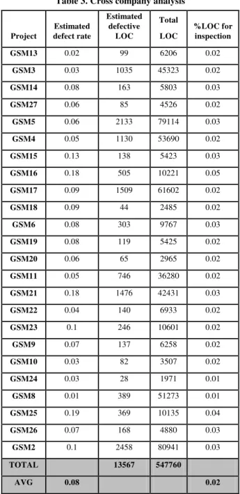
Table 3 shows the results from this analysis on 22 projects. Due to the sizes of projects 7, 23 and 25 and high computing resources, we were unable to derive call graphs for them. Therefore, we left them out of this analysis. Results present the estimated defect rate as 8% in their software system. There is a major difference with the rule based approach in terms of their practical implications. According to the rule-based model, LOC required to inspect corresponds to 45% of the whole code, while module level defect rate is 14%. On the other hand; for the learning-based model, LOC required to inspect corresponds to only 2% of the code, where module level defect rate is estimated as 8%. Therefore, we can once more see the benefits of a learning-based model to decrease testing efforts by guiding testers through defective parts of the software.

The difference between two models is occurred because rule-based model makes decisions rule-based on individual metrics and it has a bias towards more complex and larger modules. On the other hand, learning based model combines all „signals‟ from each metric and estimates defects located in smaller modules [1, 16]. It is important to mention that this analysis was completed in the absence of local data. Therefore, we have used the results to show the tangible benefits of building a defect predictor to the managers and development team in the company.

6.

PHASE IV: DEFECT PREDICTION

EXTENDED

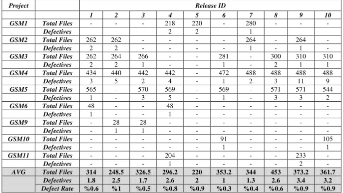
This phase did not exist in our original plan, since we had underestimated the time and effort that was necessary to build a local data repository. In this phase, we were able to collect within-company data from ten versions of the software. Properties of projects in terms of number of files and defect rates are illustrated in Table 4. This data is now at Promise Repository for other researchers to reproduce, refute, and improve our results [7]. We observed discontinuities in projects between releases, since some projects may be rarely deployed or some of them may be withdrawn at a certain release.

Table 3. Cross company analysis

Project Estimated defect rate Estimated defective LOC Total LOC %LOC for inspection GSM13 0.02 99 6206 0.02 GSM3 0.03 1035 45323 0.02 GSM14 0.08 163 5803 0.03 GSM27 0.06 85 4526 0.02 GSM5 0.06 2133 79114 0.03 GSM4 0.05 1130 53690 0.02 GSM15 0.13 138 5423 0.03 GSM16 0.18 505 10221 0.05 GSM17 0.09 1509 61602 0.02 GSM18 0.09 44 2485 0.02 GSM6 0.08 303 9767 0.03 GSM19 0.08 119 5425 0.02 GSM20 0.06 65 2965 0.02 GSM11 0.05 746 36280 0.02 GSM21 0.18 1476 42431 0.03 GSM22 0.04 140 6933 0.02 GSM23 0.1 246 10601 0.02 GSM9 0.07 137 6258 0.02 GSM10 0.03 82 3507 0.02 GSM24 0.03 28 1971 0.01 GSM8 0.01 389 51273 0.01 GSM25 0.19 369 10135 0.04 GSM26 0.07 168 4880 0.03 GSM2 0.1 2458 80941 0.03 TOTAL 13567 547760 AVG 0.08 0.02

We have decided on the experimental design of the local prediction model in Phase IV. First, we have challenged the amount of data, i.e. the ratio between defective and defect-free modules, needed to establish predictions. We chose “micro-sampling” approach based on our previous study [3] and we formed the training set with N defective and M defect-free files such that total size is twice the number of defective modules. Second, we discussed on training data of the model to predict defective files of the projects in the next release. We have conducted two experiments to decide on the best strategy.

Table 4. General properties of GSM projects Project Release ID 1 2 3 4 5 6 7 8 9 10 GSM1 Total Files - - - 218 220 - 280 - - - Defectives 2 2 1 GSM2 Total Files 262 262 - - - - 264 - 264 - Defectives 2 2 - - - - 1 - 1 - GSM3 Total Files 262 264 266 - - 281 - 300 310 310 Defectives 2 2 1 - - 1 - 2 1 1 GSM4 Total Files 434 440 442 442 - 472 488 488 488 488 Defectives 3 5 2 4 - 1 2 3 11 9 GSM5 Total Files 565 - 570 569 - 569 - 571 571 544 Defectives 1 - 3 5 - 1 - 3 3 2 GSM6 Total Files 48 - - 48 - - - - Defectives 1 - - 1 - - - - GSM9 Total Files - 28 28 - - - - Defectives - 1 1 - - - - GSM10 Total Files - - - 91 - - - 105 Defectives - - - 1 - - - 1 GSM11 Total Files - - - 204 - - - - 233 - Defectives - - - 1 - - - - 2 -

AVG Total Files 314 248.5 326.5 296.2 220 353.2 344 453 373.2 361.7 Defectives 1.8 2.5 1.7 2.6 2 1 1.3 2.6 3.4 3.2 Defect Rate %0.6 %1 %0.5 %0.8 %0.9 %0.3 %0.4 %0.6 %0.9 %0.9 Initially, we have used the latest previous release of each project

as the training set, i.e. the latest release that a project was deployed and its metrics as well as defect data were collected. As the second alternative, we have treated the latest previous release of all projects as the training set [14].Test data is the next release of that project, in which development phase has just been completed and testing phase beings. Table 5 shows a sample of two versions and two projects in our experiment results. We have conducted 100 iterations and at each iteration we randomly selected M defect-free files from previous releases to form the training set and predict defect-prone parts of the current release (test set). We took the average performance of 100 iterations. It is observed that both of the approaches produced high pd rates in the range between 78% to 100%. Third column (version-level) presents the prediction performance when we choose our training set from all projects of the previous version to predict defective modules of projects, GSM3 and GSM4. The last column (project-level), on the other hand, shows the performance of our predictor when we use only the previous version of GSM3 or GSM4 to predict defective modules of the selected project in the current version. Results shows that project-level defect predictor is better (bold cells in Table 5), although we have high false alarm rates.

Table 5. Results for version- vs. project-level prediction

Release number Appl. Name 1st experiment with 8 appl. 2nd experiment with GSM 3 or 4 Pd pf bal pd pf bal 2 GSM3 100 67 53 85 34 68 GSM4 78 75 44 80 66 51 3 GSM3 92 51 60 100 36 75 GSM4 81 63 45 90 71 44

6.1

Challenges during Phase IV

The results of this analysis, in Table 5, show that we still produced high false alarms by selecting the training data from previous versions of the specific project only, compared to results, when training data is selected from the previous versions of the various projects in the software. False alarms are dangerous for such local predictors, since they cause the developers or testers inspecting more modules than necessary. This, in fact, contradicts with one of the initial aims of constructing a defect predictor: decreasing testing effort. Since false alarms produce additional costs, it is hard to adopt our predictor to their real development practices. Therefore, we should find a strategy to detect as much defective modules as possible, while decreasing false alarms to a reasonable cost.

6.2

Our Methodology

We have discussed on the reasons of high false alarms in monthly meetings with the project team and found that we need to clean files that are not changed since January 2008 from the version history. For this, we built a simple assumption on defect-proneness of a module: It is highly probable that a module is defect free if it has not been changed since January 2008. Then, we have added a flag to each file of the projects that indicates whether the file is actively changed or passive since January. The model controls each of its predictions by looking at the history flag of these files. If the model predicts a file as defective, although it has not been used since January, then it is re-classified as defect-free.

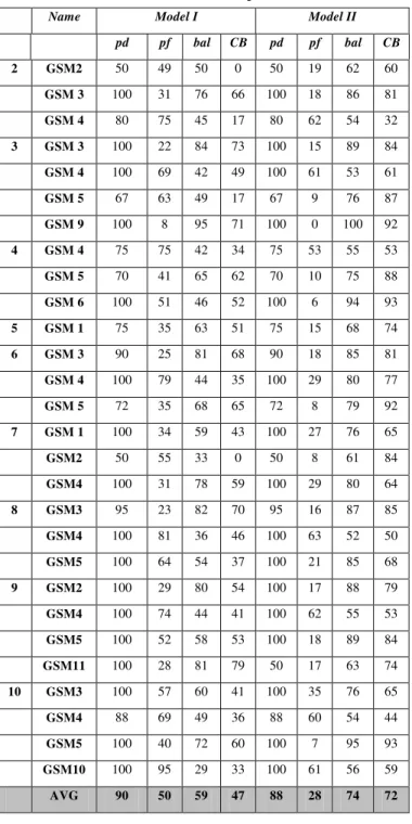
Results of our experiments using only code metrics (Model I) and using code metrics along with history flags (Model II) are summarized in Table 6 for all public datasets. We can clearly observe that using version history improves the predictions

significantly in terms of pf rates. Our model succeeded in decreasing false alarms, on the average from 50% to 28% using version history. The change in pf rates vary in terms of projects in the range of {0%, 63%} due to discontinuities in the changed projects throughout version history. Additionally, we managed to have stable high pd rates, on the average 88%, while reducing pf rates successfully. Besides, we have spent less effort to detect 88% of these defective modules: Cost benefit analysis (CB column in Table 6) shows that we have managed to decrease the inspection effort to detect defective modules by 72%, from 88% to 25%. As a result, using a defect prediction model enables developers allocate their limited amount of time and effort to only defect-prone parts of a system. Managers can also see the practical implications of such decision making tools which reduces testing effort and cost.

We have successfully built our defect predictor for the company using local data and presented our results to the project team. The results of the project showed that the company‟s business goal of decreasing testing effort without compromising the level of product quality can be achieved with intelligent oracles. We have used several methods to calibrate the model for the company in order to get the best prediction performance for them. We have seen that file-level call graph based ranking (CGBR) method did not work due to their transition to Service Oriented Architecture (SOA). SOA did not allow us to capture caller-callee relations through simple file interactions. Moreover, we have only used static code attributes from Java files to build our model. However, there are many PL/ SQL scripts that contain very critical information on the interactions between application and data layers. Thus, a simple call-graph based ranking in file-level could not capture the overall picture and hence fail to increase the information content in our study.

7.

LESSONS LEARNED

During this project we had many challenges to overcome, and we constantly re-defined our processes, and planned for new sets of actions. In this section, we would like to discuss what can be used as best practices, and what needs to be avoided next time. We hope that this study and our self evaluation would shed some light for other researchers and practitioners.

7.1

Best Practices

Managerial Support: From the beginning till the end of this

work, we had full support of senior management, and mid level management. They were available and ready to help whenever we needed them. We believe that without such a support a project like this would not have been concluded successfully.

Project planning and monitoring: One of the critical success

factors was that we had a detailed project plan and we rigorously followed and monitored the plan. This enabled us to identify problems early on and to take necessary precautions on time. Although we had many challenges we were able to finish the project on time achieving and extending its intended goals. These meetings also brought up new and creative research ideas. As a research team we mapped the project plan and its deliverables to new research topics and academic studies. Moreover, the company has gained valuable outcomes, which are described in the next best practice, i.e. “multiplier effect”.

Table 6. Results of local defect prediction model

Name Model I Model II

pd pf bal CB pd pf bal CB 2 GSM2 50 49 50 0 50 19 62 60 GSM 3 100 31 76 66 100 18 86 81 GSM 4 80 75 45 17 80 62 54 32 3 GSM 3 100 22 84 73 100 15 89 84 GSM 4 100 69 42 49 100 61 53 61 GSM 5 67 63 49 17 67 9 76 87 GSM 9 100 8 95 71 100 0 100 92 4 GSM 4 75 75 42 34 75 53 55 53 GSM 5 70 41 65 62 70 10 75 88 GSM 6 100 51 46 52 100 6 94 93 5 GSM 1 75 35 63 51 75 15 68 74 6 GSM 3 90 25 81 68 90 18 85 81 GSM 4 100 79 44 35 100 29 80 77 GSM 5 72 35 68 65 72 8 79 92 7 GSM 1 100 34 59 43 100 27 76 65 GSM2 50 55 33 0 50 8 61 84 GSM4 100 31 78 59 100 29 80 64 8 GSM3 95 23 82 70 95 16 87 85 GSM4 100 81 36 46 100 63 52 50 GSM5 100 64 54 37 100 21 85 68 9 GSM2 100 29 80 54 100 17 88 79 GSM4 100 74 44 41 100 62 55 53 GSM5 100 52 58 53 100 18 89 84 GSM11 100 28 81 79 50 17 63 74 10 GSM3 100 57 60 41 100 35 76 65 GSM4 88 69 49 36 88 60 54 44 GSM5 100 40 72 60 100 7 95 93 GSM10 100 95 29 33 100 61 56 59 AVG 90 50 59 47 88 28 74 72

Multiplier Effect: One of the benefits of doing a research in a live

laboratory environment, like this GSM company, is that researchers can work on-site, access massive amounts of data, conduct many experiments, and produce a lot of results. The benefit of this amateur attitude to a commercial setting is that they can get five times more output than originally planned. It is definitely a win-win situation. Although we had stated a measurement and defect prediction problem focusing only the testing stage, we have extended the project to be able touch whole stages of SDLC: 1) the design phase by using dependencies between modules of the software system, 2) coding phase by

adding static code measurement, raw code analysis and rule-based model, 3) coding phase by employing a sample test-driven development, 4) testing phase by building a defect predictor to decrease testing efforts, and finally 5) the maintenance phase by examining the code complexity measures to evaluate which modules need to be re-factored in the next release.

Existence of Well Defined Project Life Cycles and Roles/ Responsibilities: The development lifecycle in the company has

been arranged such that all stages, i.e. requirements, design, coding, testing and maintenance are separately assigned to different groups in the team. Therefore, segregation of duties has been successfully operated in the company. We have benefited from this organizational structure while we were working on this project. It was easy to contact test team to take defect data, and the development team to take measurements from the source code.

7.2

Things to Avoid Next Time

Lack of Tool Support: Automated tool support for measurement

and analysis is fundamental for these kinds of projects. In this project we have developed metrics extraction tool to collect code metrics easily, however, we were unable to match defects with corresponding files. Therefore it took too much time to be able to construct local defect prediction model. Therefore, our next plan would definitely be initiating an automated bug tracing/ matching mechanism with the company. We now highly recommend that before a similar project starts an automated tool support for bug collection and matching is employed.

Lack of documentation and architectural complexity: Large and

complex systems have distinguishing characteristics. Therefore, proper documentation is paramount to understand the complexities especially when critical milestones are defined at every stage of such projects. This has caused us to face with many challenges as we moved along. We had to change our plans several times.

8.

CONCLUSION

AI has been tackling the problem of decision making under uncertainty for some time. This is a critical business problem that managers in various industries have to deal with. This research has been at the intersection of AI and Software Engineering. We had the opportunity to use some of the most interesting computational techniques to solve some of the most important and rewarding questions in software development practice. Our research was an empirical study where we collected data, designed experiments, presented and evaluated the results of these experiments. Contrary to classical machine learning applications we focused on better understanding the data at hand. This case study provided a live laboratory environment that was necessary to achieve this.

We have seen that implementing AI in real life is very difficult, but it is possible. As always both sides (academia and practice) need passion for success. Our empirical results showed that a metrics program can be built in less than a year time: as few as 100 data points are good enough to train the model [3]. In the meantime the company can use cross company data to predict defects by using simple filtering techniques. Finally, once a local repository is built and version history information is used, we would be able to compare our prediction with real defect data and

show that it catches 88% of defective modules with 28% false alarms. Currently, we work to calibrate the local defect predictor in the GSM in order to conduct real time predictions based on real data, i.e., when implementation of the software has just been done and testing phase begins. We have been trying to integrate this predictor to their testing practices such that they would benefit from the predictions, which would expect to catch on the average 88% of actual defective modules, and allocate their time to those critical parts.

We have known that such metrics programs are well conducted in many companies, like Motorola [20], Microsoft [10, 11] and AT&T [2]. In such studies, AI based approaches are often employed with process based metrics that add more value on personal aspects of the development team, churn metrics related with the version history and the process maturity of development practices. Therefore, one of our research directions is to broaden this study with new metrics, conducting questionnaires, and comparing what we have done so far with those approaches.

9.

ACKNOWLEDGMENT

We would like to thank Tim Menzies for his valuable comments and reviews during the preparation of this work. This research is supported in part by Turkish Scientific Research Council, TUBITAK, under grant number EEEAG108E014, and Turkcell A.Ş.

10.

REFERENCES

[1] Menzies, T., Greenwald, J., Frank, A. 2007. Data Mining Static Code Attributes to Learn Defect Predictors. IEEE Transactions on Software Engineering, vol.33, no.1 (January 2007), 2-13.

[2] Ostrand, T.J., Weyuker E.J., Bell, R.M. 2005. Predicting the Location and Number of Faults in Large Software Systems. IEEE Transactions on Software Engineering, vol.31, no.4 (April 2005), 340-355.

[3] Menzies, T., Turhan, B., Bener, A., Gay, G., Cukic, B., and Jiang, Y. 2000. Implications of Ceiling Effects in Defect Predictors. in the Proceedings of PROMISE 2008 Workshop, Germany.

[4] Halstead, H.M. 1977. Elements of Software Science. Elsevier, New York.

[5] McCabe, T. 1976. A Complexity Measure. IEEE

Transactions on Software Engineering. vol.2, no.4, 308-320. [6] Turhan, B., Menzies, T., Bener, A., Distefano, J. 2009. On

the Relative Value of Cross-company and Within-Company Data for Defect Prediction. Empirical Software Engineering Journal (January 2009), DOI:10.1007/s10664-008-9103-7. [7] Boetticher, G., Menzies, T., Ostrand, T. 2007. PROMISE

Repository of empirical software engineering data.

http://promisedata.org/repository. West Virginia University, Department of Computer Science, 2007.

[8] Turhan, B., Bener, A., Menzies, T. 2008. Nearest Neighbor Sampling for Cross Company Defect Prediction. In Proceedings of the 1st International Workshop on Defects in Large Software Systems, DEFECTS 2008, 26.

[9] Prest. 2009. Department of Computer Engineering, Bogazici University, http://code.google.com/p/prest/

[10] Nagappan, N., Ball, T., Murphy, B. 2006. Using Historical In-Process and Product Metrics for Early Estimation of Software Failures. In Proceedings of the International Symposium on Software Reliability Engineering, NC, November 2006.

[11] Nagappan, N., Murphy, B., Basili, V. 2008. The Influence of Organizational Structure on Software Quality. in Proceedings of the International Conference on Software Engineering, Germany, May 2008.

[12] NASA WVU IV & V Facility, Metrics Program. 2004.

http://mdp.ivv.nasa.gov

[13] Heeger, D. 1998. Signal Detection Theory.

http://white.stanford.edu//~heeger/sdt/sdt.html

[14] Tosun, A., Turhan, B., Bener, A. 2008. Direct and Indirect Effects of Software Defect Predictors on Development Lifecycle: An Industrial Case Study. in Proceedings of the 19th International Symposium on Software Reliability Engineering, Seattle, USA, November 2008.

[15] Tosun, A., Turhan, B., Bener, A. 2008. Ensemble of Software Defect Predictors: A Case Study. In Proceedings of the 2nd International Symposium on Empirical Software Engineering and Measurement, Germany, October 2008, 318-320.

[16] Turhan, B., Bener, A. 2009. Analysis of Naive Bayes' Assumptions on Software Fault Data: An Empirical Study. Data and Knowledge Engineering Journal, vol.68, no.2, 278-290.

[17] Koru, G., Liu, H. 2007. Building effective defect prediction models in practice. IEEE Software, 23-29.

[18] Lessmann, S., Baesens, B., Mues, C., Pietsch, S. 2008. Benchmarking Classification Models for Software Defect Prediction: A Proposed Framework and Novel Findings. IEEE Transactions on Software Engineering, vol.34, no.4, July/August 2008, 1-12.

[19] Chidamber, S.R., Kemerer, C.F. 1994. A Metrics Suite for Object Oriented Design. IEEE Transactions on Software Engineering, vol.20, no.6, 476-493.

[20] Fenton, N.E., Neil, M., Marsh, W., Hearty, P., Radlinski, L., and Krause, P. 2008. On the effectiveness of early life cycle defect prediction with Bayesian Nets. Empirical Software Engineering, vol.13, 2008, 499-537.

[21] The, A.N., Ruhe, G. 2009. Optimized Resource Allocation for Software Release Planning. IEEE Transactions on Software Engineering, vol.35,no.1, Jan/Feb 2009, 109-123. [22] Arisholm, E., Briand, C.L. 2006. Predicting fault prone

components in a Java legacy system. In Proceedings of ISESE‟06, 1-22.