An analysis of the multiple model adaptive control algorithm.

AN ANALYSIS OF THE MULTIPLE MODEL ADAPTIVE CONTROL ALGORITHM

by

Christopher Storm Greene

B.S., University of Colorado

(1973)

S.M., Massachusetts Institute of Technology (1975)

E.E., Massachusetts Institute of Technology

(1976)

SUBMITTED IN PARTIAL FULFILLMENT OF THE REQUIREMENTS FOR THE DEGREE OF

DOCTOR OF PHILOSOPHY at the

MASSACHUSETTS INSTITUTE OF TECHNOLOGY August, 1978

MASSACHUSETTS INSTITUTE OF TECHNOLOGY, 1978

Signature

of Author . .0.

C.f.

C.f.

... Department of Electrical Engineering

and Computer Science, August 29, 1978

Certified by...

... ,... Thesis

Supervisor

Accepted by... Chairman, Departmental Committee on Graduate Science

ADAPTIVE CONTROL ALGORITHM

by

Christopher Storm Greene

Submitted to the Department of Electrical Engineering and Computer

Science on August 29, 1978 in partial fulfillment of the requirements

for the Degree of Doctor of Philosophy.

ABSTRACT

The Multiple Model Adaptive Control algorithm has been used in

appli-cations of advanced control technology. However, in these applications,

many undesirable characteristics of the method, such as high amplitude

limit cycles, have been uncovered.

In this thesis the basic types

of behavior exhibited by the method are explored.

This is done through

the simulation and analysis of the method as applied to a sample system

structure. This structure has been carefully chosen to exhibit the

major phenomena of interest while remaining amenable to detailed analysis.

Two major types of results are presented.

First of all, detailed conditions

for the existance of each of the types of behavior are developed for the

special system structure under consideration.

Of possibly greater

signi-ficance are the qualitative insights which result from extrapolating the

detailed conclusions to problems of more general structure. It is believed that the qualitative understandings developed in this thesis can form the

basis for the introduction of design modifications (two of which are

suggested in this thesis) and the development of a systematic methodology

for the design of adaptive control systems using the Multiple Model

Adaptive Control algorithms.

THESIS SUPERVISOR: Alan S. Willsky

TITLE: Associate Professor, Electrical Engineering and Computer Science

-2-ACKNOWLEDGEMENTS

I deeply appreciate the patient guidance and support provided by

Professor Alan S. Willsky throughout my career at M.I.T. in various

roles of counselor and thesis supervisor.

I have greatly enjoyed

working so closely with him.

I would also like to thank Prof. Gunter

Stein and Dr. Stanley B. Gershwin for their guidance and constructive

suggestions as thesis readers.

In addition, Prof-. Michael

Athans has provided considerable guidance and encouragement in the

preliminary phase of this endeavor.

Of course, many other people have aided me by discussing various

aspects of the problem.

A few of these are:

Mr. E.Y. Chow, Dr. J.

Douglas Birdwell, Dr. David Castanon, Dr. Paul K. Houpt and Prof. Nil!

R. Sandell.

I would also like to acknowledge the assistance I receiv(

from Ms. Margaret Flaherty in typing and from Mr. Arthur Giordani in

overseeing the production of the figures.

Finally, I would like to thank

my wife Sarah for her encouragemen

and patient understanding throughout the years of study.

Without her

this thesis would never have been completed.

This work was supported by the Office of Naval Research under

Grant N00014-77-C-0224 and by NASA Ames Research Center under Grant

NGL-22-OO9-124.

s

ed

Page ABSTRACT 2 ACKNOWLEDGEMENT 3 TABLE OF CONTENTS 4 LIST OF FIGURES 6 LIST OF TABLES 7 1. INTRODUCTION 8 1.1 Motivation

8

1.2 Background 10

1.3 Contributions of this Thesis 14

1.4 Overview of this Thesis 15

1.5 Notation 17

2. REVIEW OF THE MMAC METHOD 19

2.1 Maximum Aposteriori Probability (MAP) Identification 19

2.1.1 The Kalman Filter (KF) 19

2.1.2

Properties of the Kalman Filter

21

2.1.3

The Probability Equation

23

2.2 Adaptive Control 23

2.3 The Control Law 25

2.4 Comments on MMAC 27

2.5 Continuous Time MMAC 27

2.6 A Special Case 28

2.6.1 Discrete Time Case 28

2.6.2 Continuous Time Case 31

2.7

A Change of Variable

33

2.8

A

Useful Definition

34

3. QUALITATIVE RESULTS 36

3.1 Problem Formulation 36

I I -5-Page

3.2.1 Exponential Mode

41

3.2.2 Oscillatory Response

45

3.2.3 Mixed Case 56 3.3 Summary ₅₈ 4. STABILITY ANALYSIS 67

4.1 Linearized Analysis

71

4.2

Universal Stability

75

4.3 An Asymtotic Result ₇₇

4.4 An Analysis of the Probability Equation 82 4.5 An Analysis of the Oscillatory Behavior 90

4.6 Quasi-Lyapunov Analysis ₉₉

4.7 Domain of Attraction ₁₀₈

4.8

Summary

₁₁₇

5. NUMERICAL ASPECTS ₁₂₁

5.1 The Lower Limit Effect 123

5.2 Forms of the Probability Equation 131

5.3 Proposed Implementation ₁₃₃

5.4 Summary ₁₃₆

6. COMMENTS AND CONCLUSIONS 139

6.1 Modifications to MMAC

140

6.1.1 Finite Memory MMAC. 141

6.1.2 Low Pass Filter 148

6.1.3 Miscellaneous Modifications 148

6.2 Summary of Results ₁₅₈

6.3 Suggestions for Future Research 163

APPENDIX A ₁₆₈

Page

1.1 Parallel-Adaptive Algorithm Structure 12

2.1

Identification Structure

₂₄

2.2 Adaptive Control Structure ₂₆

3.1 Universally Stable Simulation

42

3.2

Stable Oscillation

,

46

3.3 Neutrally Stable Oscillation ₄₉

3.4 Unstable Oscillation ₅₂

3.5

Phase-Plane Plot

₅₇

3.6 Domain of Attraction - Large I.C. 59

3.7 Domain of Attraction - Small I.C. 62

4.1 Plot of P(-) vs.

a()

85

4.2 Switching Times 89

4.3 Typical Oscillation

₉₄

4.4

Sketch of

A(P)

103

4.5

Regions of Decreasing

v(.)

106

4.6

Set of Equilibrium States

109

4.7 Stability Regions for A(P) 112

4.8 Set of Initial Conditions for Exponential Response 115

5.1 Effect of Limit on

a(o)

125

5.2

Definition of T

1

and T2

129

6.1 Simulation of Finite Memory MMAC 145

6.2

Simulation of Square-Root Modification of MMAC

150

6.3

Simulation of MMAC

with Scaled Residuals

₁₅₅

-6-LIST OF TABLES

Page

3.1 Parameter of Sample Cases 40

3.2 Principle Modes of Response ₆₅

4.1 Example of Range of 1 w(O)II2 for Exponential Behavior 116

5.1 Stability Summary - Probability Limited 137

INTRODUCTION

1.1

Motivation

In many applications

of

control theory, the dynamics

of

the plant

are incompletely known at best.

Furthermore, the dynamics are often

time-varying and non-linear.

In such an environment, control becomes a very

difficult task and the problem of the optimal control of such systems

remains unsolved. However, such systems need to be controlled and so

a myriad of suboptimal schemes have emerged.

The many methods which have been proposed can, in general, be

di-vided into two classes:

the passive methods which rely on the robustness

of a time-invariant feedback controller to maintain good performance and

the active methods which involve changing the controllers as necessary.

For example, much of the work of Horowitz [1,2] has been aimed at

de-riving a single, time-invariant control law which gives acceptable

be-havior for all plant parameter values (a passive approach). The work

of Wong [3, 4) has similarly been aimed at analyzing the robustness

properties of feedback controllers using a geometric approach, and

Safonov 15) has derived robustness conditions for controllers when the

parameter variations are due to a change in the operating point of a

non-linear system.

It should be pointed out that the ad hoc approach of

increasing the plant noise design parameter (see Section 2.1) often

mentioned for the standard Linear-Quadratic-Gaussian (LQG) problem [6]

is also a passive method of overcoming plant uncertainty.

A major problem with such methods is that they are, by design, compromises. Performance for normal conditions is sacrificed in order

-8-

-9-to improve performance for other conditions. In the extreme, it may be

impossible to maintain the desired performance for the full range of

con-ditions using a fixed controller.

In contrast to the passive methods, the active methods make use of

a time-varying controller.

Thus, they employ mechanisms which force the

controller to adapt to changes in the operating environment. This, at

least in theory, improves performance under all operating conditions

since the controller can be tuned to the actual, rather than the average

or even worst case, conditions.

As previously mentioned, the optimal control of such systems is an

unsolved problem.

Thus ad hoc, suboptimal techniques have been proposed.

However, partly because of the non-linearities (due to adaption) of such

methods, they have not been subject to careful study regarding qualitative

performance characteristics such as deterministic stability. In

applica-tions, many of these methods have exhibited difficulties which have been

mitigated by further ad hoc modifications of the design 116, 231.

In

general, these modifications were not the product of extensive, systematic

analysis of the system's behavior and no general design methodology has

emerged.

The research which is reported herein attempts to qualitatively and

quantitatively examine the properties of one method of adaptive control

which has been discussed in the literature, namely, the Multiple Model

Adaptive Control (MMAC) method

17].

The MMAC method, which is discussed

further in Chapter 2 of this thesis, has a very pleasing structure: a

cascade of something which resembles a Maximum Aposteriori Probability

(MAP) identifier [15] (basically a bank of Kalman Filters) and a bank of I I

linear quadratic regulators.

However, in use it has become clear that

the MMAC method can exhibit unacceptable behavior

-

such as high amplitude

limit cycles.

In this thesis the major qualitative properties of the

MMAC method are examined and the principle reasons for the unacceptable

behavior explored.

It is believed that a through understanding of the

behavior will lead to guidelines for the modification of the design

which will ultimately yield a general design methodology.

1.2

Background

The general area of adaptive control has received much attention

recently.

For example 126J and

[27

both contain numerous references

to

a wide variety of approaches.

The basic subject which is

addressed

is to generate a control u(t) for a system given by

x(t)

= A(_t).xCt)

+

BCt

Iu(t)

+

i(t)

with observations

t)I

=

CtCt) xtt)

+

nt t)

The state xCtl is an n-vector while the input u(t) is an m-vector and

zCt)

is a p-vector. The vectors Ct) and rj(t). represent system

un-certainties and observation noise respectively.

The condition which

introduces the most complexity is that the system matrix A (nxn), input

matrix B (nxm) and output matrix C (pxn) .are only incompletely known.

The performance measure which is often used to judge such systems is

I I

CO,

J(u) =

f

x' Ct)Q x(t)

+ u' (t)Ru (t)]dt

0

where

Q

is an nxn positive semi-definite matrix and R is a mxm positive definite matrix.

The solution to this control problem has not been found and the

work in [7] clearly indicates that the optimal system, assuming it can

be found, will prove to be far too complex to implement. Thus, numerous

suboptimal solutions have been proposed.

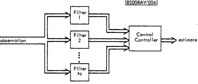
The MMAC method was largely inspired by the work of Magill [8] who

was the first to examine a parallel _{-adaptive estimation algorithm in}

which the basic estimation is done by a bank of filters which are then

coordinated by a centralized controller (see Figure 1.1). Further work

in the area has been done by Lainiotis whose work has been summarized

in [9]. _{The major thrust of this work has been aimed at adaptive}

esti-mation and parameter identification and not the control problem.

Many authors [10, 11, 7] have examined feedback controllers based

on the structure of Magill's estimator, however. For example, Stein

[10]

_{has been able to derive upper and lower bounds on the cost in the} optimal control problem and using the upper bound, has obtained a control

law exhibiting a parallel structure. Saridis and Dao 11] have

ex-ploited Stein's lower bound to obtain a different control law. One

major drawback of both algorithms is that they require significant

on-line computation.

Willner [7] proposed the MMAC algorithm as discussed in this

[85008AW4|I

Filter

observation

2

Jter

Con

tro

Ier

d-5estimate

Filter

-13-upper and lower bounds of Stein. Independently, Deshpande et al [12]

arrived at the same algorithm as an ad hoc extension of the estimation/

identification algorithm of Magill [8]. The method has been further

considered by Lainiotis [13].

To our knowledge, no one has been successful in establishing any

definitive properties on the behavior of the MMAC method.

Specifically,

the convergence properties of the identification problem (i.e., with

the adaptive mechanism disabled) have only recently been proven. Both

Hawkes and Moore [141 and Baram [151 have provided useful results, but

both results do not hold in an adaptive situation (i.e., when the

con-trol law is a function of the system output).

The MMAC method has been applied to various settings. For example,

in Athans et al. [16, 231 the method has been used to control the F-8

aircraft. _{Also, the F-8 controller of Stein et al. [17] can also be}

considered to be a multiple model design. Additional experience with

and insight into the MMAC method has been gained by applying the

esti-mation/identification algorithm to the detection of accidents on

free-ways

18].

To a great extent, the F-8 project 16, 23] has provided the

moti-vation for our work. _{In that project, where the true system does not}

correspond exactly to any of the hypothesized models, several problems

were encountered. First of all, the probabilities often oscillated

rapidly between two models, exhibiting behavior very much like a limit

cycle. This problem led to a design modification consisting of the

A second problem which was encountered involved the choice of which

models to include in the set of possible models.

The aircraft, of course,

responds in a continuous way to parameter changes, and model set selection

was found to have a considerable effect on performance.

It is issues such as these which have motivated our study.

Our

goals have been to understand the characteristics of the MMAC method

and develop a useful design methodology based on the MMAC algorithm.

1.3 Contributions of This Thesis

This thesis presents the results of a detailed study of the MMAC

algorithm.

The major conclusions of this study, which are detailed in

Chapter 6, are of two basic types. First of all, there are specific

conclusions which the analysis of Chapters 4 and 5 yield.

However,

since the analysis of these chapters relies heavily on a special case,

the results are of relatively little direct applicability.

However,

they are indicative of the types of and basic causes for behavior which

has been observed in more general situations.

Thus, of possibly greater

importance are the qualitative conclusions which result when the specific conclusions are extrapolated to general problem structures. These

qualitative results are also detailed in Chapter 6.

The following are the major results of this thesis.

1.

The neutral stability of the MMAC method is established.

2. Conditions which guarantee state convergence are derived.

3. The MMAC algorithm consists of a bank of Kalman Filters,

I I

-15-the system generating -15-the observations (referred to as -15-the true system).

The outputs of each filter are used to calculate the aposteriori

prob-ability that each filter matches the true system. The feedback control

is then given-by the probabilisticly weighted average of the controls

calculated for each hypothesized model. (See Chapter 2 for a complete

discussion). This results in a highly non-linear closed loop system.

However, if the probability is constrained to be constant, then the

closed loop system becomes linear time-invariant. In this thesis it

is shown that even if the closed loop system is unstable for all

constant values of the probability, the overall system may have a

bounded (in fact "hyperbolicly stable" - see Section 4.6) response.

For a special case, specific conditions are derived.

4.

The effects of numerical roundoff are examined and a form of

implementation which behaves well is proposed,

5. The specific results of this thesis can be used to predict the qualitative behavior of MMAC systems which have a more complex structure

than the ones analyzed herein.

4.1 Overview of this Thesis

In Chapter 2, the MMAC algorithm is introduced in the form which

will be used in the reaminder of this thesis. Both the continuous and

discrete time versions of the algorithm are presented, although the

discrete version is employed for the majority of the analysis.

In Chapter 3, the canonical problem which forms the focus for the

situation which retains many of the qualitative properties (such as the

existence of oscillations) which have been observed in more general

problems while simultaneously being amenable to detailed analysis.

The

remainder of the chapter contains a discussion of the various types of

behavior which have been observed in simulations of the canonical problem

along with sample simulation results to illustrate each behavior. The

basic responses are shown to be of three types. In the first, termed

"exponential" or "geometric", the states are geometrically stable.

In

this case, all of the states are decreasing- for all constant values

of the

probability.

The second type termed "oscillatory" results in the

probability

oscillating between zero and one, which in turn results in

the states exhibiting an oscillatory behavior, alternately increasing

and decreasing along with the probability.

The third type termed

"mixed", results in a behavior which, depending on the magnitude of the

initial conditions, exhibits either an oscillatory or exponential

behavior.

These simulations have been used to motivate the analysis

in the remainder of the thesis.

Chapter 4 contains the majority of the analysis of the MMAC method.

In this chapter, each type of behavior described in Chapter 3 is analyzed

in order to yield an understanding of the underlying causes of the

behavior.

This results in conditions which guarantee the existance of

the exponential mode, Furthermore, various approximations are used to characterize the major modes of behavior which lead to conditions for

-17-canonical problem. Beyond this, more general qualitative results are

also presented.

In Chapter 5, various aspects of the problem of implementing the

MMAC method using a digital computer are discussed. By far the most

important of these is the modification to the analysis of the

oscilla-tory behavior when the finite precision nature of the computer becomes

a factor in the behavior. Also discussed are the effects of using

each of the various forms of the equations as far as numerical accuracy

is concerned. The chapter concludes with the proposal of a new form

of the equations which is believed to allow the designer greater latitude

in design without encountering numerical problems.

Chapter 6 contains a discussion of various ad hoc design

modifica-tions which have been proposed in order to overcome the shortcomings of

the MMAC method. Also included there is a summary of the conclusions

of this thesis as well as some suggestions for future research.

1.5 Notation

The following is a brief list of the notation employed in the

thesis. Except for the notation for the components of the residual

of a Kalman Filter, all are believed to be standard.

Mvatrices are represented by upper case letters which are underlined.

Vectors are represented by lower case letters which are underlined.

Scalars are represented by lower case letters (not under-lined).

A' - the transpose of A.

A - _{the norm of a matrix = Max X(A'A)}

X (A) - the set of eigenvalues of a matrix.

N(A) - _{the Null Space of a matrix.}

I

1

-1

xi

-

the

6

-norm of a vector x given by

/'

C1x

for

C51

positive definite.

xjj

- the norm of a vector given by

A U

a - _{magnitude of a real or complex a.}

Ax(k)

-

change

in

x(-)

from k-1 to k.

N

IT

- Product for i=l to N

i=J-N

- Sum for i = 1 to

N

i=1

x

-

vector

of true state variables

X.

- scalar true state component i

(j) .th

r. - scalar 3- component of r. (a,b) - open interval between a and b. [a,b] - _{closed interval between a and b.}

CHAPTER 2

REVIEW OF THE MMAC METHOD

The purpose of the present chapter is to introduce the Multiple

Model Adaptive Control (MMAC) algorithm. A full discussion will not be

given as that is available from other sources

(7,

121.

The MMAC algorithm is composed of two parts. The first, which performs an estimation/identification function, is similar to a Maximum

Aposteriori Probability (MAP) algorithm (151 which is discussed in Section

2.1 for the discrete time case. The MAP algorithm is structured as a bank of Kalman Filters with some decision logic. The second part, which

is cascaded with the MAP-like algorithm, is a control computation 'which

is discussed in Sections 2.2 and 2.3 for the discrete time case.

The remaining sections of this chapter contain a development

and discussion of the special forms of the equations for the MMAC algorithm which prove useful in the remaining chapters of this thesis.

2.1 Maximum Aposteriori Probability (MAP) Identification 2.1.1 The Kalman Filter (KF)

Assume that a linear, time-invariant (LTI) discrete time system is

given by:

x(k+1) = A x(k) +

Bu-lk)

+

C(k)

(2.la)

with observations:

y(k) = Cx

(k)

+ n(k) (2.1b)

-19-

-20-where x(k) is the n-dimensional state vector, u(k) is the m-dimensional

control vector and y(k) is the p-dimensional observation vector. The

noise sources 4(k) and T(k) are taken to be zero mean white Gaussian

noises of covariances E and $ respectively. The matrices A (nxn), B

(nxm), and C (pxn) are the system, input and output matrices respectively. We will use the notation

(A, B, C) (2.2)

to refer to the above system. The system (A, B, C) which generates the

observations y(k) will be called the true system.

In practice, the actual values of the matrices A, B, C, E and

4

are unknown. However, estimates of these parameters are often available from

a knowledge of the system. Thus,, (A. , B. , C. ) will be used to denote th

the i model of the system, given by:

x(k+l) = A.x(k) + B.u(k) +

(k)

(2.3)

y_(k) =

C

x(k) +

n(k)

For the purposes of the present study the values of $ and E will not vary from model to model, although extensions to that case could be

con-sidered.

It is well known that the steady state Kalman Filter (KF) [19, 20]

which estimates the state x(k), based on the model

(A. , B. , C.)

-21-i.

(k+l) = A.W. (k) + B.u(k) +

H.

r. (k+l)

(2.4) r(k+l) =

y(k+l)

- C. [A.i.

(k)

+ B.u(k)]

th

where H. is the Kalman gain for the i- model: -2-.

=

.C

V

(2.5)

and Z. is the nxn solution to the familar Riccati equation

-- t

-1-E=

[Cjt

c.

+

(~A

j

..

+

=)

I

.

(2.6)

The state estimate

i. C)

is n-dimensional, while the residual vector,

-2.

r.

C(-),

is p-dimensional.

2.1.2

Properties of the Kalman Filter

The Kalman Filter has many interesting properties, (see for example

[19]), a few of which are useful in understanding the MMAC method. These

are now discussed.

A few definitions are useful.

Definition 1:

The

th

Kalman

Filter is said to be matched if the matrices

used in the filter design (i.e., the model) and the matrices of the true

system are identical; that is, if A. = A B. = B and C. = C.

Definition 2: The Filter is called mismatched if it is not matched.

th

Property 1:

If the i

Kalman Filter is matched then in steady state:

E{r. (W)1

=

0

(2.7a)

-22-where

6(.)

_{is the impulse function, E{-} denotes expectation, and 6. is}

given by

6

+=4iCE

C,

.(2.7c)

th

Furthermore, if the i filter is matched, then

i^C.()

gives the optimal estimate of the state x().

Property 2: _{If the ith Kalman Filter is matched, then the probability}

density function for the residual r.(-) is given by [20]:

-1

- [5r.'. r]

p(r.)

=

5.e

2

i-(2.8a)

with

=

((2

)m

.

_(2.8b)

Property 3: If the ith Kalman Filter is mismatched then

Ejr. (k)

}

= r. (k) _(2.9a)

-1-t

-Ef(r.

(k) - r. (k))6. (r.

(i)

- r.

(i))

'} =

(k-t)

(2.9b)

where r in general is nonzero and 0. is a function of the system and the

noise covariances (see [28]) with, in general, 0. (0) > I.

It follows that if two filters (one matched and one mismatched) are

computed then

1

-1

E

Ok)e

r

I

())

<

E{r;(k) r2

2(k)}

(2.10)

-23-[16]. _{Thus, if equation (2.8) is evaluated for both a matched (1) and}

a mismatched (2) KF, then

E p(r%)I

>

Efp(r

)}

-

_(2.11)

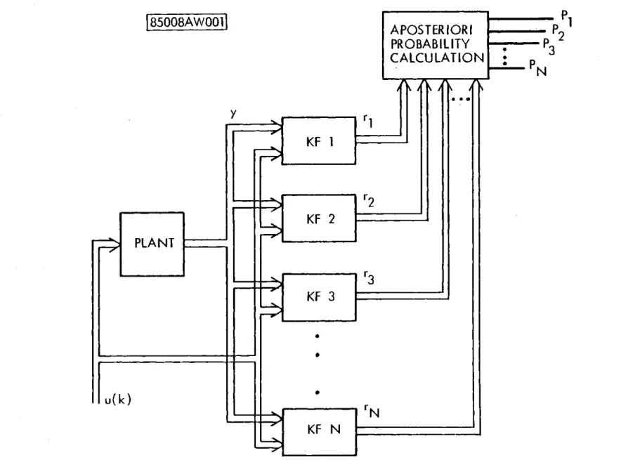
2.1.3 The Probability Equation

Assume that we are interested in identifying a dynamic system from

its outputs and that the true system is known only to be one of N

speci-fied models.

_{Baye's rule and Properties 1-3 imply [15, 7] that the}

th

probability that the i _{model matches the unknown system (P.) is given}

by

P.(k) p(r.(k+l)) P(k+l) =

N.(2.12)

3.N

E

P. (k)p(r. (k+))

j=1

where p (r.(k+l)) is given by equation (2.8). The structure of the

re-sulting system is shown in Figure 2.1.

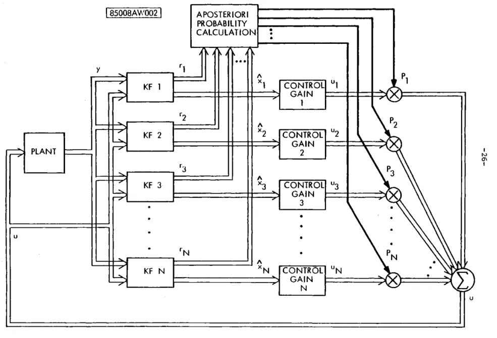
2.2 Adaptive Control

If one knew with certainty which model matched the true system, it

would be a simple matter to design a controller using any of the standard

synthesis techniques. _{Therefore, one reasonable way to determine a} control law for the unknown system is to probabilisticly weight the con-trols _{which would be used if one assumed that one of the models was} correct. That is, let

N

u(k) =

2

P. (k)u. (k) _(2.13)

PLANT

PROBABILITY

CALCULATION

S

N

r3

KF3

r

Ll

KF 3

Fig. 2.1 Identification Structure

"3

-25-where P. (k) is given by equation (2.12) and u. (k) is the control which one would apply if model i were assumed to be matched to the true system.

It will be assumed that

u.

=

G.X."(2.14)

although this is not necessary and is further discussed in Section 2.3.

Figure 2.2 thus summarizes the Multiple Model Adaptive Control method.

2.3 The Control Law

The MMAC method as developed in the literature [7, 16) has assumed

that the linear quadratic (LQ) methodology is used to design the controller.

Thus, the feedback gains G. of equation (2.14) are chosen to minimize

-J(u)

=

2 (x'(k)Ox(k)

+

u' (k)R

u

(k))

.

(2.15)

k=J

It can be shown [211 that the optimal gains are given by

G. = [B!K.B. + RI

1

B'K.A.

(2.16)

where K. is the solution to the steady state Riccati equation

K.

=

Q.

+ A'K.A. - A!K..B, [B!K.B. + RI B..K,A.

(2.17)

Although to date, all references to MMAC have made use of the control

law (2.16), this is not a necessary part of the method. Thus, any control

law which gives good results for the respective model may be used.

How-ever, there is a strong interaction between control law choice and

PLANT

U1

PROBABILITY

CALCULATION

y

r

KF 1I1

r2A

KF 2

2N

-

3-x

r3N

KF N

xN

P1

CONTROL

u2

G AIN

P

u2

CONTROL

2

GAIN

2

₁

3

CONTROL

u3

GAIN

x

31

N

[CONTROL

N

GA N

Fig. 2.2 Adaptive Control Structure

For the purposes of this study we will for the most part restrict our

research to control laws based on the linear quadratic (Equation 2.15)

form.

2.4 Comments on MMAC

A few comments are in order.

1)

The MMAC algorithm, as shown by Willner

f7]

is suboptimal even

for the problem originally posed. Willner was able to show that the

algorithm is optimal for the final step of the dynamic programming algorithm [7] but was unable to continue the calculation backward in time.

2) As posed above, the true model is assumed to belong to a finite set of known models. Lainiotis

[9,

13] has discussed the infinite set case but concludes that a finite approximation is then required for use

in applications. Thus, for most real problems when the true model may

take values from an infinite set, a further suboptimal approximation is

required.

The results of Baram

[15]

(which. apply only to the open-loop

case) may help in discretizing the model set.

2.5 Continuous Time MMAC

As. developed in the preceeding sections, the MMAC method has been based on discrete time systems. For analysis purposes, it will be useful

to consider the related continuous time problem, largely because of the

simplified form of the probability equation.

The complete equations for the method will not be given here. as they are the continuous time regulator and continuous time Kalman Filter

Dunn [22] has shown that if P. (t) is the probability of the it model at time t then

N N

-.

-K1

P.

_1.

Ct)

=

P.

₁

(C.i.

-

E

P.C.SU)G

(y -(P.C.2.)

(2.18)

1-1=r

-3-3

j=lJ3

where C.,

x.

and y are defined analogously to

the discrete time case and

6 is the observation noise covariance.

The property which makes Equation

(2.18) useful for analysis is the absence of either exponentials or a

denominator.

These equations are examined further in the two model, two

state case in the following section.

2.6 A Special Case

Of special interest to the (i.e., the two model case) with shall assume that the input (B)

The special case capturesa

we are interested in examining A

it forms the central focus for t

research at hand is the case when N=2

full state observation.

Furthermore,

we

matrix is the identity.

all essential features of the problem that

without adding unnecessary complexity, and

this research.

2.6.1 Discrete Time Case

In the discrete time case, the true system is then given by

x(k+l)

=

Ax

(k) + u(k) + ;_(k)

(2.

19a)

yk)

=

x(k)

+ _(k)

with models

Model

1:

i

(k+l) = A R (k) + u(k) +

C

c)

-1

-1--1-y(k)

=

2

(kc)

+

r~k)

-_ -l -_ (2. 19b)

-29-Model

2:

2^

(k+l)

=

A

i(2k>

+

uk)

+

C2k

-2

_(2

-2-2

.l9c)

y (k) = 2(k) +

r(k).

Thus, the MMAC method reduces to the following set of discrete time

equations

x

(k+l) =

Ax

(k) + u(k) +

C

(k) y(k) =

x(k)

+

c(k)

(k+l) =

A2

(k) + u(k) +

H r

(k+l) (k+l) =y(k+l) -A k) - u (k)

2

(k+1) =

A2

(k) +

u(k)

+ H r (k+l) (2.20)

-2z-2-2

2-E2

2 (k+l) = y (k+1) -

A2

(Ik)

-

u(k)

u (k)

=

-Pc2

(k)

-

P2

c2

(k)

-

11-12-2z-2

P (k) p(

P

(k+l) ₁

1

P

1

(k)

p

(r

1

)

+

P

2

(k)

p

(

2

)

-

fr.1

r.

P(r )

fSe

The major goal of the research has been to understand such qualitative

properties of the MMAC method as stability. Since the phenomenon which

have been observed are largely due to the nonlinearities of the system

and occur even in noise-free simulations, the noise terms

C(-)

and T(.) add an unnecessary complexity. Thus, these terms are ignored in the

assuming the noises to be present, are. an integral part of the MMAC method and are therefore retained. Thus, the principle focus of the work is to examine the deterministic properties of Equation (2.20) and the correspond-ing continuous time system discussed in the next subsection. Since the

sum of the probabilities of the models

must

always be 1, it

is known that

P2(k) = (1-P 1(k))

Vk.

Then, rewriting Equation (2.20) in terms of the residual r (k) we see

that the equations of the MMAC method can be summarized by

x(k+l) = Ax

(k)

+ uk)

r (k+1) = (A-A )x(k) + A

(I-H

)r

(k)

E2 (k+l) = (A-A2)x(k) + A(--2

)r(k)

(2.21)

--2

-(-2--21-u(k)

=

-(P G

+ (1-P)

G

-(k) + P

G (I-H r

+

Cl-P G

(I-H

)r

S1-11

-2--t

- -2

-2-2

P

1

Ck) p(r

1

)

P (k+)

P1=

1(

P(k) p() + (1-P (k))p

1

-l

1

-1

-1

- - [r6 r.) p(r.) =

S.e

It will be useful notationally to combine the state and residual

equations into one vector equation. Therefore, we define the vector

w

(k) = [x (k), r'C(k) , r'2(k)]' .

-31-A-PG

-

C-P)G

PG(I-H)C(1-P)G (I-H)

-a, - U 1)-2 :1-1 -- : 1) -2 I -- 2 (2.22b) ... a... ... w(k+(A-A) A(I-H)

0

w(k)

...

...

...

(A-A) _{0 -2 A(-2} or w(k+l) = i(P )w(k) with

P

(k)p~

P (k+1)= (2.22b)

1(Pk(k))p(=)

) + (1-P(k))p(r2)

These equations, along with their continuous time counterparts, form the

basis for the research which has been undertaken.

2.6.2 Continuous Time Case

Similar assumptions to those previously presented for the discrete

time case can be made in the continuous time case. Here, we will again restrict our attention to the two model, state feedback case with B=I. Thus, the MMAC method reduces to the following equations

iC(t)

= Ax (t) + u(t) + C(t) y(t) = r(t) + 1(t)

E

(t)

= A 2(t)

+ u(.t) + HrWCt)

(2.23)

r (t) = y(t) - x (t)

-1

-

-1

2(t) = A 2 (t) + uCt) +

H

2(t)

-2

-2-z2--r2t)

= y(t) - ^2(t)

1-2

-2

u

t)

= -P1G ( t) - P

t)

1 iz-

2 -22 2*2 (

1

p(t)=

P1 (t)

P2(t)Ii

1

(t)-i (t)J'

[x-P1 (t)i-(-PC1

(t)

)2

Ct)

]

with P2 (t) = 1-P1(t).

For the

same

reasons as presented in the previous section the noise

sources _(t) and _(t) will again be ignored for the majority of the

proposed research. It should be noted that under this condition, the

residual r.(t) exactly equals the estimation error x(t) - x.(t). Thus,

equations (2.23) can be rewritten as

5(t)

=

Ax

(t) + u(t) (t) =A -H )r(t) + (A-A )x(t) (2.24) L2(t) = (A-H )r2(t) + (A-A )x(t)

-2:-2

z-2 :-2

--- 2

u(t) = -P (t)G

(x(t)

-

(t))

- (1-P (t))

G

(x(t) - r (t)) - 1

-1-

-11

--

2

P (t) = P1(t) El-P1(t)] Er2(t) -

1(t)]'

0

1

EP

(t)

1(t)

+ (1-P (t))r (t)]

Thus, if we again combine equations by defining the variable

x(t)

w(t)= r(t)

r (t) E2 -2t(r

-33-PGA

-

Cl-p

(A - 2

(A-A)"AH

1=2--1

12

0

-2

2

w

(t)

(2.25a)

or

with.

w(t)

_--

= A-P,

i(P )w~t)

-(-,

(2.

25b)

-K'

P Ct)

=

P

(t) [1-P (t)1)r2(t) -

r

(t)]

[p

(t)r (t) + (1-P(t))r2(t)] 1

1=1-2

-1

-l1

"z-2

2.7

A Change of Variable

A change of variable which proves useful in the sequel is to let

(2.26)

q = 2P1 -1

Making this change in Equation (2.22) yields

w(k+1) =

A(q)

w(k)

(1+q)p(Er)

-

(1-q)p(r

₂

(l+q)p(r

1

)

+

(1-q) p

(r

2

where

(2.27)

1

1

A_--L

A -A2

I'

(1+q)G

(-)

- )

In continuous time the corresponding change to Equation (2.25) yields

EA

w'(t) =

_(q) =

(A-q)

where

w(t)

=

(q)

w

(t)

4t(t)

= -(-q2

)r-r'6

(l+q)r

1 +

(1-q)r

2

]

1

1

..

A- (+q)G

₁

-

(.l-q).G

₂

j.(l+q-)G

2 2 (q)=

(2.28)

--

2.-.A-

2

Note that the same basic notation is used for the A matrices of Equations (2.22), (2.25), (2.27) and (2.28). However', no confusion should arise as the meaning should always be clear from context.

2.8 A Useful Definition

A further concept which will prove useful can be seen by considering either the continuous or discrete time problems as summarized by either Equation (2.25) or (2.22)

Continuous

time:

w

(t)

= Ai(

)w(t)

-t

-

1

-Discrete time:

w(k+l)

=

A(P )w(k)

-

-l-

(2.25)-(2.22)

where

Continous time:

Discrete

time.;

A-.PG -a,-a1-p

_1-1

1)G2

_1-2

A A A- A - -2 A- A

A- A

--- 2

A-

' -0 A) (aH P12 AIH) (-H - -- 2 -)2(

-35-Thus, it is clear that if P

(-)

is held constant, then Equations (2.25)

and (2.22) describe linear, time-invariant dynamical systems in the

variable w' = [x', r', r']'. Thus, Equations (2.25) and (2.22) with

- - -1 -2

P constant will be referred to as the linear, time invariant system for fixed P, or LTI for fixed P. As will be seen in Chapters 4 and 5, many of the major properties of the MMAC method can be expressed in terms of

the properties of the LTI system for fixed P as a function of P. A second important point to note is that in applications and simulations of the MMAC system, another parameter becomes important due to the finite precision usually available for computation. From the equations of this chapter, it is clear that the MMAC method has the

property that

P. (k) 0= -P. C-) = 0 for all future times.

1 1

Such a situation is usually to be avoided, as it

reduces the flexibility

of the algorithm in a number of applications.

For example, the parameter

of the true model are often changing in adaptive control situations, and one would like to require P. to be nonzero for all time so that the MMAC algorithm can respond to such changes. Thus, one almost always: applies

an additional constraint on the probability such as

P. Ck)

>

P

.

i

, k.

1 - .lim

-50

This has been done throughout this study with a value of Plim =10 The effect of such a limit is examined in detail in Section 5.1.

QUALITATIVE RESULTS

In order to guide and motivate the research, we have examined a problem consisting of a system with two independent states and two models.

This

system, while simple, captures many of the basic issues which are

important to the method and sheds light on the fundamental problems

in-volved with the MMAC design. The problem is formulated in the next

section of this chapter. The remaining sections contain simulations

which demonstrate the various types of behavior which have been observed.

A discussion of the important properties is included.

3.1 Problem Formulation

In most applications, of an adaptive control algorithm, a detailed

analysis of the behavior of the algorithm has proved intractable. This

is especially true for the MMAC algorithm.

However, in the case of

MMAC,

it

is possible to find a simple example problem that lends itself

to analysis and simultaneously maintains the basic properties exhibited

in simulations of the more general systems.

Thus, for the purposes of

this thesis, a sample problem structure has been chosen which displays

what we feel are the critical characteristics of the method and which

is also amenable to detailed analysis.

The chosen true system to be controlled is given by:

a 0

x_(k+1) = x (k) + u(k) +

rVk)

(3.1)

0

a

L (k) =x (k) + -n.k)

-36-

-37-or a continuous time system of the same structure and A matrix

a

0

(t) =

[

]x(t)

+

u(t)

+ (t)

Lt

a

y_(t) = (t) + TI(t)

where a takes on values in the range [0,

21.

The discrete

is useful for simulation studies and most of the analysis.

of the continuous time system provides greater insight for

tion results in Section 4.1.

The set of models for either

or continuous time case is given by

Model

1:

(A,1, I) Model 2: (A,2 , I)

with

time system

However, use the lineariza-the discrete A

0

:i

A2

:i

where

i

takes on various values from 0 to 1.5.

The parameters a and

i

are varied to obtain different responses from the overall system.

For the purposes of

KF

design, the noise sources

(-) and n(-) are

assumed to be zero mean, white and Gaussian with covariances of I&(-)

where I is the 2x2 identity matrix.

This structure results in diagonal

Kalman Gain matrices such that

h

0

LO

h

(3.2)

I I

h

0

LO

hj

's

where h is the gain corresponding to a and h is the gain corresponding

to

a.

Further, the control law weight

and R, are chosen diagonal such

that

R R =I

-l

-2

-q 0 q

0-21=11

:i22[

.]

[ qI 0 q_

This results in a diagonal control gain matrix

g9 0 J

0-G =G =.

0 g 0 g

The structure described above

will

be referred to as the canonical problem.

The emphasis of this study has been on the examination of such

quali-tative properties as stability.

Thus, we ignore the noise sources both

in the simulation and in the analysis of the properties of the MMAC

method.

That is, in both the analysis and simulations, C(-) and Tr(-)

are

set equal to zero. Note, however, that the

KF's

designed with the assumed non-zero noise sources are retained. It is clear that noise can have

a major effect on a system [29].

However, as we will see, many of the

properties of the MMAC method are due to the nonlinearities of the

probability equation.

Thus, it

is our feeling that an anlysis of this

noise-free case is of considerable importance.

A few comments are in order concerning the the choice of the example problem. First of all, the system is chosen to be the simplest possible

.I I

-39-state, two model system. The choice of model is, admittedly, somewhat

extreme in the degree of symmetry and mismatch between the models and

the true system. _{However, this choice has been deliberately made in order}

to investigate phenomena which have been observed in actual applications

123].

_{Thus, it is felt that the analysis of this problem has yielded}

insight into the more general case.

3.2 Basic Responses

Various types of responses have been observed in simulations of the

system presented in Section 3.1. Table 3.1 details the parameters used

for each simulation. _{The remainder of this chapter presents examples}

of each of the major modes along with a discussion of the important

characteristics of each. The simulations, which have been performed on

an IBM 370 computer using double precision FORTRAN, have been used to

motivate and guide the analysis of Chapters 4 and 5.

In fact, the types

of analysis described in these chapters and, in particular in Section

4.6, were to a large degree suggested by the simulations discussed in

this chapter.

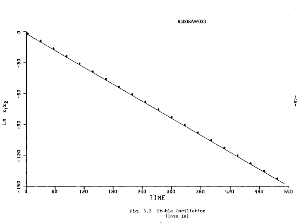
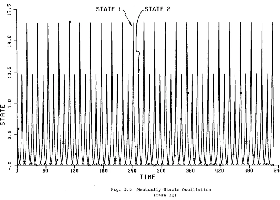
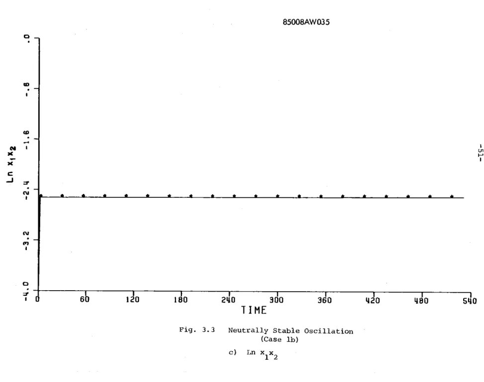
For each simulation presented, three plots have been included. The

first is a plot of the probability of model one (P1) versus time. The

second is a plot of the two true states x1 and x2 versus time. The third

is a plot of the quantity ln(x₁x2). This quantity has been found to be

indicative of the stability of the closed loop, nonlinear system. This

variable is further discussed in Section 4.6 where it is linked with

Case

#

la

lb

lc

2

3

a

a

2 2

2

1.5

.9

0

0

0

1.0

0

q

g

g

h

Ii

Figures

1.02

0--*

1

1

1.62

1.5

1.4

1.09

.538

1

1

1

1

1

0

0

0

.618

0

.809

.809

.809

.7245

.597

.5

.5

.5

.62

.5

TABLE 3.1

Parameters of Sample Cases

*This value of the control can not result from an LQ design. 3.2

3.3

3.4

3.5,6

3.1

I I .

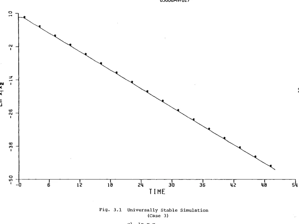
-41-3.2.1 Exponential Mode

The first type of behavior is one in which the states of the true

system increase or decrease in an exponential manner (see Figure 3.1).

This type of behavior appears to arise in two situations. First,

examination of the equations of Chapter 2 indicate that if the KF

resi-duals r1and r2 are equal with the true state components equal to each

other, then P t) = 0 or equivalently, PC(k+l) = P (k). Thus, if the system is symmetrically initialized (that is, the two true states are

equal with

rl

=

r2

=

0

and P1 (0) = .5) then P1(t) = .5

Vt

or equivalently P (k) = .5 V k. The closed loop system is then time invariant and sta-bility analysis for the resulting LTI system follows as usual. Note that

the resulting system can be exponentially stable, neutrally stable or

exponentially unstable depending on the control gains G and G .

Al--l

-2

though this is clearly a singular condition, it nonetheless is important

from an applications point of view because one commonly attempts to

initialize the system with equal probability and with rl = r2 (i.e., x 2=). An analysis of this mode is presented in Section 4.1.

A somewhat similar type of behavior occurs when the LTI system for fixed P is stable for all P. This, of course, is a fairly restrictive

condition which in essence requires extreme robustness of each controller.

However, such a condition does imply exponential stability. This occurs

in-dependently of how the probability behaves. Note that this is a

non-trivial result since A(P(k)) is time-varying because P(k) is. Section

4.2 contains the analysis of this situation and Figure 3.1 is an example

is

24

30

T I ME

Fig. 3.1 Universally Stable Simulation (Case 3) a) Probability of Model 1

36

0 M~ 0 CE)

-J

LUI

C

F-cc

C

. C: CU 0 M

'Li

-o

6

12

42

48

SI4

I 69t) .fir & 46 46 Aw 46

85008AW026

M

-

STATE I

cr-

STATE 2

(n -06 12 18 24 30 36 42 48

Fig. 3.1 Universally Stable Simulation (Case 3)

M

('A

I x CD (i

-06

12

18

24

30

36

42

48

Fig. 3.1 Universally Stable Simulation (Case 3)

-45-3.2.2 Oscillatory Reponse

Probably the most unusual behavior which has been observed both in

the current work and in applications of the MMAC algorithm (23] has been

an oscillatory response in which the probability jumps between

near-zero and near-one* in what appears to be (but strictly speaking is not)

a limit cycle.

Figures 3.2 through 3.4 are examples of this type of behavior.

Figure

3.2 is a case in which the

peaks

of the state trajectories are

approxi-mately constant while the period of oscillation increases.

Figure 3.3

is a case in which both the peaks and the period are constant while in

Figure 3.4, the system is unstable,

These three cases are obtainad by

changing the value of the control gain. Note that each gain would yield

stable behavior for the model used in its design.

It is interesting to note that the states of the system are also

highly oscillatory,

It might be expected that the plant dynamics would

smooth the rapid probability transitions to form a smoother "average"

state response. However, as shown in Chapter 4, the oscillatory state

behavior is a direct consequence of the model mismatch problem in the

MMAC algorithm.

The reasons for this oscillatory behavior, which are discussed in

Sections 4.4 through 4.6 and again in Section 5.1, are closely related

to the fact that neither of the hypothesized models individually yields

*This is the one set of simulations in which the lower limit on the probability (.see Section 2.8) of 10-50 is achieved. Section 5.1 dis-cusses the analysis in this case in detail.

-

~

-

.

.L 4 W'- --- d,---4 - iA - I ____1______________ 6

240

TI

ME

300

360

Fig. 3.2 Stable Oscillation (Case

la)

a)

Probability of Model 1

0 0 0D OL _{t *} -i

Lui

0

CC

L I:)

cc:

CL

0 CD-0 flu-0 (V 0

I

60

180

₄₂₀

₄₈₀

₅₄₀

* I& dr AL-46 .A6

Ah-120

85008AW032

STATE 1

akr i

IWSTATE

.2

% . vaa- %,a I& M.- -

J

-~ -~ -~ _~1 - :r.--:~ -- 1 -.I ~ -- - -I- -~- I

240

300

360

TI ME

Fig. 3.2 Stable Oscillation (Case

la)

b) True States

Ln

0

LLu

F

-09

In

04

0

A

U

V

A

it

Y

41

60

120

2

180

420

ka

480

540

WA

C O ('1-V 0 60 120 180 240 300 360 420 480 540

T I

M

E

Fig. 3,2 Stable oscillation

(Case la)

c)

85008AW034

0 Cc

CL

rC

-b~

0.

ILUL II U J-LLH ALI HILI-4L 1. J11.1 JI III

360

Ai

4 1 I

420

480

S54O

Fig. 3.3 Neutrally Stable Oscillation (Case lb) a) Probability of Model 1

r-4

HHn

I I I

300

T

I

M E

I0

663

120

180

240

STATE

I

STATE 2

t

-I-. -- -- -~

V

240

30

360

TI

M E

Fig. 3.3 Neutrally Stable Oscillation (Case lb)

b)

True States

0 Lfl 0 0

LuI

F-a:

F-WI

0

0

60

120

180

0

iLID

420

'iao

W

C4U'l

I

85008AW035

H a A * a * * * * a A a.6 * a a A

300

T I M E

Fig. 3.3 Neutrally Stable (Case lb)

c)

Ln

x12

Oscillation

09-0 31C CD I CV C'? 0

-r

[

60

120

180

240

360

420

480

540

0 C3 C . ED0 .

ED

TEIw

C(%J

Fig. 3.4 Unstable Oscillation

(Case 1-c)