Automated Understanding of Data Visualizations
by
Sami Thabet Alsheikh
S.B., Massachusetts Institute of Technology (2016)
Submitted to the Department of Electrical Engineering and Computer
Science
in partial fulfillment of the requirements for the degree of
Master of Engineering in Electrical Engineering and Computer Science
at the
MASSACHUSETTS INSTITUTE OF TECHNOLOGY
June 2017
c
○ Massachusetts Institute of Technology 2017. All rights reserved.
Author . . . .
Department of Electrical Engineering and Computer Science
May 12, 2017
Certified by . . . .
Frédo Durand
Professor
Thesis Supervisor
Accepted by . . . .
Christopher J. Terman
Chairman, Masters of Engineering Thesis Committee
Automated Understanding of Data Visualizations
by
Sami Thabet Alsheikh
Submitted to the Department of Electrical Engineering and Computer Science on May 12, 2017, in partial fulfillment of the
requirements for the degree of
Master of Engineering in Electrical Engineering and Computer Science
Abstract
When a person views a data visualization (graph, chart, infographic, etc.), they read the text and process the images to quickly understand the communicated message. This research works toward emulating this ability in computers. In pursuing this goal, we have explored three primary research objectives: 1) extracting and ranking the most relevant keywords in a data visualization 2) predicting a sensible topic and multiple subtopics for a data vi-sualization, and 3) extracting relevant pictographs from a data visualization. For the first task, we create an automatic text extraction and ranking system which we evaluate on 202 MASSVIS data visualizations. For the last two objectives, we curate a more diverse and complex dataset, Visually. We devise a computational approach that automatically outputs textual and visual elements predicted representative of the data visualization content. Con-cretely, from the curated Visually dataset of 29K large infographic images sampled across 26 categories and 391 tags, we present an automated two step approach: first, we use ex-tracted text to predict the text tags indicative of the infographic content, and second, we use these predicted text tags to localize the most diagnostic visual elements (what we have called “visual tags"). We report performances on a categorization and multi-label tag pre-diction problem and compare the results to human annotations. Our results show promise for automated human-like understanding of data visualizations.
Thesis Supervisor: Frédo Durand Title: Professor
Acknowledgments
I would like to thank
∙ Zoya Bylinskii, who has been an great friend and even greater mentor.
∙ Spandan Madan, Adriá Recasens, and Kimberli Zhong, without whom this research would not have been possible.
∙ Frédo Durand, who has been a very supportive and trusting adviser.
∙ Aude Oliva, who has been a steady source of encouragement and enthusiasm. ∙ My family and friends from Boston, Pensacola, and Syria, who have made me the
person I am.
Finally, I would like to thank my parents, Thabet Alsheikh and Omaima Mousa, and my three siblings, Kinan, Dima, and Nora, for being constant reminders of what matters most.
Contents
1 Introduction 13
1.1 Overview . . . 13
2 Background 17 2.1 What are data visualizations? . . . 17
2.2 Neural networks . . . 18
2.3 Datasets for data visualizations . . . 19
2.3.1 MASSVIS . . . 19
2.3.2 Visually . . . 19
2.4 Related work . . . 21
3 Visually important text extraction 23 3.1 Problem . . . 23 3.2 Approach . . . 24 3.2.1 Data collection . . . 24 3.2.2 Text extraction . . . 24 3.2.3 Ranking . . . 27 3.3 Results . . . 27
4 Category and tag prediction 31 4.1 Problem . . . 31
4.2 Approach . . . 31
4.2.2 Image patches to labels . . . 34 4.2.3 Technical details . . . 35 4.3 Results . . . 36 4.3.1 Category prediction . . . 36 4.3.2 Tag prediction . . . 37 4.4 User study . . . 41 4.4.1 Data collection . . . 41
4.4.2 Evaluating the text tags . . . 42
5 Visual tag discovery 43 5.1 Problem . . . 43
5.2 Approach . . . 44
5.3 Results & user study . . . 45
5.3.1 Data collection . . . 45
5.3.2 Evaluating the visual model activations . . . 47
5.3.3 Evaluating the extracted visual tags . . . 48
6 Conclusion 51 6.1 Contributions and discussion . . . 51
6.2 Looking forward . . . 52
A Visually dataset 55 B Category and tag prediction supplemental material 59 B.1 Additional baselines . . . 59
List of Figures
1-1 Examples of data visualizations . . . 14
1-2 An overview of our system for extracting and ranking text . . . 14
1-3 An overview of our system for predicting text and visual tags . . . 15
2-1 Sample data visualizations from the MASSVIS dataset . . . 19
2-2 Sample infographics from the Visually dataset . . . 20
3-1 A motivating example for ranked text extraction . . . 23
3-2 An input, ground-truth map, and output for the Visual Importance Predictor 25 3-3 An example input and output from the Oxford Text Spotter . . . 25
3-4 Our augmented Text Spotter which consolidates multi-scale results . . . 26
3-5 Results for querying “Japan" in our ranked text extraction system . . . 28
4-1 An example infographic of a soccer player with its category and tags . . . . 32
4-2 Our proposed training procedures for category/tag prediction. . . 33
4-3 The top activating patches per category for all 26 Visually categories . . . . 38
4-4 Examples of how text and visual features can work together in tag prediction 41 4-5 Task used to gather human annotations for text tags . . . 42
5-1 Visual network activations for different categories on one infographic . . . 44
5-2 Samples of visual tags extracted for different concepts. . . 45
5-3 Automatic text and visual tag prediction examples . . . 46
5-4 Task used to gather human annotations for visual tags . . . 47
6-1 Natural image research that could apply to data visualizations . . . 53
A-1 Visually dataset size vs. number of included tags . . . 56
A-2 Histogram of image sizes in the Visually dataset . . . 56
B-1 Confusion matrix for category predicted by textual features . . . 61
List of Tables
2.1 Visuallydataset statistics before and after cleaning . . . 20
3.1 The mean AP results for ranked text extraction methods . . . 28
4.1 Results on category prediction . . . 37
4.2 Results on tag prediction . . . 40
5.1 Visual tagging class-conditional evaluations . . . 48
A.1 Manually removed tags from Visually . . . 57
A.2 Manually determined tag mappings for Visually . . . 57
A.3 The final set of 391 tags for our text and visual tagging problem. . . 58
Chapter 1
Introduction
Whether it is in school, business meetings, or the media, humans are often presented with graphs, charts, infographics, and other data visualizations. To a computer, these visual-izations are simply grids of pixel values. To a person, the same visualvisual-izations are media intended to communicate a message. The computer vision research community has created systems able to understand and caption images of natural scenes, like a photo of a boy play-ing tennis [13]. However, to our knowledge, there has been little work focused on creatplay-ing this understanding in the context of data visualizations.
When a person views a data visualization like the ones shown in Figure 1-1, they read the text and process the images to quickly understand the overarching story. This research works toward emulating this ability in computers.
In pursuing this goal, we have explored three primary research objectives: 1) extracting and ranking the most relevant words in a data visualization 2) assigning a sensible topic and multiple subtopic tags to a data visualization, and 3) extracting relevant pictographs from a data visualization.
1.1
Overview
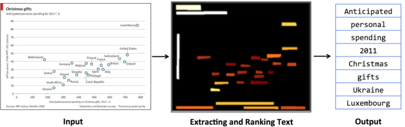
To gain context from a data visualization, a human will often rely on the image’s words. Noting this tendency, we first focus on extracting and identifying the keywords in these images. Our ranked text extraction system can be seen in Figure 1-2.
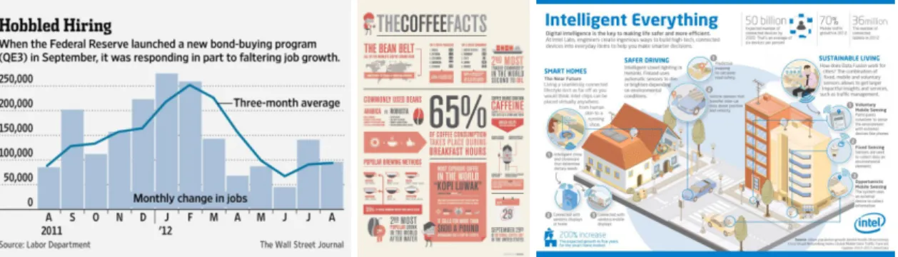
Figure 1-1: Examples of data visualizations. The middle and right images are special types of data visualizations called infographics (data visualizations that contain pictorial elements). Sources: MASSVIS [6] and Visually Datasets.
Figure 1-2: An overview of our system which ranks by importance the text in any visual-ization. The text is spotted and extracted, then ranked by an importance map.
After extracting and ranking the text embedded in a data visualization, we explore ways to assign relevant text topics and tags not necessarily found inside the image. More specif-ically, we build a data-driven system that can predict one of 26 categories (topic) and a few of 391 tags (subtopics) given an infographic. We explore predictions that leverage both extracted text and visual features.
After developing the category/tag prediction system, we find that text extracted from within the infographic is a better topic predictor. We explore whether this extracted text can guide our visual system. We introduce the problem of visual tag discovery: extracting iconic images that represent key topics of an infographic. An example of our system that can assign tags and extract visual tags can be seen in Figure 1-3.
The systems developed through this research work toward general visualization under-standing, but the work also provides some immediate application areas. For example, rank-ing extracted text or assignrank-ing relevant topics can be leveraged for smarter visualization tagging to be used in online search. Additionally, our visual tags can provide nice picture summaries for concise communication and sharing on social media. Although these
imme-diate application areas exist, we are more motivated by advancing the space of visualization understanding.
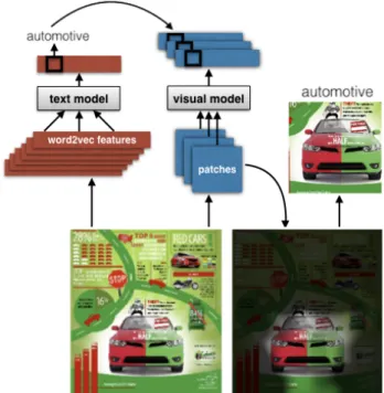
Figure 1-3: An overview of our system for predicting text and visual tags. The text in an infographic predicts the tags, the visual model fires on the patches that most activate for this tag, and a segmentation pipeline is run to extract the representative visual elements from the highly activating regions of the infographic. The result is automatically generated by our model.
Chapter 2
Background
In this chapter, we first explain this research’s domain (data visualizations) and primary tool (neural networks). Because our system heavily relies on data-driven neural networks, it is also important to understand the datasets we use. Last, we survey related work.
2.1
What are data visualizations?
Data visualizations are visual representations of data (numerical and otherwise) created to help communicate a message. This definition seems very inclusive because the concept itself is inclusive! Some examples of data visualizations can be seen in Figure 1-1. Note the wide variety of styles, designs, and information that can be used: data visualizations can range from simple pie charts to complicated storyboards. A subset of data visualiza-tions that we focus on in this research are infographics. Infographics are a type of data visualization that rely on both visual and textual elements to communicate a message.
With growing amounts of data, navigating and visualizing large datasets to highlight meaningful trends has become of great interest. For our purposes, we are interested in the fact that these messages are often complex and require higher-level cognition to process.
2.2
Neural networks
Neural networks are computational models that can approximate complex, non-linear func-tions. They are often used in machine learning to create a system that can approximate how inputs map to outputs for a given task. For example, in computer vision, neural networks might be used to approximate how the input pixels of an image map to a label for that image, like a scene category or topic. In between the input and output layers, there are often many hidden layers. Each of these layers are composed of many “neurons," which have their own activation functions to process inputs and produce outputs. In feedforward networks, the outputs from each of these nodes in a given layer will feed into the inputs of the subsequent layers after being multiplied by tunable weights.
This powerful representation allows neural networks to approximate very complex functions. In practice, these neural networks will have many layers, making them deep neural networks. The model’s weights can be trained on a large set of input-output pairs to then predict outputs on new inputs. In the case of this research, we often have many data visualizations with a topic label (e.g. sports), and if we later see similar data visualizations for which we do not have a label, we hope that the network will be able to identify that the new input is about sports. Neural networks with a convolutional layer are particularly suited for working with images, due to having fewer parameters to train. Their recent success is also attributed to larger curated datasets to learn from and better hardware to train on. As a result, they have gained popularity in the computer vision community, and have shown top performances on scene recognition, object detection, and other image understanding tasks [27].
Recently, a particular kind of convolutional neural network, residual networks (ResNet), have proven to be one of the most successful architectures for image classification [11]. These networks include “shortcut connections" which connect every other layer not only to the next layer, but also the layer after the next layer. The inventors show these networks achieve state-of-the-art results for image classification, are easier to train, and can have many more layers in practice. Because of this success, one of our systems is directly built on top of ResNet. For a detailed account of deep neural networks, we refer the reader to
Figure 2-1: Sample data visualizations from the MASSVIS dataset. Note that the dataset in-cludes more basic charts and graphs to data visualizations to those that have more complex features.
Goodfellow et al.’s book, Deep Learning [9].
2.3
Datasets for data visualizations
Because this research uses a machine learning approach, the datasets we use heavily influ-ence the power of our system. We leverage two datasets: MASSVIS and Visually.
2.3.1
MASSVIS
For ranked text extraction, we use the Massachusetts (Massive) Visualization Dataset (MASSVIS) [6]. MASSVIS includes 5k images of data visualizations obtained from various sources in-cluding government, news media, and scientific publications.
Since the initial dataset release, the curators have collected human clicks and captions on these visualizations, allowing us to train our system and evaluate the results, respectively [7]. For an account of this dataset’s creation, please refer to [6] and the MASSVIS website.
2.3.2
Visually
For the rest of the research, we seek to address more complex image-understanding tasks, which requires a larger scale dataset. We curate and use the Visually dataset (http://visual.ly/view) which includes 29k large infographics.
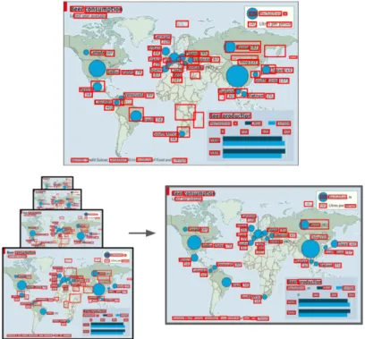
We scraped 63,885 infographic images from the Visually website, a community plat-form for hand-curated visual content. Each infographic is hand categorized, tagged, and
(a) (b)
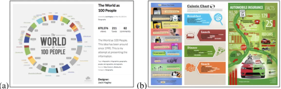
Figure 2-2: (a) Sample data available from Visually. We scraped over 63K infographics containing category, tags, and other annotations. (b) A few infographics from the dataset demonstrating the mix of textual and visual regions, the richness of visual content, and styles.
described by the designer, making it a rich source of annotated images. Despite the dif-ference in visual content, compared to other scene text datasets such as ICDAR 03 [19], ICDAR 15 [16], COCO-Text [28] and VGG SynthText in the wild [10], the Visually dataset is similar in size and richness of text annotations, with metadata including labels for 26 cat-egories (available for 90.21% of the images), 19K tags (for 76.81% of the images), titles (99.98%) and descriptions (93.82%). Viewer likes, comments, and shares were also col-lected. For a subset of 1193 images, full transcripts are available.
Dataset # of categ. Images per category # of tags Images per tag Tags per Image 63k (full) 26 min=184 max=9481 mean=2235 19,469 min=1 max=3784 mean=7.8 min=0 max=10 mean=3.7 29k (clean) 26 min=118 max=4469 mean=1114 391 min=50 max=2331 mean=151 min=1 max=9 mean=2.1
Table 2.1: Visually dataset statistics. We curated the original 63K infographics available on Visually to produce a representative dataset with consistent tags and sufficient instances per tag.
We curated a subset of this 63K dataset to obtain a representative subset of 28,977 images (Table 2.1). Uploaded tags are free text, so many of the original tags are either semantically redundant or have too few instances. Redundant tags were merged using WordNet and manually, and only the 391 tags with at least 50 image instances each were retained. To produce the final 29K dataset, we further filtered images to contain a category
annotation, at least one of the 391 tags, and a visual aspect ratio between 1:5 and 5:1. Of this dataset, 10% was held out as our test set, and the rest of the 26K images were used for training our text and visual models. For 330 of the test images, we collected additional crowd-sourced textual tags and visual element bounding boxes for finer-grained evaluation. For a full account of the dataset creation and more statistics, please refer to Appendix A.
2.4
Related work
Diagram understanding: While the computer vision community has made lots of progress with models able to localize meaningful objects and describe the visual content of natural images, digitally born media has received little attention. Most of the work that has been done on non-natural images has been in diagram understanding. For example, [26] focuses on parsing the diagrams often associated with geometry questions. More recently, some have focused on creating systems that can parse a wider range of diagrams including those about the environment, human body, and solar system [17]. This research leverages graph structures and neural networks to answer multiple choice questions about diagrams it has not seen before.
Text topic modeling: Words that are extracted from our visualizations will have se-mantic meanings. To quantify and compare the sese-mantics of words, Mikolov et al. develops the notion of word embeddings [20]. Word embeddings are vector representations of words in a space in which the distance between words is correlated to their semantic similarity. One such popular word embedding is known as Word2Vec. For example, “happy" and “ex-cited" might have similar Word2Vec vector representations. With this representation, we are able to work with the extracted text in a quantifiable way to train our text models.
Human perception of visualizations: There are various works that attest to the impor-tance of effective visualization design. Many works have shown that an observer’s attention can be grabbed in a consistent manner based on features like saliency, object importance, or memorability. For instance, in the infographic domain, [6] found that observers are highly consistent in which visualizations they find memorable. More importantly, they found that recognizable objects enhance memorability of the whole infographic [12]. For this reason,
we are keen to explore ways to identify iconic objects in infographics for our work (Chapter 5).
Multiple Instance Learning: The Multiple Instance Learning approach [8] [3] is considered a promising approach in weakly supervised machine learning problems. It has been used successfully in many domains across vision including: tracking [4] [5], action recognition [2] and category prediction from keywords [29]. Recently, [30] showed that the framework can be used in conjunction with a deep neural network to predict categories from noisy metadata scraped from the internet. We use this approach on top of ResNet-50 [11] in our category/tag prediction problem (Chapter 4).
Natural images to digitally-born images: In the same way that natural image com-puter vision tools will be used in this new domain of data visualization comcom-puter vision, we have hope that advances in the new domain might be able to contribute back to natural image understanding. For example, [33] show that simpler, abstract images (like clip art) can be used in place of natural images to understand the semantic relationship between visual media and their natural language representation.
Chapter 3
Visually important text extraction
3.1
Problem
To form an initial understanding of a data visualization, a person will usually first read the image’s words. Often times, the person will quickly scan for visually significant regions (like the title, legend, or extreme data points) to identify key words. Additionally, these key words may be the ones they remember and use to query a search engine. In this chapter, we attempt to identify and extract key words in a visualizations. An example from our system can be seen in Figure 3-1.
Figure 3-1: A motivating example from our ranked text extraction system. Our goal is to take in an input image and extract the most relevant key words. Note that appropriate key words are not only title words, but also other important features (like interesting data points [Ukraine and Luxembourg])
produces a ranking in an attempt to identify key words. To evaluate our results, we collect multiple captions per image from human participants on 202 test images. We then compare our ranking to how often the extracted words appear in the human captions. We also create a search and retrieval demo. All results are reported on the MASSVIS dataset.
3.2
Approach
In this section, we detail how the relevant data was collected and explain the two primary components to our system: text extraction and text ranking.
3.2.1
Data collection
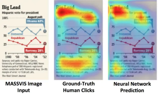
The MASSVIS dataset is rich with manual annotations, eye fixations, memorability scores, and more. In this work, we leverage the data from one of their BubbleView experiments. In this experiment, Mechanical Turk workers are asked to caption a blurred data visualization and can click to deblur regions of interest. The experiment provides us with two valuable pieces of information for each image: click data for visually relevant regions and human captions. We use a Visual Importance Predictor trained on these clicks developed in [7]. The system outputs a heat map the same size as the original image with each pixel value proportional to its predicted importance. An example of a prediction along with it’s ground-truth click importance can be seen in Figure 3-2.
3.2.2
Text extraction
It is tempting to think that because text displayed on a computer is often easy to highlight, copy, and paste, it is easy to extract text from an image, but this intuition is missing a key detail. One must consider that, unlike text-editing software, images store text as an array of pixels, not as ASCII-encoded characters. For example, consider the difference between copying and pasting text from a word document, as opposed to trying to copy and paste text from a photo of a street sign. For our text extraction, we rely almost entirely on the Gupta et al. Oxford Text Spotter, fine-tuned for natural images [10] as seen in Figure 3-3.
Figure 3-2: The input, ground-truth importance, and predicted output importance for an image from the MASSVIS dataset using the Visual Importance Predictor neural network.
Figure 3-3: An example input (left) and extracted text output (right) from the Oxford Text Spotter.
We run the Oxford Text Spotter with highest recall, lowest precision setting (most) so that we can extract the largest number of words possible, even with the additional cost of some false positives. If the extracted text is not a number or numerical quantity (e.g. a percent or dollar amount), we do some basic spell checking using Python’s autocorrect package.
Figure 3-4: Top: Text Spotter at a single scale on an input image with many false posi-tives. Bottom: A result from our improved system which consolidates results from multiple scales, effectively eliminating many false positives.
We made a substantial improvement to the system by reducing the number of false positives. This process involves multi-scale text extraction. We leverage the following observation: false positives are not detected as consistently as true positives when the image is fed into the system at different scales. We feed the input image into the system at the original, 2x, 3x, and 4x scale. We consolidate the results by considering a result the same across scales if any two text boxes’ intersection over union (IOU) is greater than 70%. If a detected text box is consistent across all scales, the result is kept. We also keep results that had less than 0.5 average Levenshtein Distance per letter across scales. The rest were discarded as false positives. A result from our improved system can be seen in Figure 3-4.
3.2.3
Ranking
Once we extract the text, we explore the best ways to assign a relevance scores for keyword identification.
We decide to use the Visual Importance Predictor [7], as this is trained on a metric which highlights what text people look at. As additional baselines, we also consider two saliency metrics, DeepGaze [18] and Judd [15].
After viewing the data visualizations, we suspected that text near the top (e.g. the title) may be good key words. For this reason, we also rank the text by their size and Y-location. Last, we evaluate a random ordering of the words as a shuffled baseline. We report results on 202 test images, each with multiple human captions.
3.3
Results
A schematic of our system can be seen in Figure 1-2. We evaluate our results with the mean Average Precision (AP) metric against words used by at least 7 of the Mechanical Turk captioners. The quantitative evaluation results can be seen in Table 3.1. Note that the Visual Importance Predictor from [7] performs better than most other metrics except for the simple Y-location. DeepGaze produces comparable results while Judd saliency is not much better than a random ranking.
We suspect that Y-location performs so well because of how our evaluation is con-ducted. In particular, as described in Section 3.2.1, participants were asked to provide a short caption of the data visualization, which might bias participants toward reiterating titles located at the top of the image. If, for example, we instead asked participants to pro-vide a list of key words from the visualization, our Predicted Importance ranking may have produced stronger results.
To demonstrate our ranking qualitatively across visualizations and highlight a potential application, we created a simple retrieval demo. In this demo, a user can search visualiza-tions that contain a query word. The results are returned in order of the query’s predicted importance in the visualization. A few results sorted for the search query “Japan" can be seen in Figure 3-5.
Method Mean AP Y-location 0.292 Predicted Importance 0.277 DeepGaze 0.277 Bubble Clicks 0.273 Box Size 0.252 Judd 0.196 Shuffled Baseline 0.183
Table 3.1: The mean AP results for our ranked text extraction method and baselines on words used by a minimum of 7 participants. The methods are sorted in order of importance.
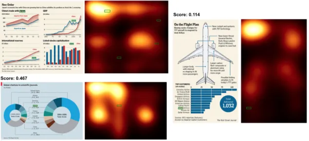
Figure 3-5: Results for querying “Japan" sampled from the top, middle, and bottom of the search results. The retrieved image is shown adjacent to its predicted visual importance. Note that Japan is in a visually important region in the top image, in a moderately important position in the bottom image, and in a subtle location in the right image. The scores are achieved by summing the maximum importance heatmap value contained in the query’s bounding box.
After building such a system that is able to extract and identify the key words in a data visualization, we start to explore other ways to leverage the extracted text. Is it possible to predict the topic of the data visualization from this extracted text, even if the topic word is not used directly? Can we also use visual features to inform our prediction?
Chapter 4
Category and tag prediction
4.1
Problem
After viewing an infographic, a person can assign a topic (category) and a few subtopics (tags) even if those words are not used in the image itself. Inspired by this ability, we focus on predicting categories and tags on the Visually dataset. Given an infographic as input, our goal is to predict one category (of 26) and one or more text tags (of 391). An example of an infographic with its corresponding category and tags is shown in Figure 4-1.
4.2
Approach
Infographics are composed of a mix of textual and visual elements, which combine to generate the message of the infographic. We train both textual and visual models on the category and tag label prediction problems. We use a mean Word2vec representation to transform the extracted words into an input for the text neural network. For visual predic-tion, we use a patch-based multiple instance learning (MIL) framework.
4.2.1
Text to labels
Given an infographic encoded as a bitmap as input, we detected and extracted the text, and then used the text to predict labels for the whole infographic. These labels come in two
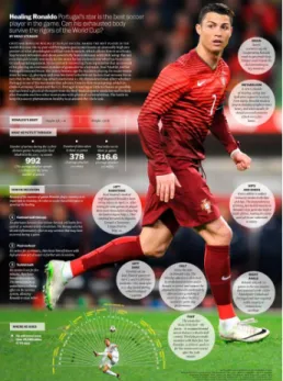
Figure 4-1: An example infographic about the soccer player Ronaldo recovering from an injury to play in the FIFA World Cup. The image’s overall topic or category is “Sports" while its subtopics or tags would be #world cup, #soccer, and #injury. For a full list of the 26 possible categories, refer to the rows of Figure 4-3. For a full list of the 391 tags, refer to the table in Appendix A.
forms: either a single category per infographic (1 of 26), or multiple tags per infographic (out of a possible 391 tags).
Automatic text extraction: We used the previously mentioned Oxford Text Spotter [10] to discover text regions in our infographics. We automatically cleaned the text using spell checking and dictionary constraints in addition to the ones already in [10] to further improve results. We did not apply the multi-scaling presented in Chapter 3 as these images were very large in their original size. On average, we extracted 95 words per infographic (capturing the title, paragraphs, annotations and other text).
Feature learning with text: For each extracted word, we computed a 300-dimensional Word2vec representation [21]. The mean Word2vec of the bag of extracted words was used as the text descriptor for the whole image (the global feature vector of the text). We constructed two simple single-hidden-layer neural networks for predicting the category and tags of each infographic. Category prediction was set up as a multi-class problem, where each infographic belongs to 1 of 26 categories. Tag prediction was set up as a multi-label
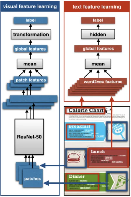
Figure 4-2: Our proposed approach separately samples and processes visual (left/blue) and text regions (right/red) from an infographic to predict labels automatically. Multiple image patches are sampled in a multiple instance learning formulation, and their predictions are averaged to produce the final classification. Text regions are automatically localized, ex-tracted, and converted into Word2vec representations. The average Word2vec representa-tion is then fed into a single hidden layer neural network to produce the final classificarepresenta-tion.
problem with 391 tags, where each infographic could have multiple tags (Table 2.1). The network architecture is the same for both tasks and is depicted in the red box in Figure 4-2, where the label is either a category or multiple tags. We used 26K labeled infographics for training and the rest for testing.
4.2.2
Image patches to labels
Separately from the text, we learned an association between the visual features and category and tag labels.
Working with large images: Since we have categories and tags for all the images in the training data, a first attempt might be to directly learn to predict the category or tag from the whole image. However, the infographics are large images often measuring beyond 1000x1000 pixels. Resizing the images reduces the resolution of visual elements which might not be perceivable at small scales. In particular, relative to the full size of the infographic, many of the pictographs take up very little real-estate but could otherwise contribute to the label prediction. A fully convolutional approach with a batch of such large images was infeasible in terms of memory use. As a result, we sampled the images using both random crops of a fixed size and object proposals from Alexe et al. [1]. We ran the full images resized as a prediction baseline.
Multiple instance learning (MIL) prediction: Given a category or tag label, we ex-pect that specific parts of the infographic may be particularly revealing of that label, even though the whole infographic may contain many diverse visual elements. A multiple in-stance learning (MIL) approach is appropriate in this case. In MIL, the idea is that we may have a bag of samples (in this case patches) to which a label corresponds. The only constraint is that at least one of the samples correspond to the label; the other samples may or may not be relevant.
We used the deep MIL formulation from Wu et al. [30] for learning deep visual repre-sentations. We passed each sampled patch from an infographic through the same convo-lutional neural network architecture, and aggregated the hidden representations to predict a label for the whole bag of patches (depicted in the blue box in Figure 4-2). For
aggre-gating the representations, we tried both element-wise mean and max at the last hidden layer before the softmax transformation, but found mean worked better. As in the text case, we solved either a multi-class category prediction problem, or a multi-label tag prediction problem.
Feature learning with patches: We sampled 5 patches from each infographic and resized each to 224x224 pixels for input into our convolutional neural network. For feature learning, we used ResNet-50 [11], a residual neural network architecture with 50 layers, initialized by pretraining on ImageNet [25]. We retrained all layers of this network on 26K infographics with ground truth labels.
4.2.3
Technical details
Text model: For category prediction, the mean Word2vec feature vector of an infographic was fed through a 300-dimensional fully-connected linear layer, followed by a ReLu, and an output 27-dimensional fully-connected linear layer (including a background class). The feature vectors of all 29K training images fit in memory and could be trained in a single batch, with a softmax cross-entropy loss. For tag prediction, the final fully-connected linear layer was 391-dimensional and was passed through a sigmoid layer. Given the multi-label setting, this network was trained with binary cross-entropy (BCE) loss and one-hot encoded target vectors. Both neural networks were trained for 20K iterations with a learning rate of 1𝑒 − 3.
Visual model: We found that bags of 5 patches in batches of 20 infographics performed best for aggregating visual information from infographics. We also tried bags of 3 patches in batches of 33, patches of 10 in batches of 10. We used a single patch in a batch of 50 infographics as a baseline. As in the text model, we trained category classification with a softmax cross-entropy loss with 27-dimensional target vectors, and tag prediction with a BCE loss applied to 391-dimensional sigmoid outputs. We used a momentum of 0.9 and weight decay of 1𝑒 − 4. Our learning rate was initialized at 1𝑒 − 2 and dropped by a factor of 10 every 10 epochs, for a total of 200 epochs.
4.3
Results
We evaluate the ability of our full system to predict category and tag labels for infographics. Predicting the category label is a high-level prediction task about the overall topic of the infographic. Predicting the multiple tag labels for an infographic is a finer-grained task of discovering sub-topics. We solve both tasks, and present results of our text and visual models.
4.3.1
Category prediction
Quantitative results: For each infographic, we measured the accuracy of predicting the correct ground truth category out of 26, when producing the most confident prediction. Chance level for our distribution of infographics across categories was 15.4%. We achieved 43.2% top-1 accuracy at predicting the category using our text model (Table 4.1). The best performing purely visual system was the MIL framework (as in Figure 4-2) applied to random patches, whose predictions were aggregated using their mean (Vis-rand-mean). We found that mean aggregation outperformed max aggregation for category prediction (Vis-rand-meanbetter than Vis-rand-max). Random crops outperformed object proposals (Vis-rand-meanbetter than Vis-obj-mean), which we hypothesize is the case because they were more consistent, whereas object proposals had diverse aspect ratios and sizes, sometimes too small to capture meaningful visual features. The patch-based predictions were similar to or better than the full visualization resized (Vis-resized). A patch-based approach is naturally better suited for sampling regions for visual tag extraction (Chapter 5). Note that the visual features are not intended to be comparable to the text features, as the text tends to contain a lot more information. We also tried to combine text and visual features directly during training but did not achieve gains in performance above the text model alone, indicating that it is a sufficiently rich source of information in most cases. More baselines are provided in Appendix B.
Automatic text extraction: Given that the automatic text extraction system of [10] was designed for natural images, we benchmarked how well this system performs on in-fographics images. For this purpose we used the 1193 images in the 63K Visually dataset
Model Top-1 Top-3 Top-5 Text-mean 43.2% 69.3% 79.4% Vis-rand-mean 29.4% 51.1% 63.7% Vis-obj-mean 26.1% 48.8% 61.4% Vis-rand-max 26.1% 48.7% 62.3% Vis-resized 23.7% 47.2% 60.0% Vis-obj-max 20.7% 42.6% 57.0% Chance 15.4% 33.6% 47.5%
Table 4.1: Results on category prediction. Models sorted in order of top-1 performance.
that contain full transcripts. For word-level matching, we converted both ground truth tran-scripts and extracted text into bags of words, and found that the extracted text predicts the ground truth text with a precision of 45.7% and recall of 23.9% (5 of the images failed to generate any text).
We also measured category prediction performance if we were able to extract all text accurately and were not limited to the automatically extracted text. Running our text pre-diction model on the Word2vec representation of the transcript words, we obtain a top-1 prediction accuracy of 52.9%, top-3 of 83.2%, and top-5 of 91.0% (training and testing on the reduced set of transcript-containing infographics). Compared to the first row of Ta-ble 4.1, although parsing all the text in an infographic can provide a prediction boost, we note that not all text needs to be perfectly extracted in order to have a good prediction for the topic of an infographic.
Top activations per category: To validate that our visual network trained to predict categories learned meaningful features, we visualize the top 10 patches that received the highest confidence under each category. We provide the patches with the highest confidence under the classifier for each of the 26 categories in Figure 4-3. These patches were obtained by sampling 100 random patches from each image, storing the single patch that maximally activated for each category per image, and outputting the top 10 patches across all images.
4.3.2
Tag prediction
Evaluation: Each infographic in our 29K dataset comes with an average of 1-9 tags. At prediction time, we generate 1, 3, and 5 tags, and measure precision and recall of these
Figure 4-3: The top activating patches per category for all 26 categories from our Visually dataset. We sampled 100 random patches per infographic from all of our test infographics, and picked the patches with highest confidence under our visual network trained to predict category labels. We only picked one patch per infographic to show diversity.
Model Acc. Top-1 Top-3 Top-5 Text-mean-snap prec 45.2% 26.3% 18.9% rec 42.0% 49.0% 53.5% Text-mean prec 27.7% 18.1% 14.0% rec 16.0% 29.5% 37.2% Vis-rand-mean prec 12.2% 8.4% 6.9% rec 6.7% 13.1% 17.8% Vis-rand-max prec 12.2% 8.4% 6.5% rec 6.8% 13.0% 16.8% Vis-resized prec 12.1% 8.2% 6.8% rec 6.5% 13.1% 17.8% Vis-obj-mean prec 11.4% 8.1% 6.6% rec 6.4% 12.6% 17.0% Vis-obj-max prec 11.1% 8.1% 6.4% rec 6.1% 12.5% 16.4% Chance prec 8.7% 6.4% 5.5% rec 5.1% 10.3% 14.3%
Table 4.2: Results on tag prediction. Models sorted in order of top-1 performance.
predicted tags at capturing all ground truth tags for an image, for a variable number of ground truth tags.
Quantitative results: We achieved 45.2% top-1 average precision at predicting at least one of the tags for each of our infographics, since all the infographics in our dataset contain an average of 2 tags (Table 4.2). Since tags are finer-grained than category labels, it is often the case that some word in the infographic itself maps directly to a tag. Using this insight, we add a simple automatic check: if any of the extracted words exactly match any of the 391 tags, we snap the prediction to the matching tags (Text-mean-snap). Without this additional step, predicting top-1 tag achieves an average prediction of 27.7% using text features. We provide the visual model scores for reference, although they are not directly comparable.
Text can disambiguate visual predictions: In some infographics, visual cues for par-ticular tags or topics may be missing (e.g., for abstract concepts), they may be misleading (as visual metaphors), or they may be too numerous (in which case the most representative must be chosen). In these cases, label predictions driven by text are key, as in Figure 4-4, where visual features might seem to indicate that the infographic is about icebergs, ocean, or travel; in this case, however, iceberg is used as a metaphor to discuss microblogging and social media. Our text model is able to pick up on this detail, and direct the visual features
Figure 4-4: Examples of how text and visual features can work together to predict the tags for an image. (a) In “Microblogging iceberg," visual features activate on the water and boats and predict #travel. The text features disambiguate the context, predicting #social media. Conditioned on this predicted tag, the visual features activate on the digital device icons. (b) In this comic about #love and sex, both textual and vision features predict #hu-mor, a correct tag nevertheless. (c) In this infographic about “Dog names," most of the text lists dog names, specialized terms that the text model can not predict the correct tag #animalfrom. The visual features activate on the dog pictographs and make the correct tag prediction.
to activate in the relevant regions.
4.4
User study
4.4.1
Data collection
We designed a user interface to allow participants to both see a visualization all-at-once (resized), and to scroll over to explore any regions in detail using a zoom lens (Figure 4-5). Participants were instructed to provide “5 hashtags describing the image." We collected a total of 3940 tags for the 330 images from 82 Amazon Mechanical Turk workers (an
Figure 4-5: Task used to gather ground-truth human annotations for text tags. Participants could scroll over an image to zoom in and inspect parts of it in order to generate a set of representative tags for the image.
average of 13.3 tags per image, or 2-3 participants/image).
4.4.2
Evaluating the text tags
We compared the collected tags to existing Visually ground truth tags by measuring how many of the ground truth tags were captured by human participants. Aggregating all par-ticipant tags per image (2-3 parpar-ticipants per image), we found an average precision of 37% at reproducing the ground truth tags. After accounting for similar word roots (e.g., #gun matches #handgun), average precision is 51%. This shows that even without a fixed list of tags to choose from (the 391 in our dataset), online participants converge on similar tags as the designer-assigned tags. In other words, the tags in this dataset are reproducible and generalizable, and different people find similar words representative of an infographic.
Furthermore, of all the tags generated by our participants, on average 37% of them are verbatim words from the transcripts of the infographics. This is additional justification for text within infographics being highly predictive of the tags assigned to it.
Knowing that the embedded text performs much better as a predictor of the info-graphic’s category and tags, we next explore whether the embedded text can be used as a supervisory signal for the visual features.
Chapter 5
Visual tag discovery
Text tags as described in Chapter 4 can serve as key words describing this message to facilitate data organization, retrieval from large databases, and sharing on social media. Analogously, we propose an effective visual digest of infographics via visual tags. Visual tags are iconic images that represent key topics of the infographic.
Unlike most natural images, infographics often contain embedded text that provides meaningful context for the visual content. We leverage the text prediction system devel-oped in Chapter 4 to predict text tags. We then use these predictions to constrain and disambiguate the automatically extracted visual features.
This disambiguation is a key step to identifying the most diagnostic regions of an in-fographic. For instance, if the text on an infographic predicts the category “Environment," then the system can condition visual object proposals on the presence of this topic and highlight regions relating to “Environment." In the case of the infographic in Figure 5-1, this disambiguation allows our system to focus on the water droplet and spray bottle, as opposed to the books and light bulb highlighted by “Education."
5.1
Problem
Given an infographic as input, our goal is to identify the input’s visual tags. We evaluate the quality of visual tags by comparing the system’s output to the image regions humans annotate as pertaining to a particular text tag on a given image.
Figure 5-1: Our visual network learns to associate visual elements like pictographs with category labels. We show the activations of our visual network conditioned on different category labels for the same infographic. Allowing the text in an infographic to make the high-level category predictions constrains the visual features to focus on the relevant image regions, in this case “Environment," the correct category for the image. Image source: http://oceanservice.noaa.gov/ocean/earthday-infographic-large.jpg
5.2
Approach
We saw in Chapter 4 that the embedded text in an infographic is often the strongest pre-dictor of the topic matter. Driven by these results, we make label predictions using the text and then constrain the visual network to produce activations for the target label.
At inference time, we sample 3500 random crops per infographic. To generate each crop, we sampled a random coordinate value for the top left corner of the crop, and a side length equal to 10-40% of the minimum image dimension. For each crop, we compute the confidence, under the visual classifier, of the target label. We assign this confidence score to all the pixels within the patch, and aggregate per-pixel scores for the whole infographic. After normalizing these values by the number of sampled patches each pixel occurred in, we obtain a heatmap of activations for the target label. We use this activation map both to visualize the most highly activated regions in an infographic for a given label, and to extract visual tags from these regions.
We first threshold the activation heatmap for each predicted text tag, and identify con-nected components as proposals for regions potentially containing visual tags. These are cropped and passed to the SharpMask segmentation network [23]. This step is important for two reasons: (1) to refine bounding boxes to more tightly capture the contained ob-jects, and (2) to throw out bounding boxes that do not contain an object. During automatic cleaning, we throw out bounding boxes with an area smaller than 5000 pixels, with skewed aspect ratios, or containing more than 35% text (as detected by the pipeline provided by
Figure 5-2: Samples of visual tags extracted for different concepts.
[31]). Furthermore, SharpMask object proposals covering greater than 85% or less than 10% of the bounding box are deemed spurious and thrown out. Finally, visual tags corre-sponding to the predicted text tags for an input infographic are obtained by cropping tight bounding boxes around the remaining proposals (Figure 5-2).
5.3
Results & user study
Results from our visual tagging pipeline can be seen in Figures 5-3 and 5-5. Examples of visual tags discovered across multiple infographics can be seen in Figure 5-2.
The Visually dataset comes with categories and text tags, but not visual tags. Neverthe-less, we wanted to evaluate how well our model learns to localize visual regions relevant to the image-level labels after patch-based MIL training. In order to do this, we crowdsourced object-level annotations on a subset of the test images.
To evaluate our computational model for visual tag extraction, we separately evaluate different steps in the pipeline. First, we evaluate how well our visual model can discover (i.e. activate on) image regions relevant to a text tag. Second, we evaluate the quality of the final visual tags extracted from an image. We compare our visual tag proposals to human bounding box annotations for the same image-tag pairs.
5.3.1
Data collection
We designed an interface in which participants are given an infographic and a target text tag, and are asked to mark bounding boxes around all non text-regions (e.g., pictographs) that contain a depiction of the text tag (Figure 5-4). We used the designer-assigned text tags
(a)
(b)
Figure 5-3: Examples of automatic text and visual tag generation. (a) Text features predict half the ground truth tags correctly, and the visual model discovers associated visual regions in the infographic. Unique visual tags are automatically retrieved for each text tag. (b) Text features predict the ground truth tags correctly, and visual features discover visual tags. In this specific example, there is not a one-to-one mapping between text and visual tags. Similar visual areas are activated for these text tags.
Figure 5-4: Task used to gather ground-truth human annotations for visual tags. Partici-pants annotated visual regions matching text tags.
from the Visually dataset. If an image had multiple text tags, it would be shown multiple times but to different users, with unique image-tag pairings. We collected a total of 3655 bounding boxes for the 330 images from 43 undergraduate students. Each image was seen by an average of 3 participants and we obtained an average of 4 bounding boxes per image. Our visual tagging task required participants to annotate bounding boxes around objects or pictographs in infographics that matched a particular text tag. To ensure the task was well understood and carefully done, we collected the annotations from undergraduate students. Each of our 43 participants annotated an average of 14.7 images and produced an average of 85 bounding boxes (with 15 minutes of effort).
5.3.2
Evaluating the visual model activations
Given an image-tag pairing, participants annotated relevant visual regions. Analogously, given an image-tag pair, we can measure how well our visual model automatically discovers relevant visual regions. We evaluate whether the high-intensity regions in the activation heatmap correspond to the participant-generated annotations. Because each image-tag pair was annotated by 1-3 participants, we report 3 evaluations, measuring how well our model
captures: (A) all the annotations on an image, (B) only annotations on regions made by more than one participant, (C) at least one of the annotations on an image. Note that (A) assumes that the union of all annotations offers a more complete picture; (B) depends on participant consistency and can generate cleaner annotation data; (C) is the most lenient setting where we just care that our model picks a reasonable region of an image. While (A) and (B) can allow us to directly measure the computational limitations of our model, (C) can help us evaluate how well our model would do in practical settings.
For each image-tag pair, we normalize the activation heatmap from our model to be 0 mean, 1 standard deviation. We compute (i) the mean activation value within the annotated regions across all images. A mean activation value above 0 indicates that annotated regions were predicted more relevant than other image regions, on average; (ii) the percent of images for which the mean activation value in annotated regions was above chance (we take chance to be the mean activation value); (iii) the percent of images for which the mean activation value in annotated regions was one standard deviation above the mean. Table 5.1 contains the results.
Evaluation (A) (B) (C) (i) Mean activation value
(across tags)
0.26 0.36 0.86
(ii) Above chance activa-tions (across images)
65% 73% 91%
(iii) Most significant acti-vations (across images)
8% 13% 48%
Table 5.1: Evaluations of how well our model captures: (A) all the relevant visual regions (i.e., all the bounding box annotations on an image), (B) relevant visual regions agreed on by multiple participants, (C) at least one of the relevant regions per image.
5.3.3
Evaluating the extracted visual tags
We collected an average of 4 human-annotated bounding boxes per image-tag pair (for the 330 test infographics). Our automatic pipeline generated an average of 1-2 predicted visual tags per image-tag pair for the same set of infographics, represented as crops from the image.
For each image-tag pair, we measure the intersection-over-union (IOU) of all of our predicted tags to the human annotations. Specifically, for each predicted visual tag, we compute its IOU to the nearest annotated bounding box. We then average the IOU values across all the predicted visual tags for an image-tag pair. The mean IOU over all image-tag pairs is 0.15.
Our pipeline was constructed for high-precision as opposed to high-recall: For a predicted visual tag to be generated, (1) it must have activated our visual model for a given text tag, (2) it must have been fully encapsulated by an image region within the 80th
percentile of the activation map, and (3) it must have been robustly detected by SharpMask as containing an object. As a result, we only produce 1-2 visual tags per image, since our motivation is to produce some diagnostic visual elements to represent the image content rather than extract all visual elements. Figure 5-5 contains some examples. Despite never being trained to explicitly recognize objects in images, our model is able to localize a subset of the human-annotated visual regions.
Figure 5-5: Some sample visual tag extraction results. We show multiple steps of our pipeline: given a text tag, the activation heatmap indicates the image regions that our visual model predicts as most relevant. This heatmap is then passed to our pipeline that extracts visual tags, using objectness and text detection to filter results. The final extracted visual tags are included. We overlay our proposed visual tags (in blue) with human-annotated bounding boxes (in red) of relevant visual regions to the text tag.
Chapter 6
Conclusion
6.1
Contributions and discussion
To this point, the space of complex visual information beyond natural images has received limited attention in computer vision (notable exceptions include: [32] [17]). We present a novel direction to help close this gap. We first explore extracting all words from an image and determining which words are most important to the data visualization. We then leverage these extracted words to predict the topic of the infographic. Finally, we let the text guide our system as its prediction is used to look for corresponding visual cues. In summary, in this research, we
∙ curated a dataset of 29k infographics with 26 categories and 391 tags.
∙ created and evaluated an end-to-end ranked text extraction system for data visualia-tion retrieval.
∙ demonstrated the utility of a patch-based, multiple instance approach for processing large and visually rich images.
∙ created and evaluated an end-to-end category/tag predictor for infographics.
∙ introduced the problem of visual tag discovery: extracting visual regions diagnostic of key topics.
∙ demonstrated the power of extracting text from within an infographic to facilitate visual tag discovery.
∙ created and evaluated an end-to-end visual tag extractor for infographics.
6.2
Looking forward
Although we are pleased with the progress achieved through this research, we have only touched the surface of what we would like to explore in the data visualization understanding domain.
Icon detection: One area of improvement is our localization and extraction of visual tags. Once we identify regions pertaining to a given subtopic, we use an object segmen-tation pipeline tuned for natural images (SharpMask). Also, to train many of our models in the MIL approach, we take crops considered to have high objectness (using models that are also trained on natural images). These models perform poorly on our dataset. Creat-ing an “objectness detector" for infographics, perhaps to be called an “iconness detector," may substantially improve the visual tag extraction pipeline to make it a robust system as opposed to a nice proof-of-concept. This detector might be a sliding window binary-classifier that takes in an image patch and outputs a probability that the input image is a valid icon/object in the infographic.
Dense annotation: Recent research has focused on densely annotating natural images as seen in Figure 6-1a. One can imagine working toward the same goal in data visualiza-tions. So far, our research has focused on a holistic understanding of the data visualization, with visual tag extraction being the preliminary exploration into a finer-grained annotation. A similar system presented in [14] for data visualizations could be a promising research direction.
Data visualization generation: Through this research, we have developed systems that can process a visualization as input and output relevant insights. It might be interesting to consider the flipped task, where we can generate visualizations or visualization elements from the insights we would like to communicate. In natural images, generative adversarial networks (GANS) have shown that we can synthesize realistic looking images from a text
(a) (b)
Figure 6-1: (a) An example of a natural image densely annotated from the pipeline pre-sented in [14]. (b) An image generated from text using the pipeline prepre-sented in [24]. A natural follow-up for purposes of our research domain is: what would it mean to create such systems for data visualizations?
description as seen in Figure 6-1b [24]. What if we could generate new icons to place in visualizations based on the desired object and style? What if we could go even farther and create an entire visualization from a news article?
Data visualizations are specifically designed with a human viewer in mind, character-ized by a high-level message. Beyond simply inferring key words and extracting objects contained within them, a greater understanding of these images would involve a deeper comprehension of the embedded text, the spatial relationship of the elements, the content creator’s intent, and more. We believe this research has taken steps toward this greater understanding, highlighting the potential for computers to work with data visualizations as well as humans and beyond.
Appendix A
Visually dataset
Tag selection: The original tags scraped from the Visually website are free text input by the designer, so many of them are not discriminative, semantically redundant, or have too few instances.
We first manually remove tags considered not sufficiently informative or discriminative (e.g. generic tags like “data_visualization”, “fun_facts” or years like “2015”). The list of manually excluded tags can be seen in Table A.
We merge redundant tags automatically with WordNet and manually. We use Word-Net’s morphological processing module, morphy (e.g. “dog” and “dogs” are both mapped to “dog”). We did additional manual mapping to capture subtle semantic equivalences like “app” and “application.” We also include some mappings to avoid incorrect morphy outputs (like ensuring “hr” maps to “human_resources” instead of “hour”). The manual mappings can be seen in Table A. Finally, as described in the paper, we only keep tags with at least 50 image instances. The trade-off between minimum number of instances and number of remaining images can be seen in Figure A-1. This process results in the final set of 391 tags we use for this dataset (Table A.3).
Image sizes: We constrained the images to be between an aspect ratio of 5:1 or 1:5, inclusive. Of the training images, the widest image is 2840x1000, and the tallest ones (59 such images) are 1000x5000. 4822 are wide images, and 21258 are tall images. 66.5% images have their aspect ratio within 1:3 if it’s a tall image, or 3:1 if it’s a wide image. Moreover, 33.9% images are larger than 1000x1500, and of these 23.4% are larger even
Figure A-1: A graph showing the number of visualizations left and tags included at vari-ous minimum instance thresholds. Each datapoint is labeled with three values: (number of visualizations remaining, number of tags remaining, minimum number of instance guaran-teed per tag). We felt that 50 instances guaranguaran-teed was reasonable (datapoint boxed in red) before further filtering, giving us the final 29k set.
Figure A-2: Histogram of image sizes in the Visually dataset.
analytics data_visualisation data_visualization fun_facts info_graphics infografia infographic infographic_design infographics millennials statistics stats top_10 2000
2008 2009 2010 2011 2012 2013 2015
Table A.1: Manually removed tags.
Word Synonym(s)
application app, apps, mobile_apps, mobile_app baseball mlb
basketball nba
blog wordpress, blogging business small_business car_accident car_accidents
cell_phone android, sms, mobile_phone, iphone, smartphone, smartphones cloud_computing cloud_technology
customer customer_experience, customer_service e-commerce ebay, online_shopping, ecommerce entrepreneur entrepreneurship
finances personal_finance, save_money, saving_money football nfl, super_bowl
health health_benefits home_buying homes_for_sale human_resources hr
injury personal_injury
marketing ppc, social_marketing, inbound_marketing, online_marketing, inter-net_marketing, social_media_marketing, content_marketing
movies star_wars pest pest_control
seo search_engine_optimization
social_media twitter, facebook, google+, linkedin, instagram, pinterest, so-cial_network, social_networking, social_networks, youtube
survey survey_results tablet ipad
technology_company apple, samsung, microsoft television game_of_thrones travel travel_advice united_nations undp web_design website_design
accident accounting addiction advertising africa agriculture airline airport alcohol america american animal application architecture
art asia australia auto automobile automotive b2b b2b_marketing baby banking baseball basketball beauty beer benefit big_data bike black_friday blog book brain
brand branding brazil budget building business california calorie camera canada cancer car car_accident car_insurance
career cat celebrity cell_phone ceo charity chart child china chocolate christmas city cleaning climate_change cloud cloud_computing coffee college color communication community company comparison computer congress construction consumer content
cooking cost country coupon credit credit_card crime culture customer cycling data dating death debt demographic design designer development diabetes diet digital digital_marketing disease divorce diy doctor dog drink
drinking driving drug e-commerce earth earthquake economic economics economy education election electricity email email_marketing
employee employment energy energy_consumption energy_efficiency engagement england entertainment entrepreneur environment europe event evolution exercise export fact family fashion film finance finances fish fitness flight flowchart food football ford foreclosure france fruit fun funding funny future
gadget game gaming gardening gas gdp gender geography germany gift global google government graph
graphic graphic_design green growth guide gun halloween happiness health health_and_safety health_care health_insurance healthcare healthy healthy_eating higher_education hire history hockey holiday home
home_buying home_improvement hospital hotel house housing how_to human_resources humor illustration immigration income india industry inflation information injury innovation insurance interior_design international
internet investing investment io it italy japan job kid kitchen language law lawyer leadership learning life lifestyle loan london love management
map marijuana market market_research marketing marriage medical medicine medium men mental_health military mobile mobile_marketing mobile_phone mom money mortgage move movie music
nasa nature network new_york new_york_city news nutrition obama obesity ocean office oil olympics online parent pest pet phone photography politics pollution population poster poverty power pregnancy president price productivity property psychology real_estate real_estate_agent realtor recipe recruitment recycle recycling relationship religion renewable_energy research
restaurant resume retail retirement revenue roi running russia safety salary sales savings school science search seo search_engine security shopping singapore sleep smoking soccer social social_media software solar solar_energy
space spain spending sport startup strategy stress student style summer supplement survey sustainability tablet
tax teacher tech technology technology_company television thanksgiving time timeline tip tourism trade training transport transportation travel trend turkey tv tweet typography
uk unemployment united_nations united_states university us usa vacation valentine_day vehicle video video_game virus visualization
war waste water weather web web_design web_development website wedding weight_loss wellness wine winter woman
work workout workplace world world_cup zombie
Appendix B
Category and tag prediction
supplemental material
B.1
Additional baselines
Additional results of our experiments are provided in Table B.1, sorted in order of perfor-mance. We found that random patches in bags of 5 patches per image, trained in batches of 20 infographics performed best, which are the results presented in the main thesis. Here we also report our results on training with patches in bags of 8 (Vis-rand-mean-8patch) and 3 (Vis-rand-mean-3patch). Note that random patches generally outperform object propos-als [1] for all batch sizes (i.e. Vis-rand better than Vis-obj). In the case where we sampled object proposal patches, we selected them out of a precomputed 50 patches per image. To explore whether a larger diversity of sampled patches might improve performance, we pre-computed 200 patches per image (Vis-200obj-mean-5patch) but did not see improvements in performance. We tried an additional object proposal framework, DeepMask [22], by tak-ing the minimum area crop around the DeepMask proposals, but performances were even lower (Vis-dmask-mean-5patch). These results point to the fact that our network might be benefiting from larger patches with more context than fitted object patches that have the additional side-effect of coming in different aspect ratios, which get squashed into squares during training. This phenomena might be why random crops produced the best results.
benefits from looking at patches of the image at higher resolution instead of resizing the whole image. On each training run we sampled only 1 patch per infographic (Vis-rand-1patch and Vis-obj-1patch), in batches of 50 infographics. We outperform this baseline when we use 3 or more patches and aggregate them using either mean or max. We found that taking the element-wise mean of the hidden representations of all the patches was more effective than the max, across most settings of our experiment (Vis-rand-mean is generally better than Vis-rand-max and Vis-obj-mean is generally better than Vis-obj-max). We hypothesize that this is because any one pictograph or visual element in an image might not be predictive enough of the category, and additional context is necessary (i.e. taking multiple patches of the image and averaging their representations).
For category prediction evaluation, we use approximately 200 patches and ensemble predictions from sets of 1, 3, 5, or 8 patches1. For tag prediction evaluation, we take the
mean or max over the 200 patches at once instead of ensembling.
Model Top-1 Top-3 Top-5 Vis-text-joined 39.2% 63.5% 74.8% Vis-rand-mean-8patch 29.2% 51.6% 64.2% Vis-rand-mean-3patch 27.6% 50.8% 62.9% Vis-200obj-mean-5patch 26.1% 50.0% 63.3% Vis-rand-max-3patch 24.1% 47.0% 60.4% Vis-rand-1patch 24.0% 46.1% 59.4% Vis-obj-max-3patch 23.8% 44.9% 59.8% Vis-obj-mean-3patch 23.7% 47.4% 59.8% Vis-obj-1patch 19.8% 41.7% 55.8% Vis-dmask-mean-5patch 18.7% 41.0% 54.9%
Table B.1: Results on category prediction. Models sorted in order of top-1 performance.
B.2
Common confusions
Figure B-1 shows the confusions of the text model on category assignment to infographics (choosing the correct out of 26 categories). Categories like “Economy," “Technology" and “Social Media" are often confused with “Business." Also, the model often gets confused 1For Vis-dmask-mean-5patch, we evaluated on images with as few as 5 patches, so we could not evaluate