An automatic annotation system for audio data containing music

(1)

An Automatic Annotation System for Audio Data

Containing Music

by

Janet Marques

Submitted to the Department of Electrical Engineering and Computer Science in Partial Fulfillment of the Requirements for the Degrees of

Bachelor of Science in Electrical Engineering and Computer Science and Master of Engineering in Electrical Engineering and Computer Science

at the Massachusetts Institute of Technology May 1, 1999

distribute publicly paper and electronic copies of this thesis and to grant others the right to do so.

Author_--Department of Electrical Engineering and Computer Science May 1, 1999 Certified by Tomaso A. Poggio Thesis Supervisor Accepted by _____ Arthur C. Smith Chairman, Department Committee on Graduate Theses

(2)

An Automatic Annotation System for Audio Data

Containing Music

by

Janet Marques

Submitted to the

Department of Electrical Engineering and Computer Science May 1, 1999

In Partial Fulfillment of the Requirements for the Degree of Bachelor of Science in Electrical Engineering and Computer Science and Master of Engineering in Electrical Engineering and Computer Science

ABSTRACT

This thesis describes an automatic annotation system for audio files. Given a sound file as input, the application outputs time-aligned text labels that describe the file's audio content. Audio annotation systems such as this one will allow users to more effectively search audio files on the Internet for content. In this annotation system, the labels include

eight musical instrument names and the label 'other'. The musical instruments are

bagpipes, clarinet, flute, harpsichord, organ, piano, trombone, and violin. The annotation tool uses two sound classifiers. These classifiers were built after experimenting with different parameters such as feature type and classification algorithm. The first classifier distinguishes between instrument set and non instrument set sounds. It uses Gaussian Mixture Models and the mel cepstral feature set. The classifier can correctly classify an

audio segment, 0.2 seconds in length, with 75% accuracy. The second classifier

determines which instrument played the sound. It uses Support Vector Machines and also uses the mel cepstral feature set. It can correctly classify an audio segment, 0.2 seconds in length, with 70% accuracy.

Thesis Supervisor: Tomaso A. Poggio Title: Uncas and Helen Whitaker Professor

(3)

Acknowledgements

I would like to thank all of my research advisors: Tomaso Poggio (my MIT thesis

advisor), Brian Eberman, Dave Goddeau, Pedro Moreno, and Jean-Manuel Van Thong (my advisors at Compaq Computer Corporation's Cambridge Research Lab, CRL).

I would also like to thank everyone at CRL for providing me with a challenging and

rewarding environment during the past two years. My thanks also go to CRL for providing the funding for this research. The Gaussian Mixture Model code used in this project was provided by CRL's speech research group, and the Support Vector Machine software was provided to CRL by Edgar Osuna and Tomaso Poggio. I would also like to thank Phillip Clarkson for providing me with his SVM client code.

Many thanks go to Judith Brown, Max Chen, and Keith Martin. Judith provided me with valuable guidance and useful information. Max provided helpful music discussions and contributed many music samples to this research. Keith also contributed music samples, pointed me at important literature, and gave many helpful comments.

I would especially like to thank Brian Zabel. He provided me with a great deal of help

and support and contributed many helpful suggestions to this research. Finally, I would like to thank my family for all of their love and support.

(4)

Chapter 1 Introduction

1.1 Overview

This thesis describes an automatic annotation system for audio files. Given a sound file as input, the annotation system outputs time-aligned labels that describe the file's audio content. The labels consist of eight different musical instrument names and the label

other'.

1.2 Motivation

An important motivation for audio file annotation is multimedia search retrieval. There are approximately thirty million multimedia files on the Internet with no effective method available for searching their audio content (Swa98).

Audio files could be easily searched if every sound file had a corresponding text file that accurately described people's perceptions of the file's audio content. For example, in an audio file containing only speech, the text file could include the speakers' names and the spoken text. In a music file, the annotations could include the names of the musical instruments. These transcriptions could be generated manually; however, it would take a great amount of work and time for humans to label every audio file on the Internet. Automatic annotation tools must be developed.

(7)

This project focuses on labeling audio files containing solo music. Since the Internet does not contain many files with solo music, this type of annotation system is not immediately practical. However, it does show "proof of concept". Using the same techniques, this work can be extended to include other types of sound such as animal

sounds or musical style (jazz, classical, etc.).

A more immediate use for this work is in audio editing applications. Currently, these

applications do not use information such as instrument name for traversing and manipulating audio files. For example, a user must listen to an entire audio file in order to find instances of specific instruments. Audio editing applications would be more effective if annotations were added to the sound files (Wol96).

1.3 Prior Work

There has been a great deal of research concerning the automatic annotation of speech files. However, the automatic annotation of other sound files has received much less attention.

Currently, it is possible to annotate a speech file with spoken text and name of speaker

using speech recognition and speaker identification technology. Researchers have

achieved a word accuracy of 82.6% for "found speech", speech not specifically recorded

for speech recognition (Lig98). In speaker identification, systems can distinguish

between approximately 50 voices with a 96.8% accuracy (Rey95).

The automatic annotation of files containing other sounds has also been researched. One group has successfully built a system that differentiates between the following sound classes: laughter, animals, bells, crowds, synthesizer, and various musical instruments (Wol96). Another group was able to classify sounds as speech or music with 98.6% accuracy (Sch97). Researchers have also built a system that differentiates between classical, jazz, and popular music with 55% accuracy (Han98).

(8)

Most of the work done in music annotation has focused on note identification. In 1977, a group built a system that could produce a score for music containing one or more harmonic instruments. However, the instruments could not be vibrato or glissando, and there were strong restrictions on notes that occurred simultaneously (Moo77). Subsequently, better transcription systems have been developed (Kat89, Kas95, and Mar96).

There have not been many studies done on musical instrument identification. One group built a classifier for four instruments: piano, marimba, guitar, and accordion. It had an impressive 98.1% accuracy rate. However, in their experiments the training and test data were recorded using the same instruments. Also, the training and test data were recorded under similar conditions (Kam95). We believe that the accuracy rate would decrease substantially if the system were tested on music recorded in a different laboratory.

In another study, researchers built a system that could distinguish between two instruments. The sound segments classified were between 1.5 and 10 seconds long. In this case, the test set and training set were recorded using different instruments and under different conditions. The average error rate was a low 5.6% (Bro98). We believe that the error rate would increase if the classifier were extended either through: labeling sound segments less than 0.4 seconds long, or by increasing the number of instruments.

Another research group built a system that could identify 15 musical instruments using isolated tones. The test set and training set were recorded using different instruments and under different conditions. It had a 71.6% accuracy (Mar98). We believe that the error rate would increase if the classifier were not limited to isolated tones.

In our research study, the test set and training set were recorded using different instruments and under different conditions. Also, the sound segments were less than 0.4 seconds long and were not restricted to isolated tones. This allowed us to build a system that could generate accurate labels for audio files not specifically recorded for recognition.

(9)

1.4 Document Outline

The first chapter introduces the thesis project. The next chapter describes the relevant background information. In the third chapter, the research experiments are described. The fourth chapter is devoted to the presentation and analysis of the experiment results. The last part of the thesis includes directions for future work and references.

(10)

Chapter 2 Background Information

2.1 Introduction

This chapter discusses background information relevant to the automatic annotation system. The system is made up of two sound classifiers. The first classifier distinguishes between instrument set and non instrument set sounds. If the sound is deemed to be made by an instrument, the second classifier determines which instrument played the

sound. For both classifiers, we needed to choose an appropriate feature set and

classification algorithm.

2.2 Feature Set

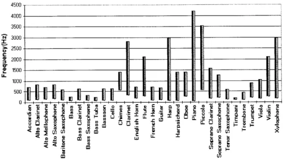
The first step in any classification problem is to select an appropriate feature set. A feature set is a group of properties exhibited by the data being classified. An effective feature set should contain enough information about the data to enable classification, but also contain as few elements as possible. This makes modeling more efficient (Dud73). Finding a feature set is usually problem dependent. In this project, we needed to find features that accurately distinguish harmonic musical instruments. One feature that

partially distinguishes instruments is frequency range. Figure 2.1 illustrates the

(11)

frequency ranges overlap, we can say that harmonic instruments are not uniquely specified by frequency range alone.

4500 -4000 3500- 3000-M 2500 -C 02000. S1500. 1000. C0 C 1 1 0 E 0 0 Cw ₁ _x C C EoU E 0 OW gCC X 6

Figure 2.1 Frequency range of various musical instruments.

Another possible feature set is harmonic number amplitude. Harmonics are the

sinusoidal frequency components of a periodic sound. Musical instruments tend to sound differently because of differences in their harmonics. For example, a sound with intense energy in higher frequency harmonics tends to sound bright like a piccolo, while a sound with high energy in lower frequency harmonics tends to sound rather dull like a tuba (Pie83).

The harmonic amplitude feature set has been successful in some classification problems. In one study, the mean amplitudes of the first 11 harmonics were used as a feature set for the classification of diesel engines and rotary wing aircraft. An error rate of 0.84% was achieved (Mos96). However, we believed that this feature set might not be successful for an instrument classifier. For instance, the feature set is well defined for instruments that can only play one note at a time, such as clarinet, flute, trombone, and violin. However, it was not straightforward how we would derive such a feature set for instruments like

-- - - - - - --- ---- -- -- --- -

(12)

in---piano, harpsichord, and organ. Also, we believed that the harmonic feature set might not contain enough information to uniquely distinguish the instruments. Therefore, we hypothesized that a harmonic amplitude feature set may not be the best feature set for musical instrument classification.

Two feature sets that are successful in speech recognition are linear prediction coefficients and cepstral coefficients. Both feature sets assume the speech production model shown in Figure 2.2. The source u(n) is a series of periodic pulses produced by air forced through the vocal chords, the filter H(z) represents the vocal tract, and the output o(n) is the speech signal (Rab93). Both feature sets attempt to approximate the vocal tract system.

u(n) H(z)n)

Figure 2.2 Linear prediction and cepstrum model of speech production and musical instrument sound production.

The model shown in Figure 2.2 is also suitable for musical instrument sound production. The source u(n) is a series of periodic pulses produced by air forced though the instrument or by resonating strings, the filter H(z) represents the musical instrument, and

the output o(n) represents the music. In this case, both feature sets attempt to

approximate the musical instrument system.

When deriving the LPC feature set, the musical instrument system is approximated using an all-pole model,

G

H

(z)=

,

1-±a

iz-i=1

where G is the model's gain, p is the order of the LPC model, and {ai ... ap} are the model coefficients. The linear prediction feature set is {a, ... ap} (Rab93).

(13)

One problem with the LPC set is that it approximates the musical instrument system using an all-pole model. This assumption is not made when deriving the cepstral feature set. The cepstral feature set is derived using the cepstrum transform:

cepstrum(x) = FFT-1(In

I

FFT(x)|).

If x is the output of the system described in Figure 2.2, then

cepstrum(x)= FFT-'( In IFFT(u(n))

I

)+ FFT-'(ln IH(z)|).

FFT-'( In

IFFT(u(n)) I)

is a transformation of the input into the musical instrument

system. It is approximately a series of periodic pulses with some period No.

FFT-'(ln H(z) |) is a transformation of the musical instrument system.

Since FFT-1(In

IH(z)

|) contributes minimally to the first No -1 samples

of cepstrum(x) , the first No - 1 samples should contain a good representation of the

musical instrument system. These samples are the cepstral feature set (Gis94).

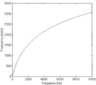
A variation of the cepstral feature set is the mel cepstral set. This feature set is identical

to the cepstral except that the signal's frequency content undergoes a mel transformation before the cepstral transform is calculated. Figure 2.3 shows the relationship between Hertz and mel frequency. This transformation modifies the signal so that its frequency content is more closely related to a human's perception of frequency content. The relationship is linear for lower frequencies and logarithmic at higher frequencies (Rab93). The mel transformation has improved speech recognition results because speech phonemes appear more different on a mel frequency scale than on a linear Hertz scale. Similarly to the distinctness of human phonemes, the musical instruments in this study produce different sounds according to the human ear. Therefore, it was our prediction that the mel transformation would improve instrument classification results.

A feature set type that has not been discussed is temporal features. Temporal features are

most effective for sound signals that have important time-varying characteristics. Examples of such feature sets include wavelet packet coefficients, autocorrelation

(14)

coefficients, and correlogram coefficients. The wavelet feature set has been used in respiratory sound classification and marine mammal sound classification (Lea93). The autocorrelation and correlogram feature sets have been used in instrument classification (Bro98, Mar98). 3500 3000 2500 2000 1500 -1000 500 -0 0 2000 4000 6000 8000 10000 Frequency (Hz)

Figure 2.3 Relationship between Hertz and mels.

A large amount of psychophysical data has shown that musical instruments have

important time-varying characteristics. For example, humans often identify instruments

using attack and decay times (Mca93). Feature sets that exploit time-varying

characteristics are most likely more effective than feature sets that do not use temporal

cues. In one study, a fifteen-instrument identification system using correlogram

coefficients achieved a 70% accuracy rate. The system was trained and tested using individual tones.

In this study, continuous music as opposed to individual tones was examined. Since it is difficult to accurately extract individual tones from continuous music, temporal feature sets were not examined in this research.

One other common feature extraction method is to use a variety of acoustic characteristics, such as loudness, pitch, spectral mean, bandwidth, harmonicity, and

(15)

spectral flux. This method has been successful in many classification tasks (Sch97, Wol96). However, it is difficult to determine which acoustic characteristics are most appropriate for a given classification problem. This type of feature set was not explored in this research.

In this thesis, we examined the following feature sets: harmonic amplitude, linear prediction, cepstral, and mel cepstral.

2.3 Classification Algorithm

After an adequate feature set has been selected, the classification algorithm must be chosen. The Gaussian mixture model (GMM) and Support Vector Machine (SVM) algorithms are discussed below.

2.3.1 Gaussian Mixture Models

Gaussian Mixture Models have been successful in speaker identification and speech recognition. In this algorithm, the training feature vectors for the instrument classifier are used to model each instrument as a probability distribution. A test vector I is classified as the instrument with the highest probability for that feature vector.

Each instrument's probability distribution is represented as a sum of Gaussian densities:

K

p(z|ICi)= P(gi |Ci) p(z Iwi, Cj),

where p(-Iwi,C₁)= (z.)1j

X represents a feature vector, gi represents Gaussian i, C1 represents class

j,

K is the

number of Gaussian densities for each class, P(g,

I

C1) is the probability of Gaussian I

(16)

d-component mean vector for Gaussian i in class

j,

Z. is a d x d covariance matrix for

Gaussian i in class j, (X - U),)'is the transpose of ii - Aj, 1-1 is the inverse of Z,, and

is the determinant of Iii.

The Gaussian mixture used to represent each class is found using the Expectation-Maximization (EM) algorithm. EM is an iterative algorithm that computes maximum likelihood estimates. Many variations of this algorithm exist, but they were not explored in this project (Dem77). The initial Gaussian parameters (means, covariances, and prior probabilities) used by EM were generated via the k-means method (Dud73). Other initialization methods include the binary tree and linear tree algorithms, but they were not explored in this project.

Once a Gaussian mixture has been found for each class, determining a test vector's class is straightforward. A test vectori- is labeled as the class that maximizes p(C I i) which

is equivalent to maximizing p(

I

C )p(Cj) using Bayes rule. When each class has

equal a priori probability, then the probability measure is simply p(Y

I

C₁). Therefore,

the test vector Y is classified into the instrument class C1 that maximizes p(I| C1).

2.3.2 Support Vector Machines

Support Vector Machines have been used in a variety of classification tasks, such as isolated handwritten digit recognition, speaker identification, object recognition, face detection, and vowel classification. When compared with other algorithms, they show

improved performance. This section provides a brief summary of SVMs; a more

thorough review can be found in (Bur98).

Support Vector Machines are used for finding the optimal boundary that separates two classes. We begin with a training vector set,

{,

...

,

Y

}

where -i e R'. Each training

(17)

vector i, belongs to the class y, where y, E {-1, 1}. The following hyperplane separates the training vectors into the two classes:

(W -.)+ b where WE R" , bE R, and yi((WV.-2)+b) >1 V i.

However, this hyperplane is not optimal. An optimal hyperplane would maximize the distance between the hyperplane and the closest samples, iY and X-₂.

2/1W1 which is illustrated in Figure 2.4.

This distance is

Therefore, the optimal hyperplane, (W. -) + b, is found by minimizing W

maintaining y,((W-.)+b)>1 Vi. This problem can be solved with quadratic

programming, and results in W = v . The i are a subset of the training samples that

lie on the margin. (Sch98).

They are called support vectors. The vi are the multiplying factors

*X (-) -b X) =+1 * N~h~: (W X1 b= i1 SyU~%V (w X1 + b=-0 _*,, _=: _{X X =} Y= ..... 0 ....

Figure 2.4 The optimal hyperplane maximizes the distance between the hyperplane and the closest samples, Y, and Y2. This distance is

2/1WI (reproduced from Sch98).

In the previous case, a linear separating hyperplane was used to separate the classes. Often a non-linear hyperplane is necessary. First, the training vectors are mapped into a while

(18)

higher dimensional space, (D(2i.) where D : R" [-- H. Then, a linear hyperplane is found in the higher dimensional space. This translates to a non-linear hyperplane in the original input space (Bur98, Sch98).

Since it is computationally expensive to map the training vectors into a high dimensional space, a kernel function is used to avoid the computational burden. The kernel function

is used instead of computing 'I(1i) - (i7). Two commonly used kernels are the

polynomial kernel, K(Xi, - )= (Y, -Y, +1)' and the Gaussian radial basis function (RBF)

kernel, K(i, 1) = exp( i 1 2) (Bur98). The kernel function used in this

research was K(zi,-) = ( - - +1)'. We chose a polynomial of order 3 because it has+I

worked well in a variety of classification experiments.

We have discussed SVMs in terms of two-class problems, however, SVMs are often used in multi-class problems. There are two popular multi-class classification algorithms, one-versus-all and one-versus-one.

In the one versus one method, a boundary is found for every pair of classes. Then, votes are tallied for each category by testing the vector on each two-class classifier. The vector is labeled as the class with the most votes.

In the one versus all method, we find a boundary for each class that separates the class from the remaining categories. Then, a test vector Y is labeled as the class whose boundary maximizes

|(W-

- -)+ b 1.

(19)

Chapter 3 Classifier Experiments

3.1 Introduction

This chapter outlines the automatic annotation system. It then describes the experiments involved in developing the system.

3.2 Automatic Annotation System

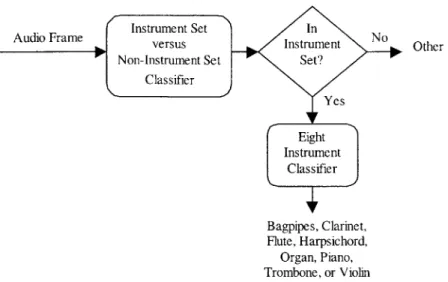
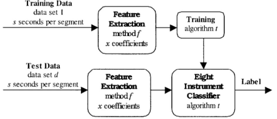
Given a sound file as input, the annotation system outputs time-aligned labels that describe the file's audio content. The labels consist of eight different musical instrument names and the label 'other'. First, the sound file is divided into overlapping segments. Then, each segment is processed using the algorithm shown in Figure 3.1.

The algorithm first determines if the segment is a member of the instrument set. If it is not, then it is classified as 'other'. Otherwise, the segment is classified as one of the eight instruments using the eight-instrument classifier.

After each overlapping segment is classified, the system marks each time sample with the class that received the most votes from all of the overlapping segments. Lastly, the annotation system filters the results and then generates the appropriate labels.

(20)

Audio Frame No b Other Bagpipes, Clarinet, Flute, Harpsichord, Organ, Piano, Trombone, or Violin

Figure 3.1 Algorithm used on each audio segment in the automatic annotation system.

The filter first divides the audio file into overlapping windows s seconds long. Then, it determines which class dominates each window. Each time sample is then labeled as the class with the most votes.

In order for the filter to work correctly, each label in the audio file must have a duration longer than s seconds. If s is too long, then the shorter sections will not be labeled correctly. We believed that the accuracy of the annotation system would be positively correlated with the value of s as long as s was less than the duration of the shortest label.

3.3 Eight Instrument Classifier

The first step in building the eight-instrument classifier was to collect training and testing data. To find the best parameters for the identification system, numerous experiments were conducted.

3.3.1 Data Collection

This part of the project used music retrieved from multiple audio compact disks (CD). The audio was sampled at 16 kHz using 16 bits per sample and was stored in AU file

(21)

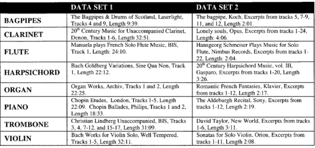
format. This format compressed the 16-bit data into 8-bit mu-law data. The data was retrieved from two separate groups of CDs. Table 3.1 lists the contents of the two data sets.

BAGPIPES The Bagpipes & Drums of Scotland, Laserlight, The bagpipe, Koch, Excerpts from tracks 5, 7-9, Tracks 4 and 9, Length 9:39. 11, and 12, Length 2:01.

CLARINET 2 0_{Denon, Tracks 1-6, Length 32:51.}h Century Music for Unaccompanied Clarinet, Lonely souls, Opus, Excerpts from tracks 1-24,_{Length: 4:06.}

Manuela plays French Solo Flute Music, BIS, Hansgeorg Schmeiser Plays Music for Solo FLUTE Track 1, Length: 24:10. Flute, Nimbus Records, Excerpts from tracks

I-22, Length: 2:04.

Bach Goldberg Variations, Sine Qua Non, Track 2 01h Century Harpsichord Music, vol. III,

HARPSICHORD 1, Length 22:12. Gasparo, Excerpts from tracks 1-20, Length

3:26.

ORGAN Organ Works, Archiv, Tracks 1 and 2, Length Romantic French Fantasies, Klavier, Excerpts

22:25. from tracks 1-12, Length 2:17.

Chopin Etudes, London, Tracks 1-5, Length The Aldeburgh Recital, Sony, Excerpts from PIANO 22:09. Chopin Ballades, Philips, Tracks 1 and 2, tracks 1-12, Length 2:19.

Length 18:33.

TROMBONE Christian Lindberg Unaccompanied, BIS, Tracks David Taylor, New World, Excerpts from tracks

3, 4, 7-12, and 15-17, Length 31:09. 1-6, Length 3:11.

VIOLIN Bach Works for Violin Solo, Well Tempered, Sonatas for Solo Violin, Orion, Excerpts from Tracks 1-5, Length 32:11. tracks 1-11, Length 2:08.

Table 3.1 Data for instrument classification experiments.

After the audio was extracted from each CD, several training and testing sets were formed. The segments were randomly chosen from the data set, and the corresponding training and test sets did not contain any of the same segments. In addition, segments with an average amplitude below 0.01 were not used. This automatically removed any silence from the training and testing sets. This threshold value was determined by listening to a small portion of the data.

Lastly, each segment's average loudness was normalized to 0.15. We normalized the segments in order to remove any loudness differences that may exist between the CD recordings. This was done so that the classifier would not use differences between the CDs to distinguish between the instruments. We later found that the CDs had additional recording differences.

(22)

3.3.2 Experiments

A variety of experiments were performed in order to identify the best parameters for the

identification system. The system is outlined in Figure 3.2. The parameters of concern were test data set, segment length, feature set type, number of coefficients, and classification algorithm.

Training Data

data set Feature ₁

s seconds per segment

arat

t x rain ing

for tet rsodf for t x coefficients

Test Data

data set d _Featur

Eigt Lae

s seconds per segment Ex in Instutnt

01 methodf Classifier P

x coefficiers algorithm t

Figure 3.2 Eight instrument classification system.

Test Data Set refers to the source of the test data. Data sets 1 and 2 were extracted from two separate groups of CDs. It was important to run experiments using different data sets for training and testing. If the same data set were used for training and testing, then we would not know whether our system could classify sound that was recorded under different conditions. In a preliminary experiment, our classifier obtained 97% accuracy when trained and tested using identical recording conditions with the same instruments. This accuracy dropped to 71.6% for music professionally recorded in a different studio, and it dropped to 44.6% accuracy for non-professionally recorded music. The last two experiments used different instruments for training and testing as well.

The drop in accuracy could also be attributed to differences in the actual instruments used and not just the recording differences. If this is true, then it should have been possible for our classifier to distinguish between two instances of one instrument type, such as two violins. In a preliminary experiment, we successfully built a classifier that could

(23)

distinguish between two violin segments recorded in identical conditions with a 79.5% accuracy. The segments were 0.1 seconds long.

Segment Length is the length of each audio segment in seconds. This parameter took one of the following values: 0.05 sec, 0.1 sec, 0.2 sec, or 0.4 sec. For each experiment, we kept the total amount of training data fixed at 1638.8 seconds. We did not expect

segment length to substantially affect performance. A segment longer than 2/27.5

seconds (0.073 seconds) contains enough information to enable classification because

27.5 Hertz is the lowest frequency that can be exhibited by any of our instruments.

Therefore, 0.1 seconds should have been an adequate segment length. We expected some performance loss when using 0.05 second segments.

Feature Set Type is the type of feature set used. Possible feature types include harmonic amplitudes, linear prediction, cepstral, and mel cepstral coefficients.

The harmonic amplitude feature set contains the amplitudes of the segment's first x harmonics. The harmonic amplitudes were extracted using the following algorithm:

1. Find the segment's fundamental frequency using the auto-correlation method.

2. Compute the magnitude of the segment's frequency distribution using the Fast Fourier Transform (FFT).

3. Find the harmonics using the derivative of the segment's frequency distribution.

Each harmonic appears as a zero crossing in the derivative. The amplitude of each harmonic is a local maximum in the frequency distribution, and the harmonics are located at frequencies that are approximately multiples of the fundamental frequency.

An application of this algorithm is demonstrated in Figure 3.3. The frequency

distribution from 0.1 seconds of solo clarinet music is shown in the first graph, and the set of eight harmonic amplitudes is illustrated in the second graph.

The next feature set used was the linear prediction feature set. It was computed using the Matlab function lpc, which uses the autocorrelation method of autoregressive modeling

(24)

(Mat96). The computation of the cepstral and mel cepstral feature sets was discussed in Section 2.2.

Frequency Distribution of 0 1 sec of Solo Clarinet Music 200 150 -100 -50~ 0- -0 1000 2000 3000 4000 5000 Frequency (Hz)

Harmonic Amplitude Feature Set for 0.1 sec of Solo Clarinet Music

150

-o100

-

50-0 1000 2000 3000 4000 5000

Frequency (Hz)

Figure 3.3 Frequency distribution of 0.1 seconds of clarinet music with corresponding harmonic amplitude feature set.

Number of Coefficients is the number of features used to represent each audio segment. This parameter took one of the following values: 4, 8, 16, 32, or 64. If there were an infinite amount of training data, then performance should improve as the feature set size is increased. More features imply that there is more information available about each class. However, increasing the number of features in a classification problem usually requires that the amount of training data be increased exponentially. This phenomenon is known as the "curse of dimensionality" (Dud73).

Classification Algorithm We experimented with two algorithms: Gaussian Mixture Models and Support Vector Machines. SVMs have outperformed GMMs in a variety of classification tasks, so we predicted that they would show improved performance in this classification task as well.

Within each classification algorithm, we experimented with important parameters. In the GMM algorithm, we examined the effect of the number of Gaussians. For the SVM

(25)

algorithm, we examined different multi-class classification algorithms; the popular algorithms being one-versus-all and one-versus-one.

Using various combinations of the parameters described above, we built many classifiers. Each classifier was tested using 800 segments of audio (100 segments per instrument). For each experiment, we examined a confusion matrix. From this matrix, we computed the overall error rate and the instruments' error rates. In the confusion matrix,

r r 2 ... r r21 r22 r2 8

r8 1 r82 '' r88 _

there is one row and one column for each musical instrument. An element ri; corresponds

to the number of times the system classified a segment as instrument

j

when the correct answer was instrument i. The overall error rate was computed as,

8

1 ii

1- 8 8

11r j=1 i=1

and the error rate for an instrument x was computed as,

1 r _

8 8

rX +

x-i=1 j=1

Since each instrument's error rate includes the number of times another instrument was misclassified as the instrument in question, the overall error rate was usually lower than the individual error rates.

(26)

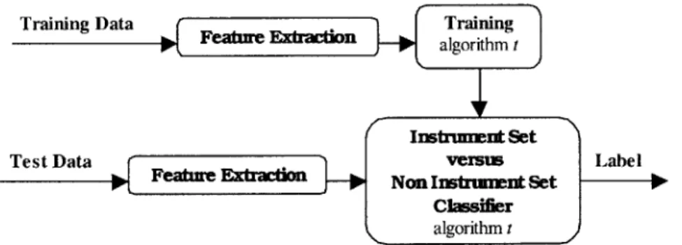
3.4 Instrument Set versus Non Instrument Set Classifier

The first step in building the instrument set versus non instrument set classifier was to collect training and testing data. After this was completed, we performed numerous experiments to determine the best parameters for the classifier.

3.4.1 Data Collection

This part of the project required a wide variety of training data to model the two classes. We used sound from many sources: the Internet, multiple CDs, and non-professional recordings. The audio was sampled at 16 kHz used 16 bits per sample and was stored in

AU file format. This format compressed the 16-bit data into 8-bit mu-law data.

The instrument set class was trained with sound from each of the eight musical instruments. The data for this class is described in Table A.1 in the Appendix. There were 1874.6 seconds of training data and 171 seconds of test data for this class. The data was evenly split between the eight instrument classes. In addition, the training and test data was acquired from two different CD sets, so we were able to test that the classifier was not specific to one set of recording conditions or to one set of instruments.

The non instrument set class was trained with sound from a variety of sources. The data for this class is described in Tables A.2 and A.3 in the Appendix. There were 1107.4 seconds of training data and 360 seconds of test data. It included the following sound types: animal sounds, human sounds, computer sound effects, non-computer sound effects, speech, solo singing, the eight solo instruments with background music, other

solo instruments, and various styles of non-solo music with and without vocals.

There are a number of reasons we chose this training and test data for the non instrument set:

" We used a variety of sounds so that the non instrument model would be general. " The eight instrument sounds with background music were included in the non

(27)

decided that the instrument set class should only include solo music, as our eight-instrument classifier had been trained only with solo eight-instruments. If our classifier worked correctly with non-solo music, then it would have been more appropriate to include sound with background music in our instrument set class.

" The test data included some sounds not represented in the training set, such as the owl

sound. This was done in order to test that the class model was sufficiently general.

e The training and test data were composed of sounds recorded under many different

conditions. Therefore, we were able to test that the classifier was not specific to one set of recording conditions.

3.4.2 Experiments

We performed a variety of experiments in order to identify the best classification algorithm for the identification system. The system is outlined in Figure 3.4. In each experiment, we used a segment length of 0.2 seconds, the mel cepstral feature set, and 16 feature coefficients.

Traiing ata Feature Extrctin a g rinin

Instrnment Set

Test Data jjLFahneK _ versus Label

Featre &Non Instrnmnt Set ---classifier

k, algorithm t

Figure 3.4 Instrument set versus non instrument set classification system.

Support Vector Machines

We used a two-category SVM classifier. The two categories were instrument set versus non instrument set. Researchers have achieved good results with SVMs in similar problems, such as face detection. In one study, using the classes: face and non-face, the detection rate was 74.2% (Osu98).

(28)

Gaussian Mixture Models

We built two types of GMM classifiers, two-category and nine category. For each classifier, each category was modeled using a Gaussian mixture model. Based on the numerous studies demonstrating that SVMs yield better results than GMMs, we predicted similar results in our system.

Two Class

The two classes were instrument set and non instrument set. Given a test sound, the class with the highest probability was chosen. A test vector was then labeled as the class with the largest probability.

Nine Class

The nine classes were non instrument set, bagpipes, clarinet, flute, harpsichord, organ, piano, trombone, and violin. A test vector was labeled as 'other' if the non instrument class had the largest probability. Otherwise, it was labeled as an instrument set member. We thought that the two-class method would work better because it provided a more general instrument model. The two-class model is more general because it used one GMM model to represent all of the instruments, while the nine class method used a

separate GMM model for each instrument. A more general instrument model is

beneficial because the test set used in these experiments was quite different from the training set; it used different instances of the musical instruments and different recording conditions.

Probability threshold

The probability threshold classifier worked in the following manner: given a test vector

x, we calculated p(C I-) for each of the eight instrument classes. If

max(p(C

I

T)) < Te, then the test sound was labeled as 'other'. Otherwise, it was labeled

C

as an instrument set sound. For example, if a test vector Y is most likely a clarinet, and

(29)

'other'. If p( clarinet

I

X-) was greater then the clarinet threshold, then the vector was

labeled as an instrument set sound.

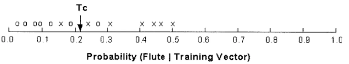
The probability threshold for an instrument C was calculated as follows:

1. The training data was separated into two groups. The first group contained the

training data that belonged in class C, and the second group contained the training data that did not belong in class C. For example, if class C was flute, then the non-flute group would include all of the non instrument set data plus bagpipes, clarinet, harpsichord, organ, piano, trombone, and violin data.

2. For every vector Y in either training set, we calculated the probability that it is a member of class C, p(C

I

X), using the Gaussian mixture model for class C. For

example, the non-flute vectors would have lower probabilities than the flute vectors.

3. The threshold Tc was the number that most optimally separated the two training data

groups. An example is shown in Figure 3.5. In this example, Tc separates the flute probabilities from the non-flute probabilities. The x symbols represent the flute probabilities and the o symbols represent the non-flute probabilities.

Tc

0 000 0 X 0 0, OX X XX X

I14 I I I I I I I I

0.0 0.1 0.2 0.3 0.4 0.5 0.6 0.7 0.8 0.9 1.0

Probability (Flute I Training Vector)

Figure 3.5 The threshold Tc optimally separates the flute probabilities (x) from the non-flute probabilities (o).

In each experiment, we used 2214 seconds of training data. The test data contained 179 seconds of instrument set samples and 361 seconds of non instrument set samples. For each experiment, we examined a 2x2 confusion matrix,

(30)

e rI : the number of times the system classified an instrument set segment correctly.

* r12 : the number of times the system classified a non instrument set segment as an

instrument set segment.

* r21 : the number of times the system classified an instrument set segment as a non

instrument segment.

* r12: the number of times the system classified a non instrument set segment correctly.

The overall error rate was computed as,

1- r22

(31)

Chapter 4 Results and Dis cussion

4.1 Introduction

After performing experiments to determine the most effective classifiers, we built the automatic annotation system. This chapter first presents results for the entire system, and then discusses the results for each classifier in detail.

4.2 Automatic Annotation System

The automatic annotation system was tested using a 9.24 second sound file sampled at 16 KHz. The audio file contained sound from each of the eight instruments. It also contained sound from a whistle. Table 4.1 shows the contents of the audio file. The units

are in samples.

The annotation system first divided the audio file into overlapping segments. The

segments were 0.2 seconds long and the overlap was 0.19 seconds. Then each segment was classified using the two classifiers. Afterwards, each time sample was marked with the class that received the most votes. Lastly, the annotation system filtered the results

and then generated the appropriate labels.

The filter first divided the audio file into overlapping windows 0.9 seconds long. We chose 0.9 seconds because all of the sound sections in the audio file were longer than 0.9

(32)

seconds. Then, the filter determined which class dominated each window. Each time sample was then labeled with the class with the most votes.

Bagpipes 17475 Violin 17476 33552 Clarinet 33553 49862 Trombone 49863 66871 Other 66872 82482 Piano 82483 98326 Flute 98327 115568 Organ 115569 131645 Harpsichord 131646 147803

Table 4.1 Contents of the audio file used for the final test. The units are in samples.

The results are shown in Figure 4.1. The figure contains the audio file waveform, the correct annotations, and the automatic annotations. The error rate for the audio file was 22.4%. We also tested the system without the filter. In that experiment, the error rate was 37.2%.

correct labels: bag vio cia tro oth pia flu org har

auto labels: bag vio cla oth pia flu org har

cla pia

Figure 4.1 Final test results.

The annotation system performed poorly in the trombone section. This was likely because section was generated with a bass trombone, and the system was trained with a tenor trombone.

I

(33)

The filter used in the annotation system decreased the error rate substantially. However, in order for the filter to work optimally, each label in the audio file must have had a duration larger than the window length.

The results for the two sound classifiers are discussed in detail in Sections 4.3 and 4.4. The classifiers used in the final annotation system are described below:

e The eight instrument classifier used the SVM (one versus all) algorithm and the

following parameter settings: 1638 seconds of training data, the mel cepstral feature set, a 0.2 second segment length, and 16 feature coefficients per segment. The error rate for this classifier was 30%. The instrument error rates were approximately equal, except for the trombone and harpsichord error rates. The trombone error rate was 85.7% and the harpsichord error rate was 76.5%. The trombone error rate was high because the classifier was trained with a tenor trombone, and tested with a bass trombone. We believe that the harpsichord accuracy was low for similar reasons.

e The instrument set versus non instrument set classifier used the GMM (two class)

algorithm and the following parameter settings: 2214 seconds of training data, the mel cepstral feature set, a 0.2 second segment length, and 16 feature coefficients per segment. The error rate for this classifier was 24.4%. The test set contained some sound types that were not in the training set. The system classified the new types of sounds with approximately the same accuracy as the old types of sounds.

4.3 Eight-Instrument Classifier

In order to find the most accurate eight-instrument classifier, many experiments were performed. We explored the feature set space (harmonic amplitudes, LPC, cepstral, and mel cepstral), the classifier space (SVM and GMM), and various parameters for each classifier.

(34)

4.3.1 Gaussian Mixture Model Experiments

We first explored GMM classifiers. In addition to feature set type, the following

parameters were examined: number of Gaussians, number of feature coefficients, segment length, and test data set.

Feature Set Type

First, we performed an experiment to find the best feature set. We examined harmonic amplitudes, linear prediction coefficients, cepstral coefficients, and mel cepstral coefficients. The other parameter values for this experiment are listed in Table 4.2.

Data Set for Training CD Set I Classification Algorithm GMM

Data Set for Testing CD Set 1 Number of Gaussians 8

# Training Segments 4096 Feature Set Type

---Training Segment Length 0.1 sec # Feature Coefficients 16 Table 4.2 Parameters for feature set experiment (GMM).

The mel cepstral feature set gave the best results, overall error rate of 7.9% classifying

0.1 sec of sound. Figure 4.2 shows the results. The error rates were low because the

training and test data were recorded under the same conditions. This is explained in more detail in the results section of the test data set experiment.

Overall Error Rate Instrument Error Rates

0 .36 - -

-harrmnics lpc ceps tral rnel ceps tral Features Figure 4.2 Results 0.8 0.7 a0.6 0.5 S0.4 2h 0. 3 LU 0.2 0.1 0

harrmnics [Pc ceps tral

Features -- bagpipes -- clarinet flute harps ichord -- I-- organ -0- piano rnel -+- trorrbone ceps tral - iolin

for feature set experiment (GMM).

The harmonic feature set probably had the worst performance because the feature set was not appropriate for piano, harpsichord, and organ. These instruments are capable of

0 LU 0.45 0.4 0.35 0.3 0.25 02 0.15 0.1 0.05 0

(35)

playing more than one note at a time, so it is unclear which note's harmonics are appropriate to use.

The cepstral set probably performed better than the linear prediction features because musical instruments are not well represented with the linear prediction all-pole model. Further improvements were seen when using the mel cepstral. This was expected since the frequency scaling used in the mel cepstral analysis makes the music's frequency

content more closely related to a human's perception of frequency content. This

technique has also improved speech recognition results (Rab93).

The instrument error rates generally followed the same trend as the overall error rate with one exception. The harmonics error rate for bagpipes, clarinet, and trombone was lower than the LPC error rate because the harmonic amplitude feature set was better defined for those instruments. Each of these instruments is only capable of playing one note at a time.

In summary, the mel cepstral feature set yielded the best results for this experiment.

Number of Gaussians

In this experiment, we tried to find the optimal number of Gaussians, 1, 2, 4, 8, 16, or 32. The other parameter values for this experiment are listed in Table 4.3.

Data Set for Training CD Set 1 Classification Algorithm GMM

Data Set for Testing CD Set 1 Number of Gaussians

---# Training Segments 8192 Feature Set Type mel cepstral

Training Segment Length 0.1 sec # Feature Coefficients 16

Table 4.3 Parameters for number of Gaussians experiment (GMM).

We achieved the best results using 32 Gaussians with an overall error rate of 5%. Figure 4.3 shows the results.

As the number of Gaussians was increased, the classification accuracy increased. A greater number of Gaussians led to more specific instrument models. The lowest error

(36)

rate occurred at 32. However, since the decrease in the error rate from 16 to 32 was small, we considered 16 Gaussians optimal because of computational efficiency.

Overall Error Rate

10 20 30

Number of Gaussians

Instrument Error Rates

0 L-40 0.5 0.45 0.4 0.35 0.3___ 0.25 0 2 0.15 0.1 0.05 0 0 10 20 30 Number of Gaussians

Figure 4.3 Parameters for number of Gaussians experiment (GMM).

The instrument error rates followed the same trend as the overall error rate. In summary,

16 Gaussians yielded the best results for this experiment. If more training data were

used, then we would have probably seen a larger performance improvement when using

32 Gaussians.

Number of Feature Coefficients

In this experiment, we tried to find the optimal number of feature

32, or 64. The other parameter values for this experiment are listed

coefficients, 4, 8, 16, in Table 4.4.

Data Set for Training CD Set 1 Classification Algorithm GMM Data Set for Testing CD Set 1 Number of Gaussians 16

# Training Segments 8192 Feature Set Type mel cepstral Training Segment Length 0.1 sec # Feature Coefficients

-Table 4.4 Parameters for number of feature coefficients experiment (GMM).

We achieved the best results using 32 coefficients per segment, overall error rate of 4.7%. Figure 4.4 shows the results.

The classifier became more accurate as we increased the number of coefficients from 4 to

32, since more feature coefficients increases the amount of information for each segment.

However, there was a performance loss when we increased the number of features from

2 0 W 0.16 0.14 0.12 0.1 0.08 0.06 0.04 0.02 0 0.13 0.11 07 0.05 -+- bagpipes -- clarinet flute harps ichord -*- organ -.- piano + trombone violin 0

(37)

32 to 64 because there was not enough training data to train models of such high

dimension.

Overall Error Rate

0 20 40 60

Instrument Error Rates

cc L-0 LU 80 0.5 0.45 0.4 0.35 0.3 0.25 0.2 0.15 0.1 0.05 0 -+- bagpipes a-- clarinet - flute harpsichord _K organ e piano - -+-trombone 0 20 40 60 80 violin

Figure 4.4 Results for number of feature coefficients experiment (GMM).

The instrument error rates generally followed the same trend as the overall error rate. In summary, a feature set size of 32 yielded the best results for this experiment.

Segment Length

In this experiment, we tried to find the optimal segment length, 0.05, 0.1, 0.2, or 0.4 sec. We kept the total amount of training data fixed at 1638.4. The other parameter values are listed in Table 4.5.

Data Set for Training CD Set 1 Classification Algorithm GMM

# Training Segments --- Feature Set Type mel cepstral

Training Segment Length # Feature Coefficients 16

Table 4.5 Parameters for segment length experiment (GMM).

We achieved the best results using 0.2 second segments, overall error rate of Figure 4.5 shows the results.

4.1%.

We did not expect segment length to substantially affect performance. An instrument's lowest frequency cannot be represented using less than 0.1 seconds of sound. Thus, the sharp performance decrease for 0.05 second segments was expected. The error rates at

0.1 and 0.2 seconds were approximately the same.

0) (U 0 w 0.16 0.14 0.12 0.1 0.08 0.06 0.04 -0.02 0 U.8-- - -- 0- 8-

(38)

.005-0.07 0.3 0.06 - 0.06 .- 6 0.25 + bagpipes J) 0.05 - -- 0-2 clarinet .- 0.2 flute Cc 0.04-04 0.03 -- 0.15 harpsichord 0 0.02310.2 ---- - 0 1K -o- - rgan uje pi ano 0.01 0.05 -- -+- trombone 0 1 0 - ±-iolin 0 0.1 0.2 0.3 0.4 0.5 0 0.1 0.2 0.3 0.4 0.5

Segment Length Segment Length

Figure 4.5 Results for segment length experiment (GMM).

We did not expect the error rate to increase at 0.4 seconds. One explanation for this behavior is average note duration. A 0.4 second segment is more likely to include multiple notes than a 0.2 second segment. In a preliminary experiment, an instrument classifier trained and tested on segments containing only one note performed better than an instrument classifier trained and tested using segments containing more than one note. Therefore, average note duration could explain why 0.2 second classifiers perform better than 0.4 second classifiers.

In summary, 0.2 second segments yielded the best results for this experiment.

Test Data Set

In our prior experiments, each instrument was trained and tested on music recorded under the same conditions using identical instruments. The lowest error rate achieved was 3.5%; the parameter values are shown in Table 4.6. In the data set experiment, we determined that the 3.5% error rate cannot be generalized to all sets of recording conditions and instrument instances.

Data Set for Training CD Set 1 Classification Algorithm GMM

# Training Segments 16384 Feature Set Type mel cepstral

Training Segment Length 0.2 sec # Feature Coefficients 32

Table 4.6 Parameter set for the best GMM classifier when the same recording conditions are used for the training and test data.

(39)

We computed a more general error rate by testing our classifier with data recorded in a different studio with different instruments than that of the training data. The test data was taken from CD set 2. The trombone test data differed from the training data in one additional respect; the training data was recorded using a tenor trombone, and the test data was recorded using a bass trombone.

Using the new test data, the best overall error rate achieved was 35.3%. The parameter values are shown in Table 4.7.

Data Set for Training CD Set 1 Classification Algorithm GMM

# Training Segments 8192 Feature Set Type mel cepstral

Training Segment Length 0.2 sec # Feature Coefficients 16

Table 4.7 Parameter set for the best GMM classifier when different recording conditions are used for the training and test data.

In addition, we examined the effect of various parameters when using the new test data. The results of these experiments are shown in Figure 4.6.

0.46 0.6 0.45 0.4 .40 .5 0 3 9 m 0.44 _0.4 .4A120-0.4 0 0.39 0.3 AC 0.3 WU 0.42 Wu u0.41 042 -02 0) ~0.1 >0.4 00.39 10.40 1 0 0 0 10 20 0 50 100

Number of Gaussians Number of Coefficients

0.7 e00.6 0.5 10 0.4 __ Wj 0.3 -0.35-0.2 0.1 00 wthout CMN with CMN

Cepstral Mean Normalization

Figure 4.6 Results for GMM classifier experiments when different recording conditions were used for the training and testing data.

(40)

e Number of Gaussians: As the number of Gaussians was increased, the overall error rate generally increased. The opposite behavior occurred in our previous number of Gaussians experiment. Increasing the number of Gaussians leads to more specific instrument models. In this experiment, the test and training data are not as similar as in the previous experiment. Therefore, more specific instrument models had the opposite effect.

" Number of Coefficients: The classifier became more accurate as we increased the number of coefficients from 4 to 16. Increasing the number of feature coefficients increases the amount of information for each segment. There was a performance loss when we increased the number of feature coefficients from 16 to 64 because there was not enough training data to train models of such high dimension.

" Cepstral Mean Normalization: Recording differences in training and test data is a

common problem in speaker identification and speech recognition. One method that has been used in speech to combat this problem is cepstral mean normalization

(CMN). This method removes recording differences by normalizing the mean of the

training and test data to zero (San96).

Assume that we have training data for n instruments where each data set is composed

of s mel cepstral feature vectors, 1 ... ,. First, we compute each instrument's feature vector mean, iif ... ;,U. Then we normalize each feature set by subtracting the corresponding mean vector. The test data is normalized in the same manner, except that the mean vector is derived using the test data.

This method actually decreased our classifier's performance by a substantial amount. Using CMN in addition to the 0.15 amplitude normalization may have caused the performance decrease. It is likely that the amplitude normalization removed any data

recording differences that the CMN would have removed. The additional

normalization most likely removed important information, which caused the error rate to increase.