This is a repository copy of Precipitation sensitivity to autoconversion rate in a numerical weather-prediction model.
White Rose Research Online URL for this paper: http://eprints.whiterose.ac.uk/90399/
Version: Accepted Version
Article:
Planche, C, Marsham, JH, Field, PR et al. (4 more authors) (2015) Precipitation sensitivity to autoconversion rate in a numerical weather-prediction model. Quarterly Journal of the Royal Meteorological Society, 141 (691). 2032 - 2044. ISSN 0035-9009
https://doi.org/10.1002/qj.2497
[email protected] Reuse
Unless indicated otherwise, fulltext items are protected by copyright with all rights reserved. The copyright exception in section 29 of the Copyright, Designs and Patents Act 1988 allows the making of a single copy solely for the purpose of non-commercial research or private study within the limits of fair dealing. The publisher or other rights-holder may allow further reproduction and re-use of this version - refer to the White Rose Research Online record for this item. Where records identify the publisher as the copyright holder, users can verify any specific terms of use on the publisher’s website.
Takedown
If you consider content in White Rose Research Online to be in breach of UK law, please notify us by
Precipitation sensitivity to autoconversion rate in a Numerical
Weather Prediction model
Céline Planche1, John H. Marsham1, Paul R. Field2,1, Kenneth S. Carslaw1, Adrian A. Hill2, Graham W. Mann3, Ben J. Shipway2
1
School of Earth and Environment, Institute for Climate and Atmospheric Sciences, University of Leeds, Leeds, UK
2
Met Office, Exeter, UK
3
National Centre for Atmospheric Sciences, School of Earth and Environment, University of Leeds, Leeds, UK
Submitted on 29 January 2014
to Quarterly Journal of the Royal Meteorological Society Revision: 7 October 2014
Accepted on 14 November 2014
Corresponding author present address: Dr. Céline Planche
LaMP/CNRS
Université Blaise Pascal
24 avenue des Landais, 63171 Aubière Cedex, France Email: [email protected]
Summary
Aerosols are known to significantly affect cloud and precipitation patterns and intensity, but these interactions are ignored or very simplistically handled in climate and Numerical Weather Prediction models.
A suite of one-way nested MetOffice UM runs, with a single-moment bulk microphysics scheme was used to study two convective cases with contrasting characteristics observed in southern England. The autoconversion process that converts cloud water to rain is directly controlled by the assumed droplet number. The impact of changing cloud droplet number concentration (CDNC), on cloud and precipitation evolution can be inferred through changes to the autoconversion rate. This was done for a range of resolutions ranging from regional NWP (1 km) to high resolution (up to 100 m grid spacing) to evaluate the uncertainties due to changing CDNC as a function of horizontal grid resolution.
The first case is characterised by moderately intense convective showers forming below an upper-level PV anomaly, with a low freezing level. The second case, characterised by one persistent stronger storm, is warmer with a deeper boundary layer. The colder case is almost insensitive to even large changes in CDNC, while in the warmer case a change of a factor of 3 in assumed CDNC affects total surface rain rate by ~17%. In both cases the sensitivity to CDNC is similar at all grid-spacing <1km. The contrasting sensitivities of these cases are induced by their contrasting ice-phase proportion. The ice processes in this model damp the precipitation sensitivity to CDNC. For this model the convection is sensitive to CDNC when the accretion process is more significant than the melting process and vice versa.
Keywords: autoconversion, cloud droplet number, single-moment bulk microphysics, ice phase, CSIP
1. Introduction
It is now well known that variations in atmospheric aerosols affect the properties of clouds and rainfall at different scales (see reviews by Graf, 2004; Lohmann and Feichter, 2005; Rosenfeld et al., 2008; Levin and Cotton, 2009; Khain, 2009; Stevens and Feingold, 2009; Tao et al., 2012; Gettelman et al., 2013). Several modelling studies (Levin and Cotton, 2009; Stevens and Feingold, 2009; Planche et al., 2010) using complex research models have shown that the aerosol effects extend from single clouds to whole cloud systems. However, it is also clear that single clouds and cloud fields respond differently to changes in aerosols (e.g. Seifert and Beheng, 2006a, b) because each cloud modifies the thermodynamic and aerosol environment experiences by subsequent clouds (Grabowski, 2006; Levin and Cotton, 2009, Yin et al., 2005; Devine et al., 2006) making it desirable to simulate the fully coupled aerosol-cloud system. Furthermore, the complex response of clouds to changes in the ambient aerosol differs depending on the cloud type and aerosol regime (Xue et al., 2008; Lee and Feingold, 2013). This is particularly true for mixed-phase convective clouds (Rosenfeld et al., 2008) where besides the ice phase microphysical processes it is necessary to understand the impact of aerosols on cloud dynamical properties. In mixed-phase clouds a decrease in warm rain production due to increased aerosol concentrations can increase the availability of liquid water to produce ice, increasing overall rain production (Khain et al., 2004; Cui et al., 2006; Rosenfeld et al., 2008). Other studies suggest that sensitivities depend on the cloud environment (Cui et al., 2010), the convective organisation (Khain, 2009), the behaviours of the shear and stability of the flow in which the convection developed (Lee et al., 2008), and that the cloud systems are buffered implying they are less sensitive than single clouds (Stevens and Feingold, 2009). Nevertheless, the effects of aerosol-cloud interactions on the climatology of regional or global precipitation remain very poorly quantified and understood (Solomon et al., 2007).
In this study, simulations of two convective mixed-phase cloud systems, from the mid-latitude maritime environment of the United Kingdom (UK), are analysed in order to evaluate the sensitivity of rain formation in an operational Numerical Weather Prediction (NWP) model to cloud droplet number and autoconversion.
Operational NWP models generally use single-moment bulk microphysics schemes. In a single-moment model the microphysical structure of clouds is parameterized using empirical relationships where the mass and number concentrations of each water phase species are often monotonically related. For example, in a double moment representation of rain, accretion of cloud droplets only changes rain mass and does not change rain number concentration. In single moment rain representations mass and number are linked through an empirical relation that describes the shape of the rain droplet size distribution. Therefore, when the mass changes the implicit number concentration also changes. The representation of some microphysical processes in such schemes as the sedimentation or the evaporation may not be well captured when compared to multi-moment microphysics schemes (Morrison et al., 2009; Milbrandt and McTaggart-Cowan, 2010; Dawson et al., 2010) and may introduce uncertainties into the associated process rates. Nevertheless, single moment schemes have been shown to exhibit improved NWP performance when coupled to very simplified aerosol representations that control droplet number via simple empirical relationships (Wilkinson et al., 2012).The autoconversion process that converts cloud water to rain is directly controlled by the assumed droplet number. Therefore, the impact of changing cloud droplet number concentration (CDNC), on cloud and precipitation evolution can be inferred changes to the autoconversion rate. Indeed, in Wilkinson et al. (2012), in the latest UKV (1.5 km-scale forecasting over the UK with the MetUM) configuration, the CDNC, autoconversion and hence the precipitation rates are tied to the characteristics of the MURK aerosol scheme: MURK is a tracer representing all anthropogenic aerosols (their emissions, transport and wet
deposition) which is used in the forecast model for visibility prediction, providing a simple prognostic representation of the visibility as a function of the aerosol concentration and the total water. Therefore, if aerosols-cloud interactions are important for precipitation and cloud evolution it is important to explore the sensitivity of NWP models in different regimes, always bearing in mind the processes that are and are not captured by their relatively simple microphysics schemes.
In bulk microphysics models the aerosol effect on precipitation is dependent on the autoconversion parameterization which represents the process whereby the raindrops are initiated by collisions and coalescence of cloud drops. This process leads to the formation of drizzle in stratiform clouds (Wilkinson et al., 2012). In reality, the collision-coalescence processes are mainly determined by the drop sizes, but in a model that simulates these processes in terms of the autoconversion, these processes are function of the cloud water mixing ratio as well as the size distribution and number concentration of cloud drops. Autoconversion schemes used in global scale models vary from linear/exponential functions of liquid water content (Kessler, 1969; Smith, 1990) to a more comprehensive expression accounting for cloud droplet number concentration (CDNC) and/or effective size/dispersion, although these quantities would not explicitly be simulated in a bulk model (Berry, 1967; Tripoli and Cotton, 1980; Beheng, 1994; Khairoutdinov and Kogan, 2000). While full microphysics is desirable in a model, the reality is that operational NWP models do not include it due to the computational cost. This paper attempts to evaluate the representation of the aerosol-cloud interactions in such models via changes in the CDNC (i.e. the autoconversion process) at different resolutions.
Hereafter, the sensitivity of CDNC on the formation of precipitation associated to mixed-phase convective systems is explored. The variations of cloud and precipitation properties related to different characteristics of the autoconversion scheme are examined across a range
of resolutions from regional NWP (1 km) convection permitting resolution to very high resolution (100 m) where the convection is resolved. The sensitivity study is conducted using the Met Office Unified Model (MetUM). The two simulated periods coincide with Intensive Observing Periods (IOP) of the Convective Storms Initiation Project (CSIP, Browning et al., 2007) which took place over the south of the United Kingdom in summer 2005. The main model features and the model settings are described in Section 2. A brief description of both case studies and their associated default numerical representation are presented in Section 3. Section 4 shows sensitivity studies of cloud and precipitation properties to the number of cloud droplets. The mechanisms responsible for the variation in precipitation sensitivity are analysed also in Section 4. Section 5 summarizes the main findings of this analysis.
2. Model description: The Met Office Unified Model
2.1. Model setup
The Met Office Unified Model (MetUM), at version 7.7, is a numerical weather prediction (NWP) model. In this study, the MetUM is used to produce a series of one-way nested simulations at increasing resolutions, using the same method as Webster et al. (2008) (Figure 1). The model domains are chosen to be as large as computational resources allowed, with e.g. the 0.3-km domain covering most of Wales and southern England.
The driving model is the operational configuration of the MetUM used for global NWP (GA3.0, Walters et al., 2011). The horizontal resolution is 0.83° longitude by 0.56° latitude (approximately 60 km) at mid-latitudes. 70 levels, quadratically spaced to give more levels near the surface, are employed in the vertical with the model lid at about 80 km. The model uses a non-hydrostatic dynamical core, with a semi-implicit semi-Lagrangian numerical scheme for atmospheric dynamics (Cullen et al., 1997; Davies et al., 2005) and includes a comprehensive set of parameterizations: a surface scheme based on Essery et al. (2001), the
boundary-layer scheme of Lock et al. (2000), and a convection scheme which follows the work of Gregory and Rowntree (1990). This model is initialised using 0000 UTC operational analyses from the European Centre for Medium-Range Weather Forecasts (ECMWF) for both study cases, i.e. on 4and 13 July 2005.
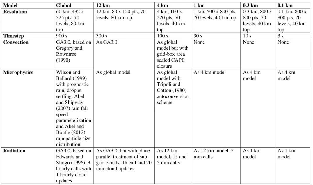
The configuration of the higher resolution domains follows the nested domains currently run over the UK for operational NWP (at least until 1-km resolution). Table I shows the main differences in their configuration from the global model. Some of the differences are required due to the resolution differences, whilst others are due to the latest physics developments not yet present in the higher resolution models. The limited-area domains use a rotated-pole coordinate system, placing the equator at the centre of the domain allowing an approximately uniform grid and a terrain-following hybrid-height vertical coordinate with Charney-Philips staggering (Arakawa and Konor, 1996).
The first nested domain has a horizontal grid-length of 12 km. The configuration of this nested domain is comparable to the North Atlantic and Europe model (NAE). The main difference from the global model is that the prognostic PC2 cloud scheme (Wilson et al., 2008) is replaced with the diagnostic scheme of Smith (1990). PC2 uses a prognostic representation of cloud fractions and liquid condensate by estimating their increments from each physical and dynamical process that is represented in the MetUM whereas the Smith (1990) scheme uses a prognostic variable characterising the total specific humidity and diagnoses the vapour and the liquid contents individually, whilst diagnosing a cloud fraction. This nested domain is reconfigured from the global model at 0100 UTC for both cases (i.e. T + 1) and thereafter is free-running throughout the case-study period, forced only at the boundaries by the global model.
The second nested domain has a horizontal grid length of 4 km. At this resolution, the convection is starting to be resolved on the model grid, so the convection scheme uses a
modified convective available potential energy closure (Lean et al., 2008). For this model, 70 levels are also employed in the vertical with the model lid placed at about 40 km, and the highest vertical resolution concentrated near the ground such that 23 levels span the lowest 2 km of the atmosphere. This resolution is reconfigured from the 12 km simulation at T + 1 (i.e. 0200 UTC) and is free-running thereafter, forced at the boundaries by the 12 km model. A third domain using 1 km grid-length is nested in the 4 km model. This model is comparable to the operational UKV forecast model and it runs without convection parameterization. The only other difference from the 4 km model is the horizontal diffusion which is based in this domain on the method of Smagorinsky (1963). Again, this model is re-configured at T + 1 from the 4 km domain (i.e. at 0300 UTC) and is free-running, forced at the boundaries by the 4 km model.
Finally, 0.3- and 0.1-km horizontal grid-length inner domains are used. As for the 1 km domain, no convection parameterization is used. The 0.3 km model is configured in a similar way to the 1 km model. The 0.1 km model is reconfigured at T + 1 from the 0.3 km domain (i.e. at 0400 UTC) and is free-running, forced at the boundaries by the 0.3 km model. For the different nested domains, the lateral boundary conditions are linearly interpolated in time between fields every hour for the 12- and 4-km models, and updated every 30 min for the others models.
2.2. The microphysics scheme
The MetUM cold microphysics scheme considers only one ice species as a prognostic variable (no graupel species) and no collision between ice and ice. This quantity is split by a diagnostic relationship, based upon both aircraft data (Houze et al., 1979; Field, 1999) and modelling data (Cardwell et al., 2002) into a large-ice (aggregate) and a small-ice (crystals) category which are then treated separately by the microphysical transfers before being
recombined after the transfers have been completed. Ice crystals can be formed via the homogeneous and heterogeneous nucleation processes. The homogeneous nucleation process assumes that all liquid water at temperatures less than -40ºC is instantaneously frozen to form ice crystals. The heterogeneous nucleation process is dependent on temperature, relative humidity and the mass of active nuclei (which is also temperature dependent). For ice to be produced by heterogeneous freezing, liquid water at temperatures colder than -10°C needs to be present. The description of the ice phase processes considered in this one-moment cold bulk scheme is detailed in Wilkinson (2011).
The standard warm microphysics scheme used in the MetUM is based on Wilson and Ballard (1999). However, extensive improvements have been made to this scheme in recent years (see Table I). Detailed descriptions of these changes can be found in Wilkinson et al. (2012) where the representation of drizzle and fog in the MetUM is examined. Here, the structure of the warm microphysics scheme is outlined. Water vapour is represented as a prognostic variable. Cloud liquid and rain are represented as single-moment bulk variables. Cloud and rain droplet numbers are diagnosed (i.e. not directly predict by the model) by the scheme and are not represented as prognostic variables. The prognostic rain formulation uses the Abel and Shipway (2007) rain fall speed parameterization and the Abel and Boutle (2012) rain particle size distribution.
The autoconversion scheme used in the MetUM is the same as used in Wilson and Ballard (1999) and is based on Tripoli and Cotton (1980) (referred hereafter by TC). The autoconversion scheme has two components: a cloud water mixing ratio threshold, below which there is no warm rain production via autoconversion, and the rate of change from cloud to rain above this threshold. The autoconversion rate, Raut, given by the Eq. (1), is dependent
on three model variables: air density, , the cloud liquid water mixing ratio, qcl, and the
, (1)
where Ec represents a collision/coalescence coefficient and is equal to 0.55 in default forecast
simulations. The parameter A is defined as,
, (2)
which has the numerical value 5907.24 at 0°C and g, and qw are, respectively, the
acceleration due to gravity, the dynamic viscosity of air and the water density.
The autoconversion threshold cloud water mixing ratio, qcl0, at which warm rain is presumed
to start in a given grid cell of the model, is given by:
, (3) where rcrit = 7 x 10⁻⁶ m.
The control MetUM simulations referred to later in the text assume a CDNC of 100 cm-3 over the ocean and 300 cm-3 over the land, to indicate that the land is more polluted. The control runs also use the same collision/coalescence coefficient (Ec = 0.55) used in the default
forecasting simulations.
Figure 2 shows the autoconversion threshold and rate used by the MetUM. Except at small CDNC, the autoconversion threshold is more sensitive to changes in CDNC than the autoconversion rate is. For example, a change in CDNC from 100 to 300 cm-3 makes precipitation formation more difficult by increasing the threshold water mixing ratio for autoconversion by a factor of 3.5 (i.e. precipitation requires 3.5 times more liquid water to start), while the autoconversion rate reduces by a factor of 1.4.
3. Simulation of two case-studies of UK convection
The case studies used were observed during the Convective Storm Initiation Project (CSIP, Browning et al., 2007) field campaign which took place in southern England in 2005. In order to characterize the effect of the character of the environment and the convection on the sensitivity to warm rain processes, two cases were selected with contrasting microphysical and dynamical characteristics.
The first case was observed on 4 July 2005 (IOP6). During the day, the CSIP area was under the influence of a strong north-westerly flow behind a low centred off the East Anglia region, on the west coast of England (see Browning and Morcrette, 2005). A cut-off low was over the area, characterised by low tropopause and cold air aloft producing a shallow boundary layer and low freezing level (see Figure 3). This led to modest CAPE (574 J kg-1), but with instability extending to about 7 km, and CIN was very small (2 J kg-1). The resulting moderately intense convective showers began in the morning and were observed until late afternoon (Figure 4).
The second case was observed on 13 July 2005 (IOP8). Two trailing cold fronts associated with a low pressure centred over Scandinavia brought cooler and cloudier conditions to Scotland and Northern Ireland. These fronts were weakening as they moved slowly southwards, advecting some mid- and upper-level cloud over the northern part of the CSIP domain. Convection developed over the CSIP area in association with the diurnal heating cycle. For this case, the simulated CAPE is equal to 435 J kg-1 and the CIN is equal to 20 J kg-1. A few brief light showers appeared mainly in the north-east of this area (Fig 4). Even farther to the north-east there were a few heavier showers, particularly towards the Cambridge area (see Bennett, 2007; Khodayar, 2009). During the afternoon, a sea-breeze penetrated inland from the south coast cutting off convection at the southern end of the band. Ahead of it, the atmosphere was warmer with a deeper boundary layer than the IOP6 (Figure 3), with weaker winds and less shear. These atmospheric conditions triggered the
development of a persistent convective storm a few kilometres to the north of London, which produced intense convective precipitation.
3.2 Control simulations
Figure 4 shows the comparison between the instantaneous precipitation fields obtained with the C-band rainfall radar retrievals from the UK radar network (called NIMROD) and the 1 km model for IOP6 at 1300 UTC and for IOP8 at 1600 UTC. These times are chosen because they correspond to the more intense phase of both systems of convection. Figure 4 shows that for IOP6 there was widespread precipitation over the North Sea, east of the UK. There were convective showers along the west coast, with lines of showers running northwest to south east across the south of the UK. These showers are likely tied to both convergence lines driven by coastlines and orography and an upper-level PV anomaly (Browning and Morcrette, 2005). The model produces similar north-west-southeast lines of showers over the southern UK (with a line extending inland from northwest Wales), but exhibits larger errors further north, likely due to errors in the upper-level PV (Browning and Morcrette, 2005). IOP 8 is characterized by a persistent storm in south east England (a few kilometres to the north of London) and a line of showers running southwest from this (Figure 4), likely associated with sea-breeze convergence (Browning and Morcrette, 2005). The 1-km model captures this line of showers, with heavier rain in the northeast, but over-predicting the rainfall intensity in the southwest. The finer model grid spacing compared to the 5-km radar grid may contribute to this difference. Nevertheless, this difference is slightly reduced when model results are smoothed to 5 km grid spacing. For both IOP6 and IOP8, the model captures the location and timing of the precipitation well enough for us to proceed with a sensitivity study, focused on southern England (the 333 m domain, Figure 3).
Figures 5 and 6 respectively show that the organisation of the convection is similar at 333 m and 100 m grid-spacing for IOP6, whereas for IOP8 the 100 m grid-spacing gives narrower showers. Moreover, between 1 km and 333-m resolution, both IOP6 and IOP8 have a change in the locations of the heaviest precipitation. The finer scale representation of the convection can cause this spatial shift. In the lower resolution model (1-km model) the convection is permitted but not well resolved, whereas it is better resolved in the finest one (333-m model). This difference in the ability to resolve the cloud will lead to differences in the feedback onto the thermodynamics and dynamics of subsequent cloud and precipitation. Nevertheless, in this work, our subsequent results on sensitivities to CDNC are robust to the grid-spacing used in each case for grid-spacing less than 4 km (the same might not be true in a model where resolved vertical winds affect aerosol activation).
4. Sensitivity to warm rain formation
In order to study the importance of variations in the threshold for and rate of warm-rain formation by autoconversion, several sensitivity studies were performed varying the CDNC parameter in the autoconversion scheme (Eq. (1)) to “polluted” (nd = 900 cm-3 over land) and
“clean” (nd = 100 cm-3 over land). Hereafter, only the model results obtained with the 333 m
horizontal grid spacing are presented, but, the tendencies are similar for other horizontal resolutions used such as 4-, 1- and 0.1-km.
Figure 7 shows probability density functions (PDFs) of the surface rain rate multiplied by the corresponding rain rates for both cases studied for the entire lifetime systems. This is the first moment of the precipitation distribution. In this way the area under the curve represents total rain rate. In both cases the lowest precipitation rates are more numerous than the highest ones and contribute more to the rainfall totals.
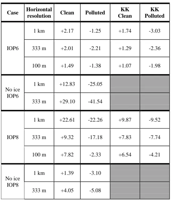
For IOP6, Figure 7a shows that the surface rain rates are similar whatever the CDNC, although the clean simulations give slightly more rain in the 2.5-8 mm h-1 range. Table II shows that the relative difference in the total rain rate between the default and each sensitivity simulations for the 333-m modelled results is very small whatever the horizontal grid spacing used, since the maximum difference is only about -2%. The results are perhaps surprising; a modification by a factor of 9 in the cloud droplet concentration has no significant effect on the surface precipitation field in this case where the liquid water path (LWP) is quite high (up to 423 g m-2) but less important than the Ice Water Path (IWP) (up to 3231 g m-2). In the larger grid spacing simulation (1 km) the LWP is approximately 2.3 times larger than in the 333 m simulations. Nevertheless, some studies, such as Seifert et al. (2012), have shown that high LWP may result in little sensitivity of precipitation to aerosol number concentration. In the IOP8 case (Figure 7b) the changes in CDNC induce more significant modifications in the surface precipitation rates. The increase in the CDNC causes a decrease of the surface precipitation rates which is more important for the lowest rain rates. The highest rain rates seem rather similar whatever the cloud droplet concentration used. Table II shows that an increase in the CDNC by a factor of 3 causes a decrease of 17% in the total precipitation for the polluted environment (considering the 333-m horizontal grid spacing). Table II also shows that the tendency is similar whatever the resolution but the relative differences in the precipitation rate are more important in the 1 km model simulations. The representation of the convection at different resolutions can account for these different responses of precipitation rate to changes in droplet concentrations: e.g. vertical wind speeds attain highest values (twice as high, i.e 14 m s-1) in the simulations using fine resolution (not shown), which then can impact the LWP.
Figure 8 shows the PDFs of the surface rain rate in simulations where the autoconversion parameterization of TC is replaced by the approach of Khairoutdinov and Kogan (2000)
(referred hereafter by KK) (see Boutle et al. (2013) for more details). This KK autoconversion scheme is used in many global and operational models such as e.g. the NCAR CAM global model (Gettelman et al., 2013). When the KK autoconversion is used IOP6 is still insensitive whereas IOP8 shows sensitivity to changes in CDNC, however, the response of IOP8 appears much weaker with the KK scheme (also visible in Table II). This small response is due to the fact that the KK scheme produces less rain than the default autoconversion scheme (Figures 7 and 8). This trend is consistent with the conclusions of Wood (2005) and may be due to the fact that the KK scheme was developed in stratocumulus clouds where the associated precipitation is less intense than in convective clouds. However, the changes in warm rain production are dependent on the cloud microphysics and dynamics of both cases since the contrasted tendency between both cases remains the same whatever the autoconversion scheme used.
4.1 Impacts of changes to warm rain on cloud dynamics
In order to explain the contrasting behaviour of the two cases, the dynamical and microphysical properties that influence the evolution of the cloud systems in the different simulated environments are now analysed. These simulations are done with the default TC autoconversion scheme and not with the KK scheme.
Figure 9 shows the temporal evolution of the variance of the vertical wind speed at the cloud base (i.e. only cloud regions where qc > 0.01 g kg-1 are sampled) for both CSIP cases.
Modifying the CDNC has no strong influence on the dynamical development of the two convective cases since the variation of the vertical wind variance is very small for IOP6 case while there are no relevant changes for IOP8. Indeed, the overall shapes of the hourly PDFs of the vertical wind speeds obtained for IOP8 remain similar whatever the cloud droplet concentrations. As regards the hourly PDFs of the vertical wind speeds for IOP6, it seems
that the small variation of the variance is mainly due to the frequencies of the strongest updrafts. For example, at 1300 UTC, the maximum vertical wind speed in the clean test is 7.5 m s-1 whereas it is 5.5 m s-1 in the polluted and default tests. However, the frequency for these maximal values is 5 orders of magnitude lower than the most common values.
4.2 Impacts of changes to warm rain on cloud microphysics
As shown in Figure 3 and explained in Section 3, the two cases have contrasted synoptic and thermodynamic conditions. IOP6 is colder than IOP8 since the 0°C level is lower and very close to the lifting condensation level (LCL). Indeed, the 0°C and the LCL are respectively situated at 800 hPa and 830 hPa in IOP6 and 750 hPa and 800 hPa in IOP8 (Figure 3). In order to understand if the ice phase can explain the lack of sensitivity to the CDNC in IOP6, simulations where the ice phase is switched off were performed. Figure 10 shows the PDF of the precipitation rate multiplied by the precipitation rate for both cases (the same representation as Figure 7). The grey lines show the default simulations for the IOP6 and IOP8 cases (same as the black solid lines in Figure 7) and the black solid lines correspond to the default case when the ice phase is switched off. The precipitation rate decreases significantly when no ice is present in the IOP6 simulations; this is consistent with more efficient formation of precipitation due to ice (Pruppacher and Klett, 1997). The same tendency is visible for the IOP8 simulations even if the decrease in the precipitation rate is weaker in this case (- 3%). Considering the same sensitivity studies as in Section 4, Figure 10 shows that the IOP6 convective system becomes sensitive to the CDNC when the ice phase is switched off (dashed and dotted lines): for example, focussing on the 333 m model results and considering the IOP6 clean simulations, the relative difference in the precipitation rate with the default case increases from +2% to +29% (Table II). For IOP8, the no-ice run shows that ice is not playing such a strong role in this case, since the PDF of the precipitation rate
does not change when the ice phase is switched off and the sensitivity to CDNC is maintained. This initial investigation shows that the mechanisms of the ice phase plays a role in the contrasting behaviour of the two mixed-phase convective systems studied.
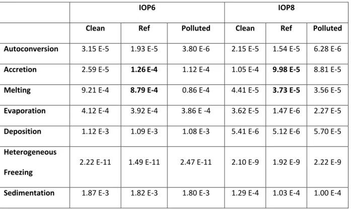
Figure 11 shows the domain-averaged vertical profiles of the mixing ratios of the cloud liquid phase (black lines), the cloud ice phase (dark grey lines) and rain (light grey) for both cases (where the ice phase is not switched off) and default (asterisks), clean (diamonds) and polluted (squares) environments. The averages are obtained over the 333-m model domain and over the lifetime of each convective system. Figures 11a and b show that the default IOP8 cloud is deeper with a higher altitude cloud base than the IOP6 system. Figure 11a shows that the different sensitivity studies on the CDNC do not influence the precipitation and only slightly impact the different cloud water fields of the IOP6 case. The mean rates of cloud processes (obtained using the same averaging approach as for Figure 11) directly involved in the rain formation for the IOP6 case are represented in the Figure 12. For IOP6, the autoconversion and the rain evaporation rates are sensitive to drop number while accretion rate is nearly independent of the cloud drop number. The melting process is independent of the CDNC. However, the slight changes in the autoconversion and the evaporation rates have no influence on the rain production since for rain production the melting process is more than one order of magnitude more important (see Table III). Therefore, the lack of sensitivity in the surface precipitation of the IOP6 case is due to the fact that the rain production is dominated by the ice phase and the ice processes are not sensitive to the change in CDNC, since the warm rain process removes very little water that would otherwise form ice in these cold clouds (as discussed for example in Van den Heever et al., 2006; Rosenfeld and Khain, 2008; Khain, 2009).
Figure 11b illustrates the mean vertical profiles of the mixing ratios of the cloud water phases and rain for IOP8. Figure 13 represents the rate of the main cloud processes involve in the
warm rain formation using the same representation as in Figure 12. Figure 11b shows that an increase in the CDNC produces an increase of the cloud liquid mixing ratio whereas the rain mixing ratio decreases. This tendency is comparable with the work of Planche et al. (2010) on a warm shallow convective system where the increase in the aerosol number concentration produces a decrease in the precipitation accumulation. Figure 11b also shows that an increase in the CDNC induces a decrease of the cloud ice mixing ratio. This result is opposite to the Rosenfeld et al. (2008) convective invigoration hypothesis where it is suggested that an increase in CDNC produces less warm rain but more ice particles. However, it should be borne in mind that the microphysics used here has no explicit dependence on aerosol number and so changes to the ice phase will only be linked to changes in cloud dynamical and thermodynamical evolution. Note that the changes in the cloud mixing ratios are less significant than the sensitivity of the precipitation at the ground. However, if the average of the mixing ratios conditionally samples only the cloudy columns where the surface precipitation is greater than zero, the polluted environment gives results more comparable to the proposal of Rosenfeld et al. (2008) since there is more cloud ice and more rain than the default case at low levels (not shown). Therefore in the polluted run, the rainy columns are icier, but they are fewer than in the clean study (consistent with Figure 7b). The increase in cloud-ice does not lead to increased rain to compensate for the loss of warm rain production in the polluted case. Figure 13 shows that the changes in the CDNC influences, to varying degrees, all of the processes involved in the rain formation of the IOP8 case. The change in the CDNC mainly influences the warm rain processes such as the autoconversion of cloud water to rainwater and the rain evaporation. The variation in the accretion process is nevertheless the most important term (Table III). The domain-average of the mixing ratios confirms that warm rain dominated columns are more numerous than ice process dominated columns. The freezing rate is slightly more important in the polluted case than in the default
case, but with 5 orders of magnitude less important than e.g. the accretion or the melting rates. The heterogeneous freezing is visible between approx. 6 and 8 km height due to the presence of a small amount of cloud water, a high amount of cloud ice and temperatures colder than -10°C. Note that the vertically integrated melting rate is 2.5 times lower than vertically integrated accretion and the vertically integrated ice sedimentation rate of the polluted case is 1.25 times bigger for the default case. The deposition of vapour on to ice is less important in the polluted case than in the default case. This reduction in the deposition rate is due to a reduction in the relative humidity with respect to the ice.
Regarding both cases, it seems that the integral of the melting rate and accretion rate indicate whether the cloud will be sensitive to CDNC for this model with very simplified microphysics.
5. Conclusions
In this study, the impacts of changing warm-rain production by CDNC on UK convection in convection-permitting and convection-resolving simulations using an operational NWP model are analysed. Two mixed-phase convective summertime systems with contrasting characteristics observed during the CSIP campaign in southern England in 2005 have been simulated using the Met Office Unified Model. Although sensitivity to warm rain production has been investigated for many cases, there are very few such studies for moist convection in the mid-latitude maritime environment of the UK. The first case (IOP6) is characterised by moderately intense convective showers forming throughout the day in a north-westerly airstream below an upper-level PV anomaly, with a shallow boundary layer and low freezing level. The second case (IOP8) is warmer with a deeper boundary layer with weaker winds and less shear, and is characterised by isolate convective cells, with one persistent stronger storm. In order to simulate both cases at very high resolution, a suite of one-way nested
models was used with grid lengths of 12, 4, 1, 0.333 and 0.1 km. The simulations reproduce the convective showers observed in the area of interest, although the model also generates spurious precipitation outside of this area in IOP6.
In order to evaluate the impact of CCN on the precipitation associated with mixed-phase convective systems in a NWP model, the role of the CDNC (that is not represented expliciltly in this model) via its impact on the autoconversion process (that is represented explciltly in this model) on the cloud evolution and precipitation formation is investigated. The influence on precipitation formation is very different between the two cases: the IOP6 case is almost insensitive to large changes in CDNC, while in the IOP8 case a change of a factor of 3 in assumed CDNC affects total precipitation by a maximum of ~17%. In both cases the sensitivities to CDNC are similar at all grid-spacings lower or equal to 1 km (although vertical velocities and cloud organisation are more sensitive to grid-spacing). The contrasting sensitivities of the two cases are induced by the contrasting role of the ice phase proportion in each case. Due to the dominance of the ice phase in IOP6, the impact of the CDNC changes on rain processes and then on the surface precipitation rain rates is small. In contrast, for the IOP8 mixed-phase cloud system, where the cloud ice phase is less important than the cloud liquid phase, an increase in the CDNC produces a decrease in the warm rain production. The frequency of light rain (likely from warm processes) is reduced, while the frequency of heavy rain (likely from ice) is largely unaffected. Decreased warm rain leads to a reduction in overall rain, and unlike many previous studies (Seifert and Beheng, 2006b; Morrison and Grabowski, 2011) there is no evidence of increased ice production to compensate for this decrease. This study shows a non-linear response of the mixed-phase convective systems to the change of the efficiency of warm rain production. It is also noticeable that the sensitivities of surface precipitation to variations in CDNC are only half as important as changes are the grid-spacing from 1 km to 100 m. This highlights the importance of resolving updraughts and
mixing. Some other studies show small precipitation sensitivity to CDNC or aerosols. Seifert et al. (2012), who showed little effect of CCN or IN on surface precipitation but a strong effect on in-cloud properties, concluded that cloud systems are buffered systems (Stevens and Feingold, 2009) because a microphysical cloud process which becomes more efficient or a different dynamical evolution of the system can compensate the aerosol effect on precipitation. Khain (2009) also showed how the short distance from the Lifting Condensation Level to freezing level reduces sensitivity to CCN.
In this study, we used a single-moment bulk microphysics. Such microphysics schemes are simple but are generally used in global and regional operational NWP models. The single-moment microphysics schemes have some limitations in the representation of the microphysics processes such as evaporation or sedimentation that are important in the evolution of precipitation and are sensitive to the hydrometeor size distribution. For example, Dawson et al. (2010) showed that, during sedimentation, the size distribution can become narrower from size sorting, which is not permitted in single-moment schemes because a single fall speed for the predicted moment for a hydrometeor category is used. To confirm and/or extend our findings on the impacts of changing warm-rain production in an operational NWP model, where the effects of variations in aerosol are introduced by simply changing CDNC, further simulation analyses using a more sophisticated multi-moment bulk microphysics scheme are necessary (e.g. Shipway and Hill, 2012, among others).
Acknowledgement
The lead author would like to thank the two anonymous reviewers for their precise and constructive comments which have significantly contributed to the improvement of the article. The lead author also thanks Jonathan Wilkinson, Stuart Webster and Ian Boutle for, respectively, their help in explaining the UM microphysics scheme options, debugging the
nesting suite procedure and providing the branch permitting the installation of the KK scheme in the UM_7.7.
The AeroSol Cloud Interactions project was made possible through the financial support of the Leeds-Met Office Academic Partnership. We acknowledge use of MONSooN system, a collaborative facility supplied under the Joint Weather and Climate Research Programme, which is a strategic partnership between the Met Office and the Natural Environment Research Council.
References
Abel SJ, Boutle IA. 2012. An improved representation of the rain size spectra for single-moment microphysics schemes. Quart. J. Roy. Meteor. Soc. 138: 2151-2162. DOI: 10.1002/qj.1949.
Abel SJ, Shipway BJ. 2007. A comparison of cloud-resolving model simulations of trade wind cumulus with aircraft observations taken during RICO. Quart. J. Roy. Meteor. Soc. 133: 781-794. DOI: 10.1002/qj.55.
Arakawa A, Konor CS. 1996. Vertical differencing of the primitive equations based on the Charney-Phillips grid in Hybrid -p coordinates. Mon Wea. Rev. 124: 511-528.
Beheng KD. 1994. A parameterization of warm cloud microphysical conversion processes. Atmos. Res. 33: 193-206. DOI: 10.1016/0169-8095(94)90020-5.
Bennett LJ. 2007. Observations of boundary-layer development and initiation of precipitating convection. PhD thesis. University of Leeds, UK. 233pp.
Berry EX. 1967. Cloud droplet growth by collection. J. Atmos. Sci. 24: 688-701. DOI: 10.1175/1520-0469(1967)024<0688;CDGBC>2.0.CO;2.
Boutle IA, Abel SJ, Hill PG, Morcrette CJ. 2013. Spatial variability of liquid cloud and rain: observations and microphysical effects. Quart. J. Roy. Meteor. Soc. DOI: 10.1002/qj.2140. Boutle IA, Morcrette CJ. 2010. Parametrization of area cloud fraction. Atmos. Sci. Lett. 11:
283-289.
Browning K, Morcrette C. 2005. A summary of the Convective Storm Initiation Project Intense Observation Periods (CSIP IOPs). Forecasting Technical Report No. 474, available from http://www.metoffice.gov.uk
Browning KA, Blyth AM, Clark PA, Corsmeier U, Morcrette CJ, Agnew JL, Ballard SP, Bamber D, Barthlott C, Bennett LJ, Beswick KM, Bitter M, Bozier KE, Brooks BJ, Collier CG, Davies F, Deny B, Dixon MA, Feuerle T, Forbes RM, Gaffard C, Gray MD, Hankers
R, Hewison TJ, Kalthoff N, Khodayar S, Kohler M, Kottmeier C, Kraut S, Kunz M, Ladd DN, Lean HW, Lenfant J, Li Z, Marsham J, Mcgregor J, Mobbs SD, Nicol J, Norton E, Parker DJ, Perry F, Ramatschi M, Ricketts HMA, Roberts NM, Russell A, Schulz H, Slack EC, Vaughan G, Waight J, Wareing DP, Watson RJ, Webb AR, Wieser A. 2007. The Convective Storm Initiation Project. Bull. Am. Meteorol. Soc. 88: 1939-1955. DOI: 10.1175/BAMS-88-12-1939
Cardwell JR, Choularton TW, Wilson DR, Kershaw R. 2002. Use of an explicit model of the microphysics of precipitating stratiform cloud to test a bulk microphysics scheme. Quart. J. Roy. Meteor. Soc. 128: 573-592.
Cui Z, Davies S, Carslaw KS, Blyth AM, Blyth AM. 2010. The response of precipitation to aerosol through riming and melting in deep convective clouds. Atmos. Chem. Phys. Disc., 10: 29007-29050. doi: 10.5194/acpd-10-29007-2010.
Cui Z, Carslaw KS, Davies S, Yin Y. 2006. A numerical study of aerosol effects on the dynamics and microphysics of a deep convective cloud in a continental environmental. J. Geophys. Res. 111: D05201. doi: 10.1029/2005JD005981.
Cullen MJP, Davies T, Mawson MH, James JA, Coulter SC, Malcolm A. 1997. An overview of numerical methods for the next generation UK NWP and climate model. Numerical Methods in Atmospheric and Ocean Modelling: The André J. Robert Memorial Volume, Lin CA, Laprise R, Ritchie H, Eds., Canadian Meteorological and Oceanographic Society, 425-444.
Davies T, Cullen MJP, Malcolm A, Mawson MH, Staniforth A, White AA, Wood N. 2005. A new dynamical core for the Met Office’s global and regional modelling of the atmosphere. Quart. J. Roy., Meteor. Soc. 131: 1759-1782. DOI: 10.1256/qj.04.101.
Dawson DT, Xue M, Milbrandt JA, Yau MK. 2010. Comparison of evaporation and cold pool development between single-moment and multimoment bulk microphysics schemes in idealized simulations of tornadic thunderstorms. Mon. Wea. Rev. 138: 1152-1171. Devine GM, Carslaw KS, Parker DJ, Petch JC. 2006. The influence of subgrid surface-layer
variability on the vertical transport of a chemical species in a convective environment. Geophys. Res. Lett. 33: L15807. DOI: 0.1029/2006GL025986.
Edwards JM, Slingo A. 1996. Studies with flexible new radiation code. I. Choosing a configuration for large-scale model. Quart. J. Roy. Meteor. Soc. 122: 689-719.
Essery R, Best M, Cox P. 2001. MOSES 2.2 Tech. Doc. Hadley Centre Tech. Rep. 30, Met Office Hadley Centre, 30 pp.
Field PR. 1999. Aircraft observations of ice crystal evolution in an altostratus cloud. J. Atmos. Sci. 56: 1925-1941.
Gettelman A, Morrison H, Terai CR, Wood R. 2013. Microphysical process rates and global aerosol-cloud interactions. Atmos. Chem. Phys. 13: 9855-9867.
Grabowski WW. 2006. Indirect impact of atmospheric aerosols in idealized simulations of convective-radiative quasi equilibrium. J. Climate. 19: 4664-4682. DOI: 10.1175/JCLI3857.1.
Graf HF. 2004. The complex interaction of aerosols and clouds. Science. 303: 1309-1311. DOI: 10.1126/science.1094411.
Gregory D, Rowntree PR. 1990. A mass flux convection scheme with representation of cloud ensemble characteristics and stability-dependent closure. Mon. Wea. Rev. 118: 1483-1506. DOI: 10.1175/1520-0493(1990)118<1483:AMFCSW>2.0.CO;2.
Houze RA, Hobbs PV, Herzegh PH, Parsons DB. 1979. Size distributions of precipitation particles in frontal clouds. J. Atmos. Sci. 36: 156-162.
Kessler E. 1969. On the distribution and continuity of water substance in atmospheric circulation. Meteor. Monogr. 32: 84 pp. Amer. Meteor. Soc., Boston, Mass.
Khain AP. 2009. Notes on state-of-the-art investigations of aerosol effects on precipitation: a critical review. Environ. Res. Lett. 4: 015004. DOI: 10.1088/1748-9326/4/1/015004. Khain A, Pokrovsky A, Pinsky M, Seifert A, Phillips V. 2004. Simulation of Effects of
Atmospheric Aerosols on Deep Turbulent Convective Clouds Using a Spectral Microphysics Mixed-Phase Cumulus Cloud Model. Part I: Model Description and Possible Applications. J. Atmos. Sci. 61: 2963-2982. DOI: http://dx.doi.org/10.1175/JAS-3350.1 Khairoutdinov M, Kogan Y. 2000. A new cloud physics parameterization in a large-eddy
simulation model of marine stratocumulus. Mon Wea. Rev. 128: 229-243. DOI: 10.1175/1520-0493(2000)128<0229:ANCPPI>2.0CO;2.
Khodayar S. 2009. High-resolution analysis of the initiation of the deep convection forced by boundary-layer processes. PhD thesis. University of Karlsruhe, Germany. 173pp.Lean HW, Clark PA, Dixon M, Roberts NM, Fitch A, Forbes R, Halliwell C. 2008. Characteristics of high-resolution versions of the Met Office Unified Model for forecasting convection over the UK. Mon. Wea. Rev. 136: 3408-3424.
Lee SS, Donner LJ, Phillips VTJ, Ming Y. 2008. The dependence of aerosol effects on clouds and precipitation on cloud-system organization, shear and stability. J. Geophys. Res. 113: D16202. doi: 10.1029/2007JD009224.
Lee SS, Feingold G. 2013. Aerosol effects on the cloud-field properties of tropical convective clouds. Atmos. Chem. Phys. Discuss. 13: 2997-3029. DOI: 10.5194/acpd-13-2997-2013. Levin Z, Cotton WR. 2009. Aerosol Pollution Impact on Precipitation, a Scientific Review.
Lock AP, Brown AR, Bush MR, Martin GM, Smith RNB. 2000. A new boundary layer mixing scheme. Part I: Scheme description and single-column model tests. Mon. Wea. Rev., 128: 3187-3199. DOI: 10.1175/1520-0493(2000)128<3187:ANBLMS>2.0.CO;2. Lohmann U, Feichter J. 2005. Global indirect aerosol effects: a review. Atmos. Chem. Phys.
5: 715-737. DOI: 10.5194/acp-5-715-2005.
Milbrandt J, McTaggart-Cowan R. 2010. Sedimentation-induced errors in bulk microphysics schemes. J. Atmos. Sci. 67: 3931-3948.
Morrison H, Grabowski WW. 2011. Cloud-system resolving model simulations of aerosol indirect effects on tropical deep convection and its thermodynamic environment. Atmos. Chem. Phys. 11: 10503-10523.
Morrison H, Thompson G, Tatarskii V. 2009. Impact of cloud microphysics on the development of trailing stratiform precipitation in a simulated squall line: Comparison of one- and two-moment schemes. J. Atmos. Sci. 137: 991-1007.
Planche C, Wobrock W, Flossmann AI, Tridon F, Van Baelen J, Pointin Y, Hagen M. 2010. The influence of aerosol particle number and hygroscopicity on the evolution of convective cloud systems and their precipitation: A numerical study based on the COPS observations on 12 August 2007. Atmos. Res. 98: 40-56. DOI: 10.1016/j.atmosres.2010.05.003.
Pruppacher HR, Klett JD. 1997. Microphysics of clouds and precipitation. Kluwer Academic Publishers, Dordrecht, the Netherlands, 954pp.
Rosenfeld D, Khain A. 2008. Anthropogenic aerosol invigorating hail. Proc. Int. Conf. on Clouds and Precipitation (Cancun, July 2008).
Rosenfeld D, Lohmann U, Raga GB, O’Dowd CD, Kulmala M, Fuzzi S, Reissell A, Andreae MO. 2008. Flood or Drought: How Do Aerosols Affect Precipitation? Science. 321: 1309-1313. DOI: 10.1126/science.1160606.
Seifert A, Beheng KD. 2006a. A two-moment cloud microphysics parameterization for mixed-phase clouds. Part 1: Model description. Meteorol. Atmos. Phys. 92: 45-66. DOI: 10.1007/s00703-005-0112-4.
Seifert A, Beheng KD. 2006b. A two-moment cloud microphysics parameterization for mixed-phase clouds. Part 2: Maritime vs. continental deep convective storms. Meteorol. Atmos. Phys. 92: 67-82. DOI: 10.1007/s00703-005-0113-3.
Seifert A, Köhler C, Beheng KD. 2012. Aerosol-cloud-precipitation effects over Germany as simulated by a convective-scale numerical weather prediction model. Atmos. Chem. Phys. 12: 709-725.
Shipway BJ, Hill AA. 2012. Diagnosis of systematic differences between multiple parameterizations of warm rain microphysics using a kinematic framework. Quart. J. Roy. Meteor. Soc. 138: 2196-2211. DOI: 10.1002/qj.1913.
Smagorinsky J. 1963. General circulation experiments with the primitive equations. Part I: the basic experiment. Mon. Wea. Rev. 91: 99-164.
Smith RNB. 1990. A scheme for predicting layer clouds and their water content in a general circulation model. Quart. J. Roy. Meteor. Soc. 116: 435-460. DOI: 10.1002/qj.49711649210.
Solomon S, Qin D, Manning M, Alley RB, Berntsen T, Bindoff NL, Chen Z, Chidthaisong A, Gregory A, Hegerl GC, Heimann M, Hewitson B, Hoskins BJ, Joos F, Jouzel J, Kattsov V, Lohmann U, Matsuno T, Molina M, Nicholls N, Overpeck J, Raga G, Ramaswamy V, Ren J, Rusticucci M, Somerville R, Stocker TF, Whetton P, Wood RA, Wratt D. 2007. Technical summary. In: Climate change 2007: The physical science basis. Contribution of working group I to the Fourth Assessment Report of the Intergovernmental Panel on Climate Change. Cambridge University Press, Cambridge, United Kingdom and New York, NY, USA.
Stevens B, Feingold G. 2009. Untangling aerosol effects on clouds and precipitation in a buffered system. Nature. 461: 607-613. DOI: 10.1038/nature08281.
Tao WK, Chen JP, Li Z, Wang C, Zhang C. 2012. Impact of aerosols on convective clouds and precipitation. Rev. Geophys. 50: RG2001. DOI: 10.1029/2011RG000369
Tripoli GJ, Cotton WR. 1980. A numerical investigation of several factors contributing to the observed variable intensity of deep convection over Florida. J. Appl. Meteorol. 19: 1037-1063.
Van den Heever SC, Carrio GG, Cotton WR, Demott PJ and Prenni AJ. 2006. Impacts of nucleating aerosol on Florida storms. Part I: mesoscale simulations. J. Atmos. Sci. 63: 1752–1775.
Walters DN, Best MJ, Bushell AC, Copsey D, Edwards JM, Falloon PD, Harris CM, Lock AP, Manners JC, Morcrette CJ, Roberts MJ, Stratton RA, Webster S, Wilkinson JM, Willett MR, Boutle IA, Earnshaw PD, Hill PG, MacLachlan C, Martin GM, Moufouma-Okia W, Palmer MD, Petch JC, Rooney GG, Scaife AA, Williams KD. 2011. The Met Office Unifed Model Global Atmosphere 3.0/3.1 and JULES Global Land 3.0/3.1 configurations. Geosci. Model. Dev. 4: 919-941.
Webster S, Uddstorm M, Oliver H, Vosper S. 2008. A high-resolution modelling case study of a severe weather event over New Zealand. Atmos. Sci. Let. 9: 119-128. DOI: 10.1002/asl.172.
Wilkinson J. 2011. The large-scale precipitation parameterization scheme. Met Office internal report. 52 pp.
Wilkinson JM, Porson ANF, Bornemann FJ, Weeks M, Field PR, Lock AP. 2012. Improved microphysical parameterization of drizzle and fog for operational forecasting using the Met Office Unified Model. Quart. J. Roy. Meteor. Soc. DOI: 10.1002/qj.1975.
Wilson DR, Ballard SP. 1999. A microphysically based precipitation scheme for the UK Meteorological Office Unified Model. Quart. J. Roy. Meteor. Soc. 125: 1607-1636. DOI: 10.1256/smsqj.55706.
Wilson DR, Bushell AC, Kerr-Munslow AM, Price JD, Morcrette CJ. 2008. PC2: a prognostic cloud fraction and condensation scheme. I: Scheme description. Quart. J. Roy. Meteor. Soc. 134: 2093-2107.
Wood R. 2005. Drizzle in stratiform boundary layer clouds. Part II: Microphysical aspects. J. Atmos. Sci. 62: 3034-3050.
Xue H, Feingold G, Stevens B. 2008. Aerosol effects on cloud, precipitation, and the organization of shallow convection. J. Atmos. Sci. 65: 392-406. DOI: 10.1175/2007JAS2428.1.
Yin Y, Carslaw K, Feingold G. 2005. Vertical transport and processing of aerosols in a mixed-phase convective cloud and the feedback on cloud development. Quart. J. Roy. Meteor. Soc. 131: 221-245. DOI: 10.1256/gj.030186.
Tables
Table I: Table showing the differences between different resolution models.
Table II: Relative difference (in %) between the total surface rain rate in the default case and obtained with the different sensitivity studies on the cloud droplet concentration. The total surface rain rates obtained for each horizontal resolution are computed over the entire lifetime of the convective system and over all the grid points of the associated domain (see Figure 1). The columns intituled KK represent the results obtained using the autoconversion scheme of Khairoutdinov and Kogan (2000) instead of the Tripoli and Cotton (1980) scheme. Table III: Total (sum over the vertical layers) of the mean rate of the different microphysical processes involved in the precipitation formation (in g kg-1 s-1). The total values are obtained for the 333-m simulations for both cases.
Table I 1 2 Model Global 12 km 4 km 1 km 0.3 km 0.1 km Resolution 60 km, 432 x 325 pts, 70 levels, 80 km top 12 km, 80 x 120 pts, 70 levels, 80 km top 4 km, 160 x 220 pts, 70 levels, 40 km top 1 km, 500 x 800 pts, 70 levels, 40 km top 0.3 km, 800 x 800 pts, 70 levels, 40 km top 0.1 km, 800 x 800 pts, 70 levels, 40 km top Timestep 900 s 300 s 100 s 30 s 10 s 3 s
Convection GA3.0, based on
Gregory and Rowntree (1990)
As GA3.0 As global
model but with grid-box area scaled CAPE closure
None None None
Microphysics Wilson and
Ballard (1999) with prognostic rain, droplet settling, Abel and Shipway (2007) rain fall speed parameterization and Abel and Boutle (2012) rain particle size distribution
As global model As global model with Tripoli and Cotton (1980) autoconversion scheme As 4 km model As 4 km model As 4 km model
Radiation GA3.0, based on
Edwards and Slingo (1996). 3 hourly calls with 1 hourly cloud
As GA3.0, but with plane-parallel treatment of sub-grid clouds. 1h call and 20 min cloud updates
As 12 km model. 15 and 5 min calls As 12 km model. 5 min calls As 1 km model As 1 km model
Cloud PC2 (Wilson et al., 2008)
Smith (1990) with cloud area parameterization discussed in Boutle and Morcrette (2010). RHcrit = 0.8 above 900m, linearly increasing to 0.91 at surface As 12 km model As 12 km model Smith (1990). RHcrit = 0.97 at each level Smith (1990). RHcrit = 0.99 at each level
Horizontal diffusion None None 2
with fixed K = 8.5 x 10³ Smagorinsky (1963) type scheme As 1 km model As 1 km model Vertical diffusion GA3.0, based on
Lock et al. (2000)
Table II
Case Horizontal
resolution Clean Polluted
KK Clean KK Polluted IOP6 1 km +2.17 -1.25 +1.74 -3.03 333 m +2.01 -2.21 +1.29 -2.36 100 m +1.49 -1.38 +1.07 -1.98 No ice IOP6 1 km +12.83 -25.05 333 m +29.10 -41.54 IOP8 1 km +22.61 -22.26 +9.87 -9.52 333 m +9.32 -17.18 +7.83 -7.74 100 m +7.82 -2.33 +6.54 -4.21 No ice IOP8 1 km +1.39 -3.10 333 m +4.05 -5.08
Table III
IOP6 IOP8
Clean Ref Polluted Clean Ref Polluted
Autoconversion 3.15 E-5 1.93 E-5 3.80 E-6 2.15 E-5 1.54 E-5 6.28 E-6
Accretion 2.59 E-5 1.26E-4 1.12 E-4 1.05 E-4 9.98 E-5 8.81 E-5
Melting 9.21 E-4 8.79 E-4 0.86 E-4 4.41 E-5 3.73 E-5 3.56 E-5
Evaporation 4.12 E-4 3.92 E-4 3.86 E -4 3.62 E-5 1.47 E-6 2.27 E-5
Deposition 1.12 E-3 1.09 E-3 1.08 E-3 5.41 E-6 5.12 E-6 5.70 E-5
Heterogeneous Freezing
2.22 E-11 1.49 E-11 2.47 E-11 2.10 E-9 1.92 E-9 2.22 E-9
Figures
Figure 1: Domains from n1 to n5 used for the 12-, 4-, 1-, 0.3- and 0.1-km models. The continuous and dashed lines represent the domain used respectively for the IOP8 and IOP6 case.
Figure 2: Autoconversion threshold (a) and rate (b) in the MetUM as a function of cloud droplet number concentration. The default simulation considers same values than forecast runs, i.e. Ec = 0.55, nd = 100 cm-3 over sea grid points and nd = 300 cm-3 over land grid
points.
Figure 3: Tephigram of the mean vertical profile of the simulated dew point temperature (dashed line) and temperature (solid line) for both cases: IOP6 (in grey) and IOP8 (in black) for the 333m-model.
Figure 4: Comparison between the precipitation fields obtained with the radar observations of the NIMROD network and the 1 km model for the IOP6 at 1300 UTC and for the IOP8 at 1600 UTC.
Figure 5: Instantaneous rainfall rates of the CSIP IOP6 case over the 100-m model area and at 1300 UTC for runs which start at 0000 UTC: (a) 4-km model, (b) 1-km model, (c) 333-m model, (d) 100-m model.
Figure 6: As Figure 5, but at 1600 UTC and for CSIP IOP8 case.
Figure 7: Probability density function of the precipitation rate multiplied by the precipitation rate during all the lifecycle of the convective systems and over the 333-m domain area for both a) IOP6 and b) IOP8 cases considering the default (solid lines), clean (dashed lines) or polluted (dotted lines) environments.
Figure 8: As Figure 7 but with the autoconversion scheme of Khairoutdinov and Kogan (2000).
Figure 9: Temporal evolution of the variance of the vertical wind speeds at the cloud base for the IOP6 (a) and IOP8 (b) cases considering the default (solid lines), clean (dashed lines) and polluted (dotted lines) environments.
Figure 10: As Figure 7, but with the ice phase switched off in both cases. The solid grey lines are the same than the default solid lines in the Figures 7a and b.
Figure 11: Mean profiles of the mixing ratios of the cloud liquid water (black lines), cloud ice water (dark grey lines) and rain (light grey lines) for the IOP6 (a) and IOP8 (b) cases considering the default (asterisks), clean (diamonds) and the polluted (squares) environments. The averages are obtained for the 333-m model and over the entire lifetime of each convective system.
Figure 12: Mean profiles of the rate of autoconversion (a), accretion (b), melting (c) rain evaporation (d), heterogeneous freezing (e), ice sedimentation (f) and deposition of vapour on to ice (g) obtained for the IOP6 case considering the default (solid lines), clean (dashed lines) and polluted (dotted lines) environments. The averages are obtained for the 333-m model and over the entire lifetime of each convective system. Note that the axes ranges are different. Figure 13: As Figure 12, but for the IOP8 case.