HAL Id: hal-01678477
https://hal.archives-ouvertes.fr/hal-01678477
Submitted on 9 May 2018
HAL is a multi-disciplinary open access
archive for the deposit and dissemination of
sci-entific research documents, whether they are
pub-lished or not. The documents may come from
teaching and research institutions in France or
abroad, or from public or private research centers.
L’archive ouverte pluridisciplinaire HAL, est
destinée au dépôt et à la diffusion de documents
scientifiques de niveau recherche, publiés ou non,
émanant des établissements d’enseignement et de
recherche français ou étrangers, des laboratoires
publics ou privés.
merger
H. Plana, R. Rampazzo, P. Mazzei, A. Marino, Ph. Amram, A. L. B. Ribeiro
To cite this version:
H. Plana, R. Rampazzo, P. Mazzei, A. Marino, Ph. Amram, et al.. The NGC 454 system: anatomy of
a mixed ongoing merger. Monthly Notices of the Royal Astronomical Society, Oxford University Press
(OUP): Policy P - Oxford Open Option A, 2017, 472 (3), pp.3074-3092. �10.1093/mnras/stx2091�.
�hal-01678477�
The NGC 454 system: anatomy of a mixed on-going
merger
?
H. Plana
1,
†
R. Rampazzo
2, P. Mazzei
2,, A. Marino
2,, Ph. Amram
3, A.L.B. Ribeiro
11Laborat´orio de Astrof´ısica Te´orica e Observational, Universidade Estadual de Santa Cruz – 45650-000 Ilh´eus - Bahia Brazil 2INAF-Osservatorio Astronomico di Padova, Vicolo dell’Osservatorio 5, 35122 Padova Italy
3Aix Marseille Univ., CNRS, Laboratoire d’Astrophysique de Marseille (LAM) 38 rue Fr´ed´eric Joliot-Curie F-13388 Marseille Cedex 13 France
Accepted XXX. Received YYY; in original form ZZZ
ABSTRACT
This paper focuses on NGC 454, a nearby interacting pair of galaxies (AM0112-554, RR23), composed of an early-type (NGC 454 E) and a star forming late-type compan-ion (NGC 454 W). We aim at characterizing this wet merger candidate via a multi-λ analysis, from near-UV to optical using SWIFT–UVOT, and mapping the Hα intensity (I) distribution, velocity (Vr), and velocity dispersion (σ) fields with
SAM+Perot-Fabry@SOAR observations. Luminosity profiles suggest that NGC 454 E is an S0. Distortions in its outskirts caused by the on-going interaction are visible in both op-tical and near-UV frames. In NGC 454 W, the NUV-UVOT images and the Hα show a set of star forming complexes connected by a faint tail. Hα emission is detected along the line connecting NGC 454 E to the NGC 454 main H ii complex. We investigate the (I − σ), (I − Vr) (Vr− σ) diagnostic diagrams of the H ii complexes, most of which
can be interpreted in a framework of expanding bubbles. In the main H ii complex, enclosed in the UV brightest region, the gas velocity dispersion is highly supersonic reaching 60 km s−1. However, Hα emission profiles are mostly asymmetric indicat-ing the presence of multiple components with an irregular kinematics. Observations point towards an advanced stage of the encounter. Our SPH simulations with chemo-photometric implementation suggest that this mixed pair can be understood in terms of a 1:1 gas/halos encounter giving rise to a merger in about 0.2 Gyr from the present stage.
Key words: Galaxies — interactions; galaxies: elliptical and lenticular, cD; galaxies: irregular; galaxies: kinematics and dynamics; galaxies: photometry
1 INTRODUCTION
Interactions modify the gravitational potential of the in-volved galaxies and may lead to their merger. During the interaction the stellar and gas components of each galaxy respond differently to the potential variation. The outcome is directly measurable in terms of morphology, kinematics and, in general, of the physical properties of each galaxy, such as their star formation rate and AGN activity. A com-prehensive description of the job of interactions in shaping galaxies and their properties as investigated in last decades
? Based on observations obtained at the Southern Astrophysical
Research (SOAR) telescope, which is a joint project of the Min-ist´erio da Ciˆencia, Tecnologia, e Inova¸c˜ao (MCTI) da Rep´ublica Federativa do Brasil, the U.S. National Optical Astronomy Ob-servatory (NOAO), the University of North Carolina at Chapel Hill (UNC), and Michigan State University (MSU).
† E-mail: [email protected]
of extragalactic research is widely presented and discussed byStruck(2011, and references therein).
Pairs of galaxies have been used as probes to study interactions. Well-selected samples of pairs and catalogues
have been produced (see e.g. Karachentsev 1972;Peterson
1979; Rampazzo et al. 1995; Soares et al. 1995; Barton
2000). Single studies as well as surveys of pair catalogues
have been crucial to reveal several interaction effects once compared to isolated/unperturbed galaxy samples (see e.g.
Rampazzo et al. 2016, Section 5.3.2).
Although the vast majority of pair members have sim-ilar morphological types, a first light on the existence of
mixed morphology pairs has been shed by the
Karachent-sev(1972) Catalog of Isolated Pairs.Rampazzo & Sulentic
(1992) estimated that between as much as 10-25% of the
pairs in any complete (non-hierarchical) sample will be of the mixed morphology type. At the beginning of 1990s, studies about this kind of pairs were addressed to ascertain possi-ble enhancement of the star formation activity, with respect
2017 The Authors
to non interacting samples, via mid and far infrared obser-vations, at that time often hampered by a low resolution
(see e.g.Xu & Sulentic 1991;Surace 1993). Mixed
morphol-ogy pairs have been thought as the cleanest systems where to verify possible mass transfer between the gas rich and the gas poor member, typically the early-type companion. Several candidates of mixed morphology pairs with star for-mation and AGN activity, fueled by gas transfer between
components, have been indicated (see e.g. de Mello et al.
1995;Rampazzo et al. 1995;deMello et al. 1996;Domingue et al. 2003). The literature reports in general a star
forma-tion enhancement in wet and mixed pairs (see e. g.Larson
& Tinsley 1978;Combes et al. 1994;Barton 2000;Barton et al. 2003;Smith et al 2007;Knapen & Querejeta 2015;
Smith et al. 2016).
The fate of mixed, gravitationally bound pairs is to merge, the available gas may trigger star formation for some time, but it is still unclear what will be the merger product.
The role of mixed merger has been investigated byLin et
al. (2008) who suggested that roughly 36% of the present
day red galaxies, typically early-type galaxies, have expe-rienced a mixed merger. According to these authors mixed (and wet) mergers will produce red galaxies of intermediate mass, after the quenching of the star formation, while the more massive part of the red sequence should be generated
by stellar mass growth via dry-mergers (VanDokkum 2005;
Faber et al. 2007).
In the context of star formation, the dynamics of the (ionized, neutral and molecular) gas clouds during
interac-tion is a crucial topic. HIbridges as well as clouds larger
than 108 M are detected in wet interacting/merging pairs
with 20-40 km s−1 velocity dispersion (see e.g. Elmegreen
et al. 1993;Irwin 1994;Elmegreen et al. 1995). External gas high velocity dispersion is possibly linked to an internal high velocity dispersion of the clouds, increasing the star
formation efficiency.Combes et al. (1994) suggest that the
enhancement of the star formation in wet interacting galax-ies may be connected to an increase of the molecular gas that inflows toward the center by tidal torque. There are
in-dication that the brightness distribution of HIIregions in
in-teracting objects differs from unperturbed ones. Bright HII
regions can form by gas flows during interaction. They are on the average brighter than in isolated galaxies and have a
high internal velocity dispersion (15-20 km s−1) as reported
byZaragoza-Cardiel et al.(2015). Furthermore, the number
of HIIregions in interacting objects is bigger than in an
iso-lated galaxies with the same absolute magnitude, suggesting that interactions do in fact increase the star formation rate. The subject of the present study is the NGC 454
sys-tem, a strongly peculiar, interacting (AM 0112-554; Arp &
Madore 1987) and isolated Reduzzi & Rampazzo (RR23;
1995) pair in the Southern Hemisphere. Johansson(1988)
described the system as “a pair of emission-line galaxies in close interaction, or in the early-stage of a merger, consisting
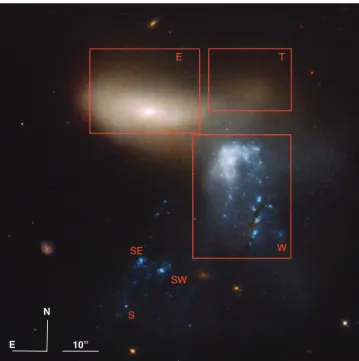
of a large elliptical and a blue irregular galaxy”. Figure1
dis-sects the system according the regions labeled byJohansson
(1988) andStiavelli et al. (1998). We will adopt their
defi-nition along this paper adding the prefix NGC 454.
The East part of the system, (labeled E in Figure 1,
NGC 454 E hereafter), identifies the early-type member of the pair. NGC 454 E is crossed by dust lanes and it is dis-torted by the interaction. The U, B, V Johnson and Gunn I
photometry byJohansson(1988) presented the East
mem-ber as a red elliptical with a luminosity profile that follows
closely an r1/4 law (de Vaucouleurs 1948) out to 1500
from
the galaxy center. TheStiavelli et al.(1998) high resolution
HST imaging, in the F450W, F606W, and F814W filters, shows that NGC 454 E is likely an S0. Their luminosity
pro-file, extending out to ' 3000, is much better fitted by two
components: an r1/4law describing the bulge plus an
expo-nential law (Freeman 1970) for a disk. The (B-V) color
pro-file indicates that the central part of the galaxy, i.e. r≤100, is
red with 1. (B-V) .1.4 while the outside region is slightly bluer with 0.8. (B-V) .1. The nucleus of NGC 454 E,
ob-served spectroscopically byJohansson(1988), revealed
sev-eral emission lines and matched two of the empirical
crite-ria proposed byShuder & Osterbrock (1981) for a Seyfert
galaxy: the line-width of Hα is larger than 300 km s−1and
the [OIII]λ5007˚A/Hβ ratio is larger than 3. However, none
of the high-excitation lines expected in this case, as HeII,
were detected (see alsoDonzelli & Pastoriza 2000;Tanvuia
et al. 2003). The AGN type of the nucleus has been
re-cently detailed byMarchese et al.(2012). Their analysis of
SWIFT, XMM-Netwon and Suzaku observations character-izes the NGC454 E nucleus as a “changing look” AGN. This is a class of AGN showing significant variation of the ab-sorbing column density along the line of sight.
The West region of the pair labeled in Figure1as W
(NGC 454 W hereafter) has been considered byJohansson
(1988) as the debris of an irregular galaxy. However, the
galaxy is so widely distorted by the on-going interaction
that the classification is difficult.Stiavelli et al.(1998)
sug-gested that it is the debris of a disk galaxy. NGC 454 W is
a starburst galaxy, as shown by the Hα image ofJohansson
(1988, their Figure 6a and 6b). The spectrum of NGC 454 W
shows emission lines whose ratios, according to the above authors, are due to photo-ionization by star formation and shock heating.
The NGC 454 E region is particularly distorted in the North-West side. This region, label as T (NGC 454 T
here-after) in Figure1, has been studied byStiavelli et al.(1998)
which found this is composed by a mix of the stellar popu-lations of the NGC 454 E and the NGC 454 W. Moreover, they found a similarity between the color of NGC 454 T re-gion and that of the nearby sky and speculated about the presence of a faint tail of stripped material in this region not detected by the HST observations.
The picture of the NGC 454 system is completed by three blue knots, NGC 454 SW, NGC 454 SE and NGC 454 S, well detached from NGC 454 E, and likely
con-nected to NGC 454 W (Johansson 1988;Stiavelli et al. 1998).
Johansson (1988) suggested that these are newly formed
globular clusters of 3×10⁶ M
and 1-5×10⁷ years stellar
age. Recently several investigations suggest that young in-dependent stellar systems at z ' 0 start to form in tidal
debris (see e.g. review byLelli et al. 2015).
Table 1 summarizes some basic characteristics of
NGC 454 E and W which appear as a prototype of an
en-counter/merger (∆Vhel=1±2 km s−1Tanvuia et al.(2003))
between a late and an early-type galaxy, this latter having an active and peculiar Seyfert-like nucleus. Therefore, the study of this system can make progresses in our understanding of the effects of a wet interaction.
ob-Table 1. NGC 454 system basic properties from the literature
NGC 454 E Ref.
Morphology E/S0 pec (1,2)
R.A. (2000) 1h14m25.2s (3) Decl. (2000) -55◦23’ 47” (3) Vhel 3635±2 km s−1 (3) (B − V )0 0.80 (1) (U − B)0 0.31 (1) LX (0.1-0.3 keV) XMM 2.8 1039erg cm−2s−1 (4)
LX (0.1-0.3 keV) Suzaku 5.6 1039erg cm−2s−1 (4)
LX (0.1-0.3 keV) XMM 2.5 1042erg cm−2s−1 (5)
LX (0.1-0.3 keV) Suzaku 7.2 1042erg cm−2s−1 (5)
LX (14-150 keV) XMM 4.8 1042erg cm−2s−1 (5)
LX (14-150 keV) Suzaku 1.4 1042erg cm−2s−1 (5)
NGC 454 W
Morphology Irr, (disrupted) Sp (1,2)
R.A. (2000) 1h14m20.1s (3) Decl. (2000) -55◦24’ 02” (3) Vhel 3626±2 km s−1 (3) (B − V ) 0.32 (1) (U − B)0 -0.22 (1) M(H2) [108M ] < 2 (6) Vhel adopted [km s−1 3645 (7) Distance [Mpc] 48.5±3.4 (7) scale [kpc arcsec−1] 0.235 (7)
References: (1)Johansson(1988) provides the mean corrected radial velocity; the morphology is uncertain (2)Stiavelli et al.
(1998); (3) the Heliocentric velocities of the E and W components are derived fromTanvuia et al.(2003) and are consistent with the systemic velocity Vhel=3645 provided by
NED we adopted; (4) Braito Valentina private communication; (5)Marchese et al.(2012) (6)Horellou & Booth(1997); (7) The
adopted heliocentric velocity and the distance (Galactocentric GSR) of the NGC 454 system are from NED.
servational information: (1) the investigation of the multi-wavelength structure of NGC 454 E via the optical and UV surface photometry and (2) the analysis of the kinematics of the ionized gas component. The Galaxy Evolution Explorer (Morrissay et al. 2007, GALEX) showed the strength of UV observations in revealing rejuvenation episodes in otherwise
old stellar systems (see e.g.Rampazzo et al. 2007;Marino et
al. 2011;Rampazzo et al. 2011, and references therein). In this context, we investigate the Near UV (NUV hereafter) stellar structure of the NGC 454 system using Swift UVOT
UV images (see also Rampazzo et al. 2017, and references
therein). In order to study the ionized gas, connected to the ongoing star formation, we use the SOAR Adaptive Module (SAM) coupled with a Fabry-Perot to investigate its distri-bution, the 2D velocity and velocity dispersion fields of the Hα emission in NGC 454 W and in NGC 454 SW and SE stellar complexes, likely debris of NGC 454 W. We finally attempt to derive the parameters and the merger history of the system using simulations.
The paper is organized as follows. In Section 2 we
present SWIFT-UVOT (§ 2.1) and the SAM+Fabry-Perot
(§ 2.2) observations of NGC 454 and the reduction
tech-niques used. The Swift-UVOT surface brightness photometry
is presented in §3. The ionized gas kinematics is presented in
N
E 10”
Figure 1. Color composite image of the NGC 454 system ob-tained with HST-Wide Field Planetary Camera 2 in the F450W (B), F606W (V), and F814W (I) filter byStiavelli et al. (1998). The figure highlights the different regions of the system follow-ingJohansson(1988) E and W areas include the early-type and the late-type member of the pair, respectively; S, SW and SE are knots likely connected to the W member. T is an area introduced byStiavelli et al.(1998) (see text). The size of the FOV is 1.660.
§4, the diagnostic digrams of H ii complexes are discussed in
§5, while §6considers the Hα line profile decomposition. In
§7our results are discussed in the context of galaxy-galaxy
interaction and compared with Smoothed Particle Hydro-dynamic (SPH) simulation with chemo-photometric
imple-mentation in §7.2. Finally in §8, we give the summary and
draw general conclusion.
2 OBSERVATION AND DATA REDUCTION
2.1 SWIFT-UVOT observations
UVOT is a 30 cm telescope in the SWIFT platform
operat-ing both in imagoperat-ing and spectroscopy modes (Roming et al.
2005). We mined the UVOT archive in the ASDC-ASI Science
Data Center retrieving the 00035244003 product including images of the NGC 454 system in all six filters available.
Ta-ble3gives the characteristics of these filters and calibrations
are discussed inBreeveld et al.(2010,2011).
The archival UVOT un-binned images have a scale of
0.005/pixel. Images were processed using the procedure
de-scribed in http://www.swift.ac.uk/analysis/uvot/. All the images taken in the same filter are combined in a single image using UVOTSUM to improve the S/N and to enhance the visibility of NUV features of low surface brightness. The fi-nal data set of the U V W 2, U V M 2, U V W 1, U , B, V images
have total exposure times reported in Table3.
UVOT is a photon counting instrument and, as such, is subject to coincidence loss when the throughput is high,
whether due to background or source counts, which may result in an undercounting of the flux affecting the brightness
of the source. Count rates less than 0.01 counts s−1pixel−1
are affected by at most 1% and count rate less than 0.1
counts s−1pixel−1 by at most 12% due to coincidence loss
(Breeveld et al. 2011, their Figure 6).
Coincidence loss effects can be corrected in the case
of point sources (Poole et al. 2008; Breeveld et al. 2010).
For extended sources a correction process has been per-formed for NGC 4449, a Magellanic-type irregular galaxy
with bright star forming regions, byKarczewski et al.(2013).
Even though their whole field is affected, the authors calcu-late that the statistical and systematic uncertainties in their total fluxes amount to ≈ 7-9% overall, for the NUV and the optical bands.
We checked, indeed, that in UV filters the coincidence losses may involve only few central pixels of the Irr galaxy,
i.e., NGC 454 W, never exceeding 0.1 count s−1px−1(in
par-ticular, the maximum value of the count rates is 0.043, 0.028,
and 0.047 count s−1px−1in U V W 2, U V M 2 and U V W 1
fil-ters respectively). Our NUV images are very slightly affected so we decided do not account for this effect. Optical images are more affected. In the NGC 454 W region the effect
re-mains ≤ 0.1 count s−1 px−1 in all the bands, in particular
it reaches 0.09, , 0.08, and 0.096 count s−1px−1in the U , B
and V filters respectively. As far as NGC 454 E is concerned,
in the U filter count rates are at most 0.084 count s−1px−1,
and reach 0.2 in the B and V bands in the inner 500. So, we
add to the photometric error in Table 3 a further error of 12% in optical bands to account for this effect.
We compared our total magnitudes in Table 3 with
Prugniel & H´eraudeau(1998) which reported a total mag-nitude B=13.32±0.05 and 13.44±0.064, respectively for the whole NGC 454 system and for NGC 454 W. Once our mea-sures are scaled to the Vega system (B=B[AB]+0.139) we have B=13.43±0.15 and B=13.65±0.12, in very good agree-ment with previous estimates.
Our (B − V ) color, integrated within a 3100 aperture
and corrected for galactic absorption for NGC 454 E and NGC 454 W is 0.88±0.11 and 0.48±0.06, respectively, to be
compared with 0.80 and 0.32 fromJohansson(1988).
2.2 Fabry-Perot observation
Fabry-Perot (FP hereafter) observations1have been carried
out on Sept 30th 2016 as part of the SAM-FP Early Sci-ence run at SOAR 4.1m telescope at Cerro Pachon (Chile). SAM-FP is a new instrument, available at SOAR, combining
the adaptative optics SAM (Tokovinin et al. 2010a,b) and a
scanning Queensgate ET70 Etalon (Mendes de Oliveira et
al. 2017). The SAM module has been conceived to deliver
a 0.0035 angular resolution across a 30×30FoV, depending on
atmospheric condition, using Ground Layer Adaptive Op-tics (GLAO). The SAM instrument detector is a 4K×4K
CCD with a scale image scale of 0.000454 (physical pixel of
15µ) on the sky (Fraga et al. 2013). The present
observa-tions have been binned over 4×4 pixels resulting in a scale
of 0.0018/px. The interferometer used is a ET70 Queensgate
1 All Fabry-Perot data (cubes and moment maps) are available
at cesam.lam.fr/fabryperot/
scanning FP with an order of p=609@Hα. The FP piezos are driven by a CS100 controller, positioned at the telescope.
Ta-ble2gives the journal of observation with the characteristic
of the etalon we used. At the center of the Free Spectral
Range we adopt the systemic velocity of 3645 km s−1
pro-vided by NED (see alsoDonzelli & Pastoriza 2000; Tanvuia
et al. 2003, as more recent and independent sources). Data have been reduced using home made Python macros to handle Multi Extension Files from SAM and
building the data cube, some IRAF2 specific tasks and
Ad-hocw 3 software procedures have been used to handle the
cube. The data reduction procedure has been extensively
described byAmram et al.(1996) andEpinat et al.(2008).
The first step, before the phase correction, is to perform the standard CCD data reduction by applying bias and flat-field corrections under IRAF as well as the cosmic removal using
L.A.cosmic procedure (van Dokkum 2001). Linear
combi-nations of dark images have been used to removed CCD patterns in different frames.
In addition to these canonical operations, it is necessary to check and correct for several effects, such as, misalignment of data cube frames (due to bad guiding), sky transparency variation throughout the cube, and seeing variation. Mis-alignment variation across the 43 frames of the data cube is less than half pixel, thus it is negligible. The sky trans-parency has been corrected using a star in the FoV. It varies between 81% to 98% during the observation: each frame has been corrected accordingly using one channel as a reference. The same star is also used to map the corrected seeing
varia-tion ranging from 0.0071 to 0.0090. We then applied a 2D spatial
Gaussian smoothing equivalent to the worse estimated
cor-rected seeing (0.0090). Phase map and phase correction have
been performed using the Adhocw package and by scanning
of the narrow Ne 6599˚A line under the same observing
con-ditions. The velocities measured are very accurate compared
to the systemic velocity in Table1, with an error of a
frac-tion of a channel width (i.e., < 3 km s−1) over the whole
FoV. The signal measured along the scanning sequence was separated into two parts: (i) an almost constant level
pro-duced by the continuum light in a 15˚A passband around Hα
(continuum map, not presented in this work); (ii) a varying part produced by the Hα line (Hα integrated flux map). The continuum is computed by taking the mean signal outside the emission line. The Hα integrated flux map was obtained by integrating the monochromatic profile in each pixel. The
velocity sampling was 11.6 km s−1. Strong OH night-sky
lines passing through the filters were subtracted by
deter-mining the level of emission away from our target (Laval et
al. 1987).
The velocity dispersion (σ hereafter) is derived from the determination of the FWHM from the determined profile. Then the real dispersion velocity is found supposing that different contributions follow a gaussian function.
σ2real= σ 2 obs− σ 2 th− σ 2 inst
2 IRAF is distributed by the National Optical Astronomy
Obser-vatories, which are operated by the Association of Universities for Research in Astronomy, Inc., under cooperative agreement with the National Science Foundation.
Table 2. Instrumental setup
Fabry-Perot Parameters Values
Telescope SOAR 4.1m
Date Sept. 30th2016
Instrument SAM-FPa
Detector CCD
Pixel size (binned) 0.0018/px (0.000454×4)
Calibration neon light (λ) 6598.95 ˚A
Resolution (λ/∆λ) 10700
Filter Characteristics
Filter Central wavelength 6642˚A
Filter Transmission 80%@6642˚A
Filter FWHM (∆λ) 15˚A
Interferometer Characteristics
Interferometer order at Hα 609
Free spectral range at Hα (km s−1) 498
Number of scanning steps 43
Sampling steps 0.26 ˚A (11.60 km s−1)
Total Exposure Time 1.1h (90s/channel)
aTokovinin et al.(2010a,b)
where σinst = 12.82 km s−1 is the instrument
broad-ening deduced from the Ne calibration lamp and σth= 9.1
km s−1is the thermal broadening of the Hα line.
3 SURFACE PHOTOMETRY FROM
SWIFT-UVOT OBSERVATIONS
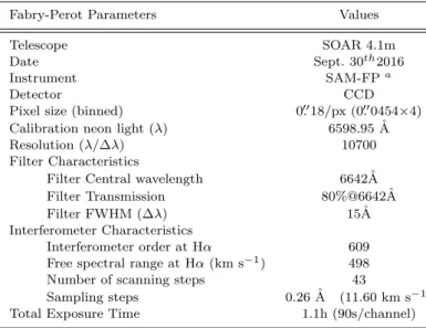
The color composite images in optical and NUV bands from the Swift-UVOT observations are shown in the top panels of
Figure2. Images show that the NGC 454 W emission
dom-inates in the NUV bands. In NUV NGC 454 W1- W6 com-plexes appear included in a unique envelope which elongates up to NGC 454 SW and SE. In NUV two complexes, already
revealed in Hα byJohansson(1988), are projected between
NGC 454 SE and NGC 454 W. NGC 454 S, shown in
Fig-ure1, appears connected to NGC 454 SW.
We derived the luminosity profiles and (U V M 2 − V ) and (B − V ) color profiles of NGC 454 E. They are shown
in the middle and bottom panels of Figure 2. Luminosity
profiles have been derived using the task ELLIPSE in the
package IRAF (Jedrzejewski 1987). These are not corrected
for galactic extinction. Since we aim at parameterizing the
galaxy structure we have truncated the profile at ≈3500(a1/4
= 2.43) where the distortion by NGC 454 W, in particular in NUV, becomes dominant.
The (B −V ) color profile tends to become bluer with the
galacto-centric distance as shown in Stiavelli et al. (1998).
The trend is much clear along the (U V M 2−V ) color profile.
Stiavelli et al.(1998) parametrized the HST luminosty profiles with a composite bulge plus disk model. Due to our poorer resolution and PSF, to parametrize the trend of
op-tical and NUV surface brightness profiles we adopt a S´ersic
r1/n law (Sersic 1968), widely used for early-type galaxies
as a generalization of the r1/4 de Vaucouleurs (1948) law
(see e.g.Rampazzo et al. 2017, and references therein). We
best fit a S´ersic law convolved with a PSF, using a custom
IDL routine based on the MPFit package (Markwardt et al.
2009), accounting for errors in the surface photometry. The
PSF model is a Gaussian of given FWHM and the convo-lution is computed using FFT on oversampled vectors. We use the nominal value of the FWHM of the PSF of the UVOT
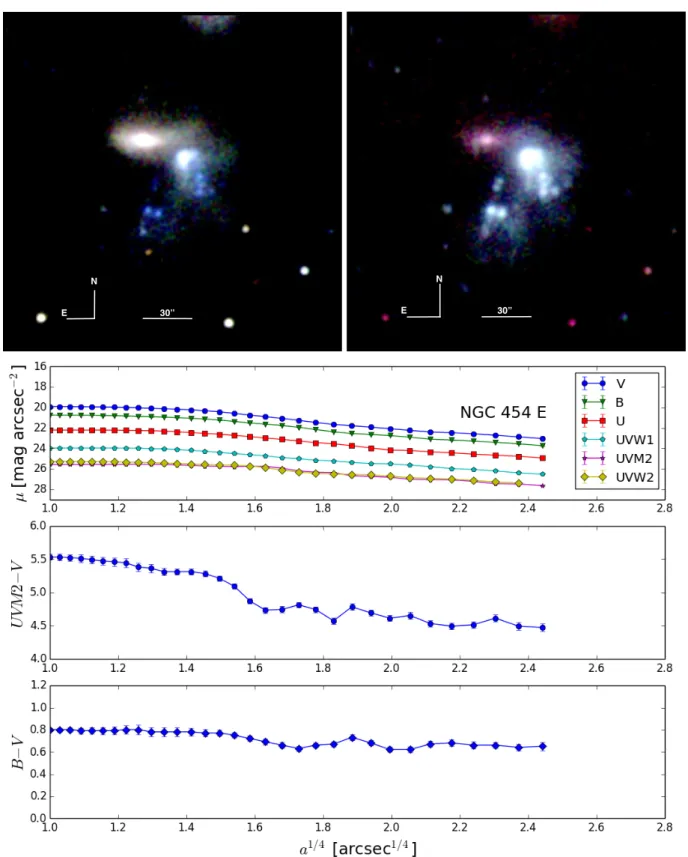
filters. The residuals, µ − µSersic, are shown in two panels
of Figures3, together with the values of the S´ersic indices
for each of the UVOT bands reported in the top right
cor-ner of the two panels. The S´ersic indices are in the range
1.09±0.13≤ n ≤1.79±0.06
We remind that the S´ersic law has three special cases
when n=1, the value for an exponential profile, and n = 0.5, for a Gaussian luminosity profile and n=4 for a bulge. The
range of our S´ersic indices suggests that NGC 454 E has a
disk. Residuals in Figure3shows a trend starting at about
a1/4' 1.600
consistently with a clear change in color in the (U V M 2 − V ) color profile.
4 IONIZED GAS MOMENT MAPS
We extract from SAM+FP observations the monochromatic Hα emission map, the radial velocity and velocity dispersion
maps. In Figure4we show HST F450W image (Stiavelli et
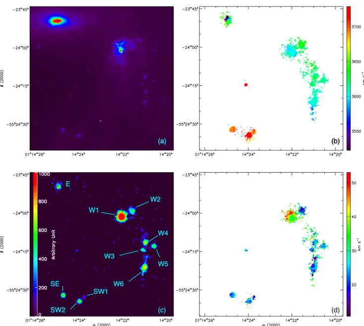
al. 1998) (top left panel) on the same scale with our Hα monochromatic map (bottom left panel), heliocentric radial velocity map (top right panel), and velocity dispersion map (bottom right panel) of the system, corrected from broaden-ing.
4.1 Hα monochromatic intensity map
Both narrow band imaging (Johansson 1988) and
spec-troscopy (Donzelli & Pastoriza 2000; Tanvuia et al. 2003)
revealed Hα emission in the NGC 454 system. The bottom
left panel of Figure4 shows the Hα monochromatic
inten-sity (I) map detected by our FP observations. Hα emis-sion is revealed in the nucleus of NGC 454 E, in the NGC 454 W region and in the NGC 454 SE and SW complexes. NGC 454 W region shows a structured Hα emission. In this region we spot 6 complexes we labeled from W1 to W6,
roughly from North to South, as shown in Figure4(bottom
left panel).
NGC454 E has a Seyfert 2-type nucleus with broad, 250
and 300 km s−1, emission line profiles (Johansson 1988).
That fits into the Free Spectral Range of our etalon (almost
500 km s−1). We apply a 5×5 px (0.212×0.212 kpc) boxcar
smoothing to enhance the signal in the nuclear zone. The
emission extends 3.003 × 2.000 (0.8 kpc × 0.7 kpc) around the
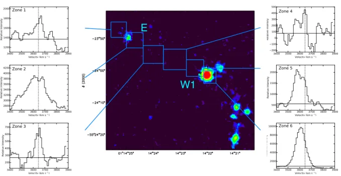
center of NGC 454 E. Integrating the signal within boxes
(see Figure 5) along the line connecting the NGC 454 E
nucleus to the brightest complex of NGC 454 W (we labeled W1) we reveal emission lines whose profiles have complex shapes.
The W1 complex is the brightest in NGC 454 W,
show-ing a nearly circular shape and a diameter of 5.007 (1.3 kpc);
the W6 complex is the larger, extending to 8.005 (2 kpc).
In the NUV map we may distinguish all the W1–W6 com-plexes but they appear more extended and interconnected than shown by our FP observations.
The NGC 454 SW and NGC 454 SE emission complexes
shown in Figure4 are relatively weaker than the W1–W6
complexes. We need to integrate the signal within 5×5 pix-els bins to detect a connection between these complexes as
30” N
E 30”
N
E
Figure 2. (top panels) Optical image (U blue, B green, V red), on the left and UV color composite image (U V W 2 blue, U V M 2 green, U V W 1 red), on the right, of the NGC 454 system as observed by Swift-UVOT. The images have been smoothed 2 × 2 pixels (resulting 100×100resolution). The total Field of View is 40×40. (middle panel) Luminosity profiles of NGC 454 E in the optical and NUV bands.
Profiles are not corrected for coincidence loss and galactic absorption. (bottom panels) (M 2 − V ) and (B − V ) color profiles in [AB] magnitudes corrected for galactic absorption.
Table 3. Swift-UVOT integrated magnitudes
Filter U V W 2 U V M 2 U V W 1 U B V
Central λ 2030[˚A] 2231[˚A] 2634[˚A] 3501[˚A] 4329[˚A] 5402 [˚A]
PSF (FWHM) 200.92 200.45 200.37 200.37 200.19 200.18
Zero Pointa 19.11±0.03 18.54±0.03 18.95±0.03 19.36±0.02 18.98±0.02 17.88±0.01
Total exp. time 1325 [s] 2255 [s] 3040 [s] 652 [s] 453 [s] 762[s]
Integrated magnitudes [AB mag] [AB mag] [AB mag] [AB mag] [AB mag] [AB mag]
NGC 454 E 17.96±0.13 17.83±0.25 16.61±0.28 15.15±0.14 13.77±0.18 13.20±0.18
NGC 454 W 15.32±0.15 15.16±0.13 14.90±0.09 14.46±0.12 13.51±0.20 13.13±0.28
aprovided byBreeveld et al.(2011) for converting UVOT count rates to AB mag. (Oke 1974).
Figure 3. Residual from the fit of a single S´ersic r1/nlaw of the
optical (top panel) and NUV (bottom panel) luminosity profiles. The value of the S´ersic indices, for each UVOT band are reported on the top right side of the figure. The values of the indices suggest the presence of a disk structure.
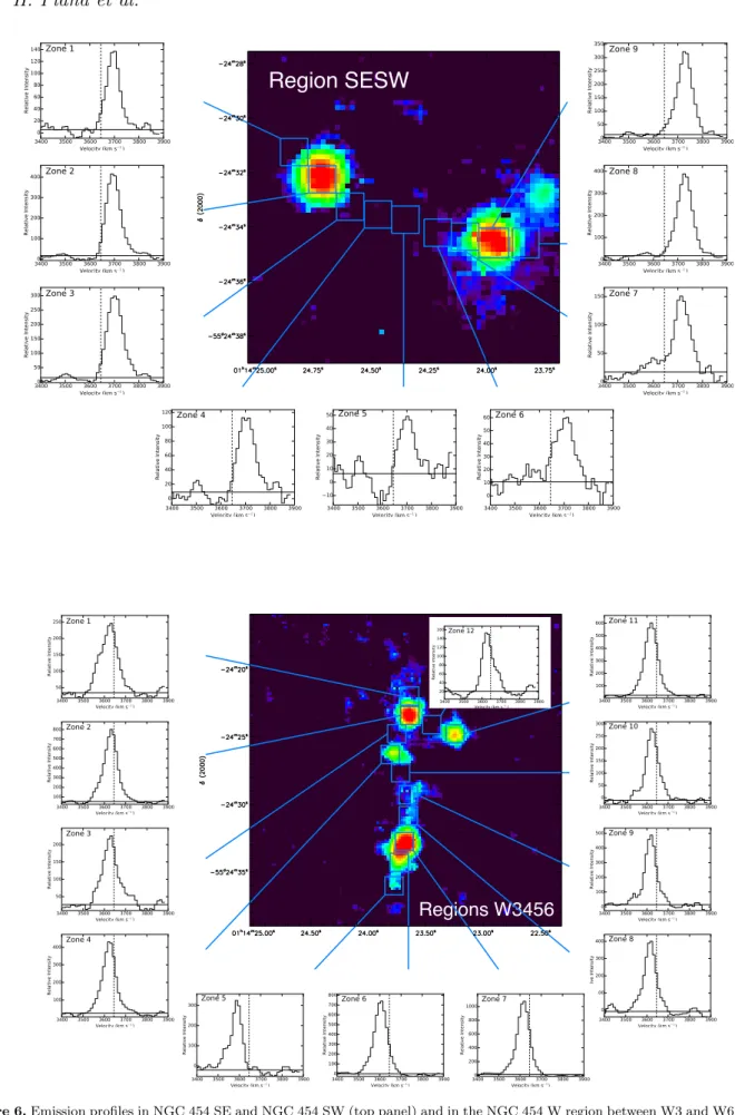
shown in the Johansson’s Hα narrow band image. The
bot-tom panels of Figure6show emission lines profiles in several
areas of NGC 454 W, NGC 454 SE and NGC 454 SW.
Both the Hα image by Johansson (1988) and in our
NUV images show an elongated emission region between NGC 454 SW and NGC 454 W1 complex, weaker than the other regions. We also detect emission in between the SW,
SE complex and the SW1 region (see Figure4). Our
observa-tion is showing a much smaller extension (1.001 corresponding
to 0.3 kpc) compared toJohansson(1988).
To summarize, the W1–W6 as well as SW and SE in NGC 454 W are huge (up to 2 kpc wide) complexes of ion-ized interstellar medium (ISM hereafter). Ionion-ized ISM is also found in NGC 454 E center and along the line connecting it to NGC 454 W1 complex.
4.2 Radial velocity map
Figure4(top right panel) shows the 2D radial velocity, Vr,
map of NGC 454. NGC 454 E velocity field is difficult to interpret because this object is an AGN showing large line profiles, almost covering our free spectral range.
Neverthe-less, a velocity gradient of 130 km s−1, across 400(0.94 kpc),
is measured.
Velocities in the NGC 454 W range over 70 km s−1, from
maximum of 3645 km s−1measured in the W2 complex to a
minimum of 3575 km s−1in the southern tip of W6 complex.
None of the W1–W6 complexes has a rotation pattern. The
W6 complex shows a velocity gradient of 35 km s−1across a
length of 8.003 (1.95 kpc). The NGC 454 SW and NGC 454 SE
complexes do not present velocity gradients. With respect to the W1-W6 complexes the SW and SE complexes are
receding with a systemic velocity of 3725 km s−1 and 3691
km s−1, respectively, with a velocity difference ∆V
'115-145 km s−1with respect to W1 complex.
4.3 Velocity dispersion map
The velocity dispersion, σ, map is shown in the bottom right
panel of Figure4. As mentioned before, NGC 454 E shows
very broad profiles, very close to our free spectral range. In those conditions, we prefer not to show a velocity dispersion map for this galaxy. We measure σ values ranging from 14 to
42 km s−1 in the W3, W4, W5, W6 complexes. σ values of
NGC 454 SW and NGC 454 SE are homogeneous, between
20 and 29 km s−1 . We point out that values exceeding 10
- 20 km s−1 indicate supersonic motions (see e.g.Smith &
Weedman 1970). The W1 complex shows the highest values,
up to 66 km s−1, while in the W2 complex, σ ranges from
13 to 32 km s−1.
4.4 Emission between HII regions
Figure 5 and Figures 6 show several regions in
be-tween NGC 454 E and NGC 454 W1 (Figure 5),
NGC 454 SW and NGC 454 SE (Figure6top) and between
NGC 454 W3 W4 W5 and W6 (Figure6bottom).
Figure5, regions 1 and 2 show the emission centered in
the elliptical. As mentioned before, the center of NGC 454 E has a broad emission as shown in region 2. With an emission peak above 3800 (in relative units) and a background of 2500, region 2 has a very high intensity considering that
W1 W2 W4 W5 W3 W6 SE SW1 SW2 E (a) (b) (c) (d) W1 W2 W4 W5 W3 W6 SE SW1 SW2 E (a) (b) (c) (d) W1 W2 W4 W5 W3 W6 SE SW1 SW2 E (a) (b) (c) (d) W1 W2 W4 W5 W3 W6 SE SW1 SW2 E (a) (b) (c) (d)
Figure 4. (a) HST F450W image of the NGC 454 system (Stiavelli et al. 1998), (b) 2D velocity field of Hα emission, centred on the NGC 454 systemic velocity, (c) monochromatic Hα map, and (d) Hα velocity dispersion map, corrected from broadening.
background is dominated by poisson noise and even if
we consider that the profile has a FWHM of 300km s−1
(compared to the 500 km s−1of the free spectral range), we
still see the emission of the center of the elliptical. Regions 3 and 4 show areas in between NGC 454 E and NGC 454 W1, when region 3 shows a confortable emission line, region 4 shows the limit of our detection with an emission peak at one σ above the continuum level. Regions 5 and 6 show NGC 454 W1 emission, a detailed discussion about this
latest is given in subsection 5.2and section6.
Figure 6 (top) shows emission profiles between
the SE and SW regions. Emission is very clear across both regions. No substantial velocity gradient is visible
even if the radial velocity of SW is 30 km s−1lower than SE.
Figure 6 (bottom) shows the connection between the
remaining regions (NGC 454 W3 to W6). Emission is strong and it is clear that all regions are connected. Zones 1 and 12 show asymmetric profiles, probably due to a second compo-nent. A radial velocity gradient is visible between the south-ern tip with zone 5 and region 1.
5 HIIREGIONS DIAGNOSTIC DIAGRAMS
5.1 Description of the complexes
Complexes in NGC 454 W, share similar dynamical char-acteristics both with Giant H ii Regions and the so-called H ii Galaxies. Firstly, like GH iiRs, W1 has high supersonic
profiles (Smith & Weedman 1970) and, secondly, the
high velocity dispersion surrenders high monochromatic emission. Several studies using Fabry-Perot interferometer (Mu˜noz-Tu˜n´on et al. 1996) found this signature in nearby
E
W1
Figure 5. Emission profiles in the region NGC 454 E and NGC 454 W1. The vertical dotted line indicates the systemic velocity adopted Vhel=3645 km s−1.The horizontal line indicates the mean continuum level. The map corresponds to the monochromatic emission.
Giant H ii Region, like NGC 604. More recently, still using
Fabry-Perot and IFU spectroscopy Bordalo et al. (2009);
Moiseev & Lozinskaya (2012); Plana & Carvalho (2017), evidences have been found of such signature within dwarf H ii galaxies.
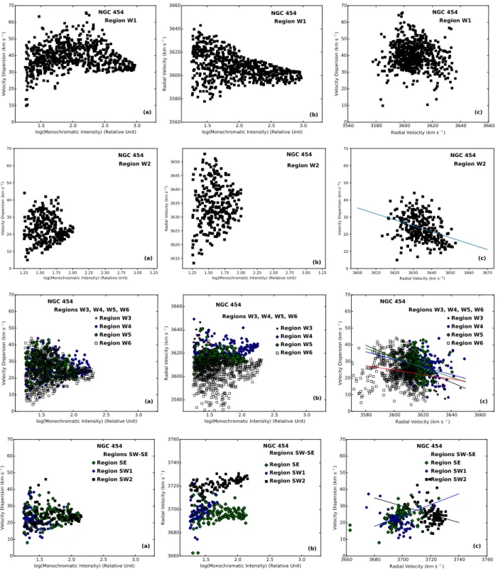
Figure 7 considers three different diagnostic diagrams
used to study the kinematics of H ii regions These diagnostic diagrams are shown for NGC 454 W complexes (W1-W6
identified in Figure4) and for NGC 454 SW and SE regions.
The W1 complex has the larger intensity range. We
will discuss the (I − σ) regimes in this region in Section5.2
with a statistical approach.
The panels (a) in Figure 7 represent the intensity vs
the dispersion velocity (sigma). The W2 – W6 as well as SW1, SW2 and SE complexes show similar intensity and sigma ranges. In W3 – W6 as well as NGC 454 SW and SE complexes the scatter of σ increases as the intensity
de-creases. As discussed byMoiseev & Lozinskaya(2012) (their
Figure 6) this shape is produced within star forming com-plexes with significant excursion of gas densities, indicating low density, turbulent ISM. At high density (high intensity) regime H ii regions have either nearly constant or low scat-ter σ. However, towards lower density (low intensity) the high perturbed/turbulent gas surrounding H ii regions may emerge so decreasing the intensity the σ scatter may in-crease. We have separated the different regions: W3, W4, W5 and W6 as SE, SW1 and SW2 complexes in these
dia-grams. The last row of Figure7shows the SE, SW1 and SW2
complexes I vs σ diagram, but none of the three complexes
shows a different pattern. Introduced byMu˜noz-Tu˜n´on et al.
(1996), the (I −σ) diagram has been used by those authors to
identify expanding shells by localising inclined bands. This interpretation is based on the fact that the velocity disper-sion should be higher at the center of the shell and the in-tensity lower because less material is crossed along the line of sight than at the shell inner and outer edges. Assuming
this pattern, the inclination of the band can also be inter-preted in term of age of the shell itself. As the shell ages, the velocity dispersion at the center decreases as well as the intensity difference between the center and inner edge
of the shell (see figure 3 inMu˜noz-Tu˜n´on et al. 1996). The
Moiseev & Lozinskaya(2012) interpretation tends to act for larger scales, where high velocity dispersion is not related to specific expanding shells, but rather belong to the diffuse low brightness emission.
The panels (b) in Figure 7represent the intensity vs.
radial velocity, (I − Vr), diagram of W1-W6 complexes in
NGC 454 W, and in the SW1, SW2 and SE.
The range of radial velocity, Vr, within complexes is
small, of the order of 20-40 km s−1 in the W3 – W6 and
NGC 454 SW1, SW2 and SE complexes. Large radial ve-locity excursion at all intensities is found in W2. The W3, W4, W5 and W6 complexes show different radial velocities, with W4 having the highest and W6 the lowest. W6 velocity range is larger because of the velocity gradient we already
mentioned in Section4. The separation in radial velocity
be-tween the SE, SW1 and SW2 complexes is shown in the plot
(b) of the last row of Figure7. The complex NGC 454 SE,
SW and SW2 have a small variation, 10-20 km s−1, of Vr
while the monochromatic intensity range is similar to W3 – W6 complexes. It also appears that SW1 complex has a closer radial velocity with SE than with SW2. According to (Bordalo et al. 2009) (their figure 13b), a vertical band in this diagram, representing a velocity variation in a short in-tensity range, means a radial motion such as an expansion, but it could also means an inflow. The physical mechanisms in action are several including turbulence, winds, flows, bub-bles or the self gravity of the complexes at different scales. Even if a vertical band can appear in the plot representing W2 (second row), it is difficult to interpret it as a signature of a radial motion, the intensity range being too wide.
Region SESW
Regions W3456
Figure 6. Emission profiles in NGC 454 SE and NGC 454 SW (top panel) and in the NGC 454 W region between W3 and W6 complexes (bottom panel). The vertical dotted line indicates the systemic velocity adopted Vhel=3645 km s−1.The horizontal line indicates the
1.5 2.0 2.5 3.0 log(Monochromatic Intensity) (Relative Unit) 0 10 20 30 40 50 60 70 Ve loc ity D isp er sio n (k m s − 1) NGC 454 Region W1 (a) 1.5 2.0 2.5 3.0 log(Monochromatic Intensity) (Relative Unit) 3560 3580 3600 3620 3640 3660 Ra dia l V elo cit y ( km s − 1) NGC 454 Region W1 (b) 3560 3580 3600 3620 3640 3660 Radial Velocity (km s−1) 0 10 20 30 40 50 60 70 Ve loc ity D isp er sio n (k m s − 1) NGC 454 Region W1 (c) 1.25 1.50 1.75 2.00 2.25 2.50 2.75 3.00 3.25 log(Monochromatic Intensity) (Relative Unit) 0 10 20 30 40 50 60 70 Ve loc ity D isp er sio n (k m s 1) NGC 454 Region W2 (a) 1.25 1.50 1.75 2.00 2.25 2.50 2.75 3.00 3.25 log(Monochromatic Intensity) (Relative Unit) 3615 3620 3625 3630 3635 3640 3645 3650 Ra dia l V elo cit y ( km s 1) NGC 454 Region W2 (b) 3600 3610 3620 3630 3640 3650 3660 3670 Radial Velocity (km s1) 0 10 20 30 40 50 60 70 Ve loc ity D isp er sio n (k m s 1) NGC 454 Region W2 (c) 1.5 2.0 2.5 3.0 log(Monochromatic Intensity) (Relative Unit) 0 10 20 30 40 50 60 70 Ve loc ity D isp er sio n (k m s − 1) NGC 454 Regions W3, W4, W5, W6 (a) Region W3 Region W4 Region W5 Region W6 1.5 2.0 2.5 3.0 log(Monochromatic Intensity) (Relative Unit) 3580 3600 3620 3640 3660 Ra dia l V elo cit y ( km s − 1) NGC 454 Regions W3, W4, W5, W6 (b) Region W3 Region W4 Region W5 Region W6 3580 3600 3620 3640 3660 Radial Velocity (km s−1) 0 10 20 30 40 50 60 70 Ve loc ity D isp er sio n (k m s − 1) NGC 454 Regions W3, W4, W5, W6 (c) Region W3 Region W4 Region W5 Region W6 1.5 2.0 2.5 3.0 log(Monochromatic Intensity) (Relative Unit) 0 10 20 30 40 50 60 70 Ve loc ity D isp er sio n (k m s − 1) NGC 454 Regions SW-SE Region SE Region SW1 Region SW2 (a) 1.5 2.0 2.5 3.0 log(Monochromatic Intensity) (Relative Unit) 3660 3680 3700 3720 3740 3760 Ra dia l V elo cit y ( km s − 1) NGC 454 Regions SW-SE Region SE Region SW1 Region SW2 (b) 3660 3680 3700 3720 3740 3760 Radial Velocity (km s−1) 0 10 20 30 40 50 60 70 Ve loc ity D isp er sio n (k m s − 1) NGC 454 Regions SW-SE Region SE Region SW1 Region SW2 (c)
Figure 7. From top to bottom: panels plot (a) (I − σ), panels (b) (I − Vr), panels (c) (Vhel− σ) diagnostic diagrams in W1-W6 complexes
in NGC 454 W and in the NGC 454 SE and SW complexes. The plot results from a single Gaussian fit to the line profile. Solid lines in Vr− σ diagrams represent the linear regressions applied when the Pearson’s correlation test is robust.
in the same regions.Bordalo et al.(2009) pointed out that a
dependence between the variables may indicate systematic relative motion of the clouds in the complex. They presented
an idealized pattern for this diagram. Inclined (Vr− σ)
pat-terns would represent systematic motion like Champagne flows, such that cloud of gas with high σ moves away from us (positive slope) or toward us (negative slope).
We perform a standard Pearson’s product-moment crelation test for the different complexes of NGC 454, in or-der to show the existence of systematic motions mentioned above. Except for W1 and SW1, all regions show weak-moderate correlation, according this test. W2 has a corre-lation coefficient of -0.34, W3 of -0.43, W4 of -0.23, W5 of -0.27, W6 of -0.17. The SE and SW2 regions also have a
Log(Intensity) (R.U.) V elocity Dispersion ( km .s − 1) 1.5 2 2.5 3 10 20 30 40 50 60 X (arcsec) Y (arcsec) 7 6 5 4 3 2 1 0 0 1 2 3 4 5 6 7
Figure 8. (bottom panel) The 3×3 pixels sampling of the NGC 454 W1 complex. (top panel) (I − σ) plot. The colors high-light two regions, the central and outskirts, with different regimes (see Section5.2for details). Top profile shows a typical monochro-matic emission representative of the blue points, and bottom pro-file representative of the red points.
weakmoderate correlation with a coefficient of 0.48 and -0.25. All of them with a 99.9% confidence level. The case of SW1 is a bit more complex. The Pearson test is not conclu-sive and we decide to use a robust correlation test in order to put lower weight in marginal points. Using the WRS2 package in R, we found a correlation of -0.2 with a 90% confidence level.
We perform a simple linear regression (the solid line
in Figure 7 panels (c)) for the regions where the Pearson
test shows a weak-moderate correlation: W2 to W6, SE and SW2. In this context W2 and SW2 regions can be inter-preted as complexes with relatively high dispersion, moving toward the observer (negative slope). In the case of the SE
complex, the slope is positive and it can be interpreted as a complex moving away from the observer.
Previous studies, on Giant H ii Region or emitting dwarf galaxies, also used those diagnostic diagrams when these ob-jects are smaller and the scale resolution much smaller than
here. For example NGC 604 study fromMu˜noz-Tu˜n´on et al.
(1996) or dwarf galaxies fromMoiseev & Lozinskaya(2012)
orBordalo et al.(2009) have respectively scale resolution of
3.31pc/00and 21pc/00. This is ten times smaller than our
ob-ject. Even though, we found remarkable similarities between diagnostics diagrams.
5.2 Statistical analysis of the (I − σ) diagrams for
W1 complex
We use the R statistical package (R Development Core Team 2009) to analyze the (I −σ) diagram of the W1 complex. R is largely use in different statistical analysis. The Mclust
rou-tine only has been recently used in astrophysics by (Einasto
et al. 2010) to detect structure in galaxies clusters. We aim at finding how many independent components are present (task Mclust), to locate them in the diagram and in the σ map (so-called geographic location). Mclust is a R func-tion for model-based clustering, classificafunc-tion, and density estimation based on finite Gaussian mixture modeling. An integrated approach to finite mixture models is provided, with routines that combine model-based hierarchical
clus-tering and several tools for model selection (see Fraley &
Raferty 2007).
For a bivariate random sample x be a realization from a finite mixture of m > 1 distributions, it should follow
p(x|π, {µk, Σk}) =
X k
πkφ(x|µk, Σk), (1)
where φ is the multivariate normal density
φ(x|µ, Σ) = (2π)−d/2|Σ|−1/2exp {−1
2(x − µ)
0
Σ−1(x − µ)},
(2)
π = {π1, ..., πm} are the mixing weights or probabilities
(such that πk> 0 andPmk πk = 1), (µk, Σk) are the mean
the covariance matrix of the component k, and d is the di-mension of the data. A central question in finite mixture modeling is how many components should be included in the mixture. In the multivariate setting, the volume, shape, and orientation of the covariances define different models (or parametrization) with their different geometric charac-teristics. In Mclust, the number of mixing components and the best covariance parameterization are selected using the
Bayesian Information Criterion (BIC). The task outputs µk,
Σk and πk for k running from 1 to m. Mclust also relates
each element in the dataset to a particular component in the mixture. To gain some flexibility on this classification, we combine the central result of Mclust, the number of com-ponents m, with the result of another R task: the mvnor-malmixEM function.
This task belongs to the mixtools package, which provides a set of functions for analyzing a variety of finite mixture models. The general methodology used in mixtools involves the representation of the mixture problem as a
3400 3500 3600 3700 3800 Ve loc ity (k m s − 1) 0 20 40 60 80 100
Zone
W1-3
3400 3500 3600 3700 3800 Ve loc ity (k m s − 1) 0 20 40 60 80 100 120Zone
W1-2
3400 3500 3600 3700 3800 Ve loc ity (k m s − 1) 0 20 40 60 80Zone
W1-1
3400 3500 3600 3700 3800 Ve loc ity (k m s − 1) 0 20 40 60 80 100 120Zone
W1-13
3400 3500 3600 3700 3800 Ve loc ity (k m s − 1) 0 20 40 60 80 100Zone
W2-1
3400 3500 3600 3700 3800 Ve loc ity (k m s − 1) 0 10 20 30 40 50 60 70Zone
W1-4
3400 3500 3600 3700 3800 Ve loc ity (k m s − 1) 0 50 100 150Zone
W1-12
3400 3500 3600 3700 3800 Ve loc ity (k m s − 1) 0 10 20 30 40 50 60 70 80Zone
W1-5
3400 3500 3600 3700 3800 Ve loc ity (k m s − 1) 0 50 100 150 200 250Zone
W1-11
3400 3500 3600 3700 3800 Ve loc ity (k m s − 1) 0 10 20 30 40 50 60 70Zone
W1-6
3400 3500 3600 3700 3800 Ve loc ity (k m s − 1) 0 200 400 600 800Zone
W1-7
3400 3500 3600 3700 3800 Ve loc ity (k m s − 1) 0 20 40 60 80Zone
W1-8
3400 3500 3600 3700 3800 Ve loc ity (k m s − 1) 0 20 40 60 80 100Zone
W1-9
3400 3500 3600 3700 3800 Ve loc ity (k m s − 1) 0 20 40 60 80 100 120Zone
W1-10
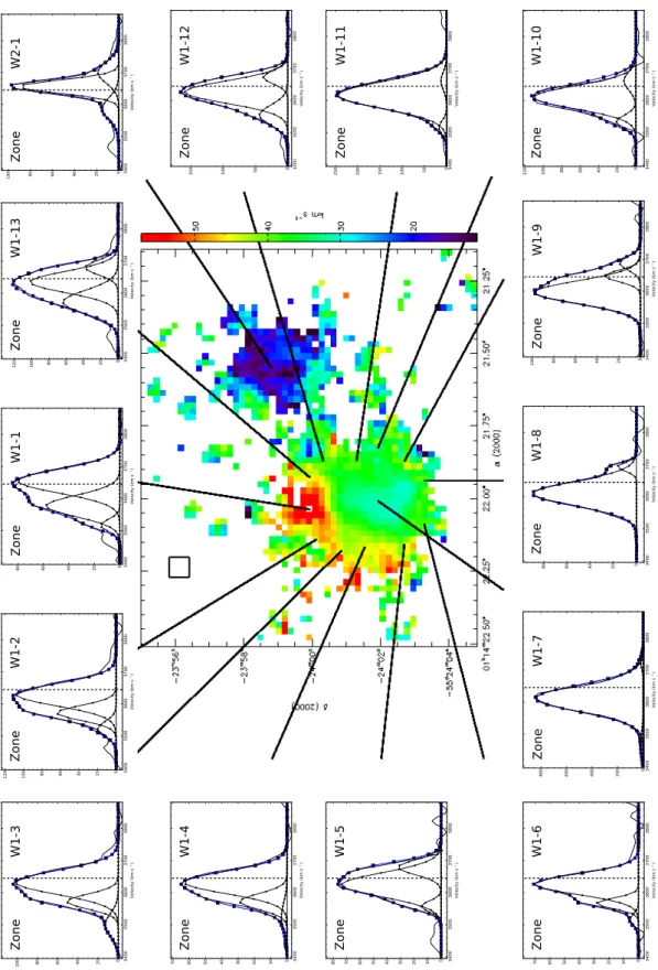
Figure 9. Integrated profiles in NGC 454 W1 and W2. Three Gaussian components fit of the emission lines in NGC 454 W1 and W2 complexes. Results of the fitting are reported in Table3. The vertical dotted line indicates the systemic velocity adopted Vhel=3645
km s−1.The horizontal line indicates the mean background level. The small square approximatively represents the size of the area of the integrated profiles (3 × 3px or 0.5400× 0.5400). The map corresponds to the dispersion velocity field, corrected from broadening.
Table 4. Hα line profiles Gaussian components in Region W1
Regions Component 1 Component 2 Component 3
I Vr σ I Vr σ I Vr σ
R.U. [km s−1] [km s−1] R.U. [km s−1] [km s−1] R.U. [km s−1] [km s−1]
(1) (2) (3) (4) (5) (6) (7) (8) (9) (10) Region W1 1 80.0 3654 22.2 58.0 3577 19.7 15.0 3516 11.3 Region W1 2 108.0 3629 20.7 64.0 3572 13.8 20.0 3522 13.8 Region W1 3 102.0 3632 22.2 51.0 3572 13.8 13.0 3499 21.2 Region W1 4 063.0 3632 20.7 29.0 3572 4.8 03.5 3522 27.1 Region W1 5 74.0 3624 22.2 32.0 3679 13.8 15.0 3557 09.9 Region W1 6 71.0 3627 18.7 28.5 3566 9.9 6.0 3514 10.1 Region W1 7 662.0 3611 24.6 25.0 3487 26.6 20.0 3725 22.1 Region W1 8 90.0 3609 22.6 16.5 3693 7.9 0.0 3383 00.0 Region W1 9 98.0 3596 21.2 33.0 3647 10.9 19.0 3687 12.9 Region W1 10 110.5 3610 21.2 21.0 3534 12.3 13.0 3661 16.8 Region W1 11 245.5 3617 24.6 18.0 3516 12.3 13.0 3661 16.8 Region W1 12 160.0 3627 20.7 44.0 3555 18.7 38.0 3673 12.4 Region W1 13 102.0 3635 19.7 64.0 3572 21.7 38.0 3680 13.8 Region W2 1 90.0 3656 12.3 19.0 3690 19.7 15.0 3586 20.7
The intensity, I, (col.s 2, 5 and 8) is in relative units (R.U.).
particular case of maximum likelihood estimation when the observations can be viewed as incomplete data. The code uses the Expectation-Maximization (EM) algorithm that maximizes the conditional expected log-likelihood at
each M-step of the algorithm – see details in Benaglia et
al.(2009). The code returns the posterior probabilities for
each observation with respect to the m different components. Since running Mclust results m = 2 components, we then use the task mvnormalmixEM, looking at two indepen-dent classes with 80% confidence in the (I − σ) maps. Once these two classes have been found, we have represented them
in the (I − σ) diagram (Figure8upper panel) and in the σ
map (Figure 8 lower panel). The figure clearly shows the
two regions, one in the center (low dispersion and strong emission) and the other surrounding it (high dispersion and low emission). W1 is an extended ionized ISM complex so we cannot easily apply the interpretative scheme of H ii regions. We may exclude that W1 may be interpreted as an expand-ing wind-blown bubble would have a different signature in a (I − σ) map: σ values should decrease from the center to
the edge of the shell, according Lagrois & Joncas (2009).
The two regimes evidenced by the statistical approach
sup-port the picture proposed byMoiseev & Lozinskaya(2012)
in which the W1 complex can be viewed as composed of a giant dense HII region in the central part and turbulent low-density gas cloud in its outskirt.
6 Hα LINE PROFILE DECOMPOSITION
Figure 4 (bottom right panel) shows the large range of σ
in the W1 complex with respect to the other complexes in
NGC 454 W as well as in the NGC 454 SW and SE. Figure5
shows that emission lines are quite broad so that the high velocity dispersion in the W1 complex can be attributed to the presence of multiple components in the emission profiles.
Figure 9shows line profiles resulting from the mapping of
the W1 and W2 complexes.
We perform a gaussian decomposition of the 14 Hα line
profiles (13 in W1 and one in W2 as a sort of control field)
shown in Figure9. Each region represents a 3×3 pixels box
(0.5400×0.5400
area, 0.13×0.13 kpc). The decomposition has been performed using a home made program with three dif-ferent Gaussian components. We first fit the brightest com-ponent, subtracts it and then fit the two others, until the
fi-nal fit converges. Figure9shows the decomposition of these
profiles and the location of areas in W1 and W2. Table4
lists the characteristics of the three Gaussian components ordered by decreasing intensity component.
We are aware that a simple mathematical approach is always unsatisfactory, since the composition is not unique, but linked to a physical and kinematical interpretation, we are reasonably satisfied with the result.
Considering the results of the decomposition reported
in Table4, shown in Figure9we draw the following
conclu-sions:
The central region, labeled W1 7, has a symmetrical profile when compared to all the others regions. The σ of the brightest Gaussian component of W1 complex has
su-personic values between 20 and 25 km s−1. The σ of the
main component of all regions in W1 is larger than in W2. With respect to the systemic velocity the main Gaussian component in W1 [1 to 5] is red-shifted while in the zones W1 [9 to 11] is blue-shifted, sketching a sort of rotation pat-tern being at the opposite sides of the W1 complex center. We also can note that positions of the second component with respect to the main one (second red-shifted component at one side of the W1 complex, and the second blue-shifted component at the other side) could be seen as a bipolar out-flow due to massive star formation.
Several zones of W1 clearly show profiles with an ap-parent second component (e.g. W1 1, W1 2, W1 3, W1 4 and W1 6), while, in general, the other zones, including the W2 zone, need fainter components to fit the wings of the line profiles.
We conclude that even with multiple Gaussian fit anal-ysis no un-ambiguous rotation pattern emerges in the W1
1.5
2.0
2.5
3.0
log(Monochromatic Intensity) (Relative Unit)
0
10
20
30
40
50
60
70
Ve
loc
ity
D
isp
er
sio
n
(k
m
s
− 1)
(a)
Region W1
Compo. #1 Region W1
1.5
2.0
2.5
3.0
log(Monochromatic Intensity) (Relative Unit)
0
10
20
30
40
50
60
70
Ve
loc
ity
D
isp
er
sio
n
(k
m
s
− 1)
(b)
Region W2
Regions W3456
Regions SE-SW
Figure 10. (I − σ) diagnostic diagram for the W1 complex (top panel) and for the other complexes in NGC 454 W (bottom panel).The σ values are averaged over intensity bins. Red dots on W1 complex show the main component in line profile decom-position shown in Figure9.
complex.
Using the characteristics of the Gaussian decomposition
resumed in Table4, we present, in Figure10, a revised (I −σ)
diagnostic diagram, showing the (I − σ) diagram for the
main i.e. the brightest component. In Figure10, top panel,
we present the mean σ per intensity bin. The associated er-ror bar represents the standard deviation in the bin. The red points represent the intensity and σ of the main
com-ponent (see comcom-ponent 1 in Table4). As mentioned before,
σ is significantly lower, still largely supersonic and similar, on the average, to regions W2–W6, and SE-SW shown in
the bottom panel of Figure10. However, the σ of the main
component in W1 shows a positive slope with I.
7 DISCUSSION
7.1 NGC 454: General view
In the NGC 454 system, there is no evidence of a velocity difference between the two members. The pair is furthermore
strongly isolated as discussed in AppendixA. Our
observa-tions do not provide direct evidence of gas re-fueling of NGC 454 E on the part of NGC 454 W. We found, however, traces
of ionized gas beyond the nucleus as shown in Figure5. We
detect broad emission line in the NGC 454 E nucleus but the small Free Spectral range prevents us to disentangle the presence of multiple components which may provide us
in-formation about possible gas infall (see e.g. Rampazzo et
al. 2006;Font et al. 2011;Zaragoza-Cardiel et al. 2013, and references therein). However velocity gradient of about 130
km s−1have been revealed in the central 400. Swift-UVOT
ob-servations of NGC 454 E suggest that the galaxy is an S0
since a disk emerge in all the UVOT bands when a S´ersic
law is fitted to the luminosity profile. Both the (B − V ) and (M 2 − V ) color profiles become bluer with the galacto-centric distance supporting the presence of a disk (see also
Rampazzo et al. 2017). The disk is itself strongly perturbed by the interaction as can deduced by the distortion in the
NGC 454 T area (Figure1).
BothJohansson(1988) andStiavelli et al.(1998) specu-lated whether the morphology of NGC 454 W pair member was a spiral or an irregular galaxy, before the interaction. The galaxy, strongly star forming, dominates in the NUV images with respect to NGC 454 E. There is one evidence coming out from our velocity map: no rotation pattern are revealed, even in NGC 454 W1 complex. The velocity
differ-ence between the complexes reaches ≈140 km s−1(Figure4)
if we include the NGC 454 SE an SW complexes, and it is
about 60 km s−1 considering only NGC 454 W1-W6. To
summarize, if NGC 454 W was a former spiral galaxy it ap-pears completely distorted by the encounter and this latter is not at an early phase. In the next section, we will investi-gate the formation and evolution of this pair highligthening a possible interaction which matches the global properties of this pair, i.e. its total magnitude, morphology and multi-wavelength SED.
NGC 454 SW, SE have a projected separation of ≈37.0019
(8.7 kpc) and ≈39.0086 (9.4 kpc) from the center of W1, i.e.
they occupy a very peripheral position with respect to the
bulk of the galaxy. Figure1 and Figure2 both show that
there is a very faint connection with the rest of the galaxy. Our kinematical study suggests that the two complexes do not show a rotation pattern. So NGC 454 SW and SE
dif-fer from tidal dwarf candidates as described in Lelli et al.
(2015). Figure6shows that Hα emission lines, detected also
in between the SW and SE stellar complexes, are not com-posed of multiple components. According to the scheme
pro-posed by Moiseev & Lozinskaya (2012) the (I − σ) plots
(Figure7) suggests that the ionized gas in SW and SE
stel-lar complexes have the characteristic of dense H ii regions surrounded by low-density gas with considerable turbulent motions (see the scheme in their Figure 6) not dissimilar from W2-W6 complexes.
To summarize both the Swift-UVOT NUV observations and the diffuse Hα emission indicate that NGC 454 W, NGC 454 SW and SE complexes are strongly star forming regions. The anatomy of these complexes made using (I −σ),
Figure 11. Observed spectral energy distribution(SED) of the whole NGC 454 system. The contribution of both the dust com-ponents to the FIR SED is also shown: dot-dashed and the long-dashed lines are the warm and the cold dust componenr, respec-tively (see text). The solid line represents the resulting SED. Green symbols represent our Swift-UVOT observations; blue sym-bols B, R, IRAS and 2MASS J, H, K measures. Red symsym-bols are IRAS data while the black symbol is the AKARI/FIS detection.
(I − Vr) and (Vr− σ) diagnostic diagrams indicates that H ii
shells of different ages are present as well as zones of gas turbulence as expected by the interplay of star formation and SNae explosion in the IGM. Although our observations did not reveal direct evidence of gas infall on the center of NGC 454 E there is signatures of recent star formation, in
addition to the non thermal Seyfert 2 emission.
Mendoza-Castrej´on et al. (2015) reported the presence in Spitzer-IRS spectra of polycyclic aromatic hydrocarbons (PAHs) which
are connected to recent star formation episodes (see eg.Vega
2010;Rampazzo et al. 2013, and references therein).
7.2 Possible evolutionary scenario
We investigate the evolution of the NGC 454 system us-ing smooth particle hydrodynamical (SPH) simulation with
chemo-photometric implementation (Mazzei et al. 2014,
and references therein). Simulations have been carried out
with different total mass (for each system from 1013M to
1010M
), mass ratios (1:1 - 10:1), gas fraction (0.1 - 0.01)
and particle number (initial total number from 40000 to 220000). All our simulations of galaxy formation and evolu-tion start from collapsing triaxial systems (with triaxiality
ratio, τ =0.84 (Mazzei et al. 2014), composed of dark matter
(DM) and gas and include self-gravity of gas, stars and DM, radiative cooling, hydrodynamical pressure, shock heating, viscosity, star formation, feedback from evolving stars and
type II supernovae, and chemical enrichment as inMazzei &
Curir (2003). We carried out different simulations varying the orbital initial conditions in order to have, for the ideal Keplerian orbit of two points of given masses, the first
peri-(a) (b) 30” 30” N N E E
Figure 12. V-band (a) and UV (M2-band, (b)) xz projection of our simulation at the best-fit age; maps are normalized to the total flux within the box, and account for dust attenuation with the same recipes used to provide the SED in Figure11. The scale is as in Figure2, with the density contrast being equal to 100. Crosses emphasise the nuclei of the merging galaxies, corresponding to E and Irr in Figure2and N-E directions are given to guide the comparison.
centre separation, p, equal to the initial length of the major axis of the more massive triaxial halo down to 1/10 of the same axis. For each peri-centre separation we changed the eccentricity in order to have hyperbolic orbits of different energy. The spins of the systems are generally parallel each other and perpendicular to the orbital plane, so we studied direct encounters. Some cases with misaligned spins have
Table 5. Input parameters of SPH-CPI simulation of NGC 454
Npart a p/a r1 r2 v1 v2 MT fgas
[kpc] [kpc] [kpc] [km/s] [km/s] [1010M
]
60000 1014 1/3 777 777 57 57 400 0.1
Columns are as follows: (1) total number of initial (t=0) particles; (2) length of the semi-major axis of the halo; (3) peri-centric separation of the halos in units of the semi-major axis; (4) and (5) distances of the halo centres of mass from the centre of mass of the total system, (6) and (7) velocity moduli of the halo centres in the same frame; (8) total mass of the simulation; (9) initial gas fraction
of the halos.
been also analysed in order to investigate the effects of the system initial rotation on the results. From our grid of sim-ulations we single out the one which simultaneously (i.e., at the same snapshot) accounts for the following observational constrains providing the best-fit of the global properties of NGC 454: i) total absolute B-band magnitude within the range allowed by observations (see below); ii) the predicted spectral energy distribution (SED hereafter) in agreement with the observed one; iii) morphology like the observed one in the same bands and with the same spatial scale (arc-sec/kpc). The results we present are predictions of the sim-ulation which best reproduces all the previous observational constrains at the same snapshot. This snapshot sets the age of the galaxy.
To obtain the SED of the whole system extended over the widest wavelength range, we add to our UV and optical
Swift-UVOT total fluxes (green points in Figure11) the B, R
and IRAS data (red points in Figure 11) in NED, and the
J, H, K total fluxes, derived from 2MASS archive images, which perfectly agree with J, H and K values reported by
Tully(2015). All these data are corrected for galactic extinc-tion as reported in §2.2 (Table 3) and §6. The black point
in Figure11is AKARI/FIS detection. The solid line (red) in
Figure11highlights the predicted SED.
The simulation which provides this fit corresponds to a major merger between two halos, initially of dark matter and gas, of equal mass and gas fraction (0.1), with perpendicular
spins and total mass 4×10¹²M . Their mass centres are
ini-tially 1.4 Mpc away each other and move at relative velocity
of 120 kms −1. Table 5reports the input parameters of the
SPH-CPI simulation best fitting the global properties of the system. The age of the system is 12.4 Gyrs at the best-fit. The far-IR SED accounts for a B-band attenuation of 0.85 mag so that the absolute B-band magnitude of the best-fit snapshot is -21.0 mag. This is the value to be compared
with that derived from the distance in Table 1accounting
for an error of ±3.5 Mpc and a total B-band magnitude of
12.66±0.21 mag (from Table3) , that is MB=-20.64±0.41
mag.
Our fit of the far-IR emission implies a warm dust com-ponent, heated by the UV radiation of H ii regions, and a cold component heated by the general radiation field, both
including PAH molecules as described inMazzei et al.(1992,
1994), andMazzei & Zotti(1994), with a relative
contribu-tion, rw/c=0.5 which means that 50% of the far-IR emission
is due to warm dust emission. The cutoff radius of the cold
dust distribution in Figure 11 is 100 rc, rc being the core
radius (Mazzei et al. 1994).
The shape of the far-IR SED suggests the presence of a large amount of dust: the ratio between the the far-IR
luminosity and the observed luminosity in the UV to near-IR spectral range is 2.5.
Figure 12shows the morphology of our simulation at
the best-fit age to be compared with that in Figure2. We
point out that the West component dominates the UV mor-phology and the Est component the optical one, as observed. The simulation shows that these systems will merge within 0.2 Gyr.
Therefore, our approach points towards a picture where E+S pairs can be understood in terms of 1:1 encounters giving rise to a merger in less than 1 Gyr. Of course, this framework deserves further investigation, that is beyond the scope of this work.
8 SUMMARY AND CONCLUSIONS
We used SAM-FP observations at SOAR and Swift-UVOT archival images to investigate the kinematical and photo-metric properties of the NGC 454 interacting/merging sys-tem.
According to the definition in Stiavelli et al. (1998),
we subdivided the system in NGC 454 E, the early-type member, NGC 454 T, the perturbed area to the North of NGC 454 W, the late-type member, and the two NGC 454 SW and SE complexes South of the late-type. Fur-ther subdivision of the NGC 454 W member into W1-W6 have been used to detail single Hα complexes revealed by
the monochromatic map (see alsoJohansson 1988).
We found the following results:
The Hα map shows that the emission is mostly detected in the NGC 454 W system and in the NGC 454SW and NGC 454 SE complexes. A Hα broad emission is revealed in the center of NGC 454 E, with a velocity gradient of 130
km s−1across 400.
The radial velocity map does not have a rotation pat-tern neither in the W1-W6 complexes in NGC 454 W, nor in the two SW and SE complexes. W6 shows a velocity gradient
of 45 km s−1.
The velocity dispersion map shows that most of the W3-W6, SW and SE complexes have a velocity dispersion in
the range 20-25 km s−1. The highest velocity dispersion, 68
km s−1 and the lowest, 15 km s−1, are measured in the W1
and W2 complexes, respectively.
We use (I − σ) (I − V ) (σ − V ) (see eg. Bordalo et
al. 2009) diagnostic diagrams to study the kinematics of the W1-W6 complexes in NGC 454 W and the SW and SE com-plexes. Diagnostic diagrams show that all regions, except W1 and SW1, have a weak-moderate correlation between the radial velocity and the dispersion interpreted as systematic motions toward or away from the observer. These diagrams