HAL Id: hal-00317833
https://hal.archives-ouvertes.fr/hal-00317833
Submitted on 28 Jul 2005
HAL is a multi-disciplinary open access
archive for the deposit and dissemination of
sci-entific research documents, whether they are
pub-lished or not. The documents may come from
teaching and research institutions in France or
abroad, or from public or private research centers.
L’archive ouverte pluridisciplinaire HAL, est
destinée au dépôt et à la diffusion de documents
scientifiques de niveau recherche, publiés ou non,
émanant des établissements d’enseignement et de
recherche français ou étrangers, des laboratoires
publics ou privés.
Proton isotropy boundaries as measured on mid- and
low-altitude satellites
N. Yu. Ganushkina, T. I. Pulkkinen, M. V. Kubyshkina, V. A. Sergeev, E. A.
Lvova, T. A. Yahnina, A. G. Yahnin, T. Fritz
To cite this version:
N. Yu. Ganushkina, T. I. Pulkkinen, M. V. Kubyshkina, V. A. Sergeev, E. A. Lvova, et al.. Proton
isotropy boundaries as measured on mid- and low-altitude satellites. Annales Geophysicae, European
Geosciences Union, 2005, 23 (5), pp.1839-1847. �hal-00317833�
SRef-ID: 1432-0576/ag/2005-23-1839 © European Geosciences Union 2005
Annales
Geophysicae
Proton isotropy boundaries as measured on mid- and low-altitude
satellites
N. Yu. Ganushkina1, T. I. Pulkkinen1, M. V. Kubyshkina2, V. A. Sergeev2, E. A. Lvova2, T. A. Yahnina3, A. G. Yahnin3, and T. Fritz4
1Finnish Meteorological Institute, Space Research Division, FIN-00101 Helsinki, Finland 2Institute of Physics, University of St.-Petersburg, St.-Petersburg, 198904, Russia 3Polar Geophysical Institute, Apatity, Murmansk region, 184200, Russia
4Boston University, Department of Astronomy, Boston, MA 02215, USA
Received: 11 September 2004 – Revised: 7 April 2005 – Accepted: 8 April 2005 – Published: 28 July 2005
Abstract. Polar CAMMICE MICS proton pitch angle
dis-tributions with energies of 31–80 keV were analyzed to de-termine the locations where anisotropic pitch angle distribu-tions (perpendicular flux dominating) change to isotropic dis-tributions. We compared the positions of these mid-altitude isotropic distribution boundaries (IDB) for different activity conditions with low-altitude isotropic boundaries (IB) ob-served by NOAA 12. Although the obtained statistical prop-erties of IDBs were quite similar to those of IBs, a small dif-ference in latitudes, most pronounced on the nightside and dayside, was found. We selected several events during which simultaneous observations in the same local time sector were available from Polar at mid-altitudes, and NOAA or DMSP at low-altitudes. Magnetic field mapping using the Tsyganenko T01 model with the observed solar wind input parameters showed that the low- and mid-altitude isotropization bound-aries were closely located, which leads us to suggest that the Polar IDB and low-altitude IBs are related. Furthermore, we introduced a procedure to control the difference between the observed and model magnetic field to reduce the large scat-ter in the mapping. We showed that the isotropic distribu-tion boundary (IDB) lies in the region where Rc/ρ∼6, that is
at the boundary of the region where the non-adiabatic pitch angle scattering is strong enough. We therefore conclude that the scattering in the large field line curvature regions in the nightside current sheet is the main mechanism producing isotropization for the main portion of proton population in the tail current sheet. This mechanism controls the observed positions of both IB and IDB boundaries. Thus, this tail re-gion can be probed, in its turn, with observations of these isotropy boundaries.
Keywords. Magnetospheric physics (Energetic particles,
Precipitating; Magnetospheric configuration and dynamics; Magnetotail)
Correspondence to: N. Yu. Ganushkina
1 Introduction
Measurements of precipitating energetic protons around the auroral region have been made since the beginning of the space era on board many low-altitude satellites, such as In-jun 1 and 3, ESRO IA and IB, NOAA, and DMSP (Søraas, 1972; Imhof et al., 1977; Sergeev et al., 1983; newell et al., 1998). At each crossing of the auroral zone, there exists a sharp boundary in proton fluxes separating the poleward zone of isotropic precipitation (over the loss cone, i.e. precipitat-ing fluxes are equal to the fluxes of trapped particles with 90◦
local pitch angles) from the equatorial zone with empty loss cone (fluxes of trapped particles are much higher than precip-itating fluxes). This low-altitude boundary at which isotropy is reached in the loss cone is called the isotropic boundary (IB). The characteristic features of the nightside pattern of the energetic particle precipitation can be summarized as fol-lows (Sergeev et al., 1993; Sergeev and Gvozdevsky, 1995): 1) for ions the isotropic boundaries were observed at all MLT and for all activity conditions; 2) the IB latitudes depend on the particle species, energy, MLT and magnetic activity; 3) for ions of the same species and energy, the IB latitude is higher around local noon than at local midnight; 4) for a given species, the higher the energy, the lower the latitude at which the IB is observed. Newell et al. (1998) compared simultaneous observations of IB from NOAA and b2i bound-ary (latitude of the ion energy flux precipitation peak) from DMSP and showed their close association. Extending this finding Donovan et al. (2003) showed the close relationship of b2i boundary to the equatorward boundary of the proton aurora.
In the equatorial magnetosphere a somewhat similar pat-tern was observed, in which the proton distributions are isotropic in the plasma sheet (Stiles et al., 1978), which maps to the high-latitude portion of the auroral oval, and become progressively anisotropic towards the dayside. Sig-natures of isotropization of energetic particle (60–3000 keV) pitch angle distributions were observed in a few cases on
1840 N. Yu. Ganushkina et al.: Isotropy boundaries on mid- and low-altitude satellites OGO 5 near midnight in the equatorial magnetosphere (West
et al., 1978). The AMPTE/CCE spacecraft provided the ion data (1 keV−4 MeV) to study plasma pressure anisotropies at L<9 (Lui and Hamilton, 1992; De Michelis et al., 1999; Milillo et al., 2003). It was shown that the anisotropy A=(P⊥
Pk−1)100% tends to (1) increase with an L decrease
approaching 100% for L=3–3.5, (2) a decrease with increas-ing activity level and (3) be generally higher in the noon sec-tor than in the midnight secsec-tor.
Wave-particle interactions were for a long time consid-ered to be the main mechanism leading to particle precipi-tation, see, for example, a review by Hultqvist (1979). How-ever, the ability of waves to produce the strong diffusion re-quired to fill the loss cone isotropically is still under ques-tion. Also the wave intensity depends on the activity and particle fluxes, which is in contrast to the stable properties of the isotropic precipitation which always requires stable and very high wave activity.
On the other hand, there exists a robust and always op-erating pitch angle scattering in the magnetic field regions where the conditions for adiabatic particle motion are vi-olated (Alfv´en and F¨althammar, 1963; Tsyganenko, 1982; Birmingham, 1984; B¨uchner and Zelenyi, 1987; Delcourt et al., 1996; Young et al., 2002). In particular, if the effec-tive Larmor radius (ρ=mvqB, where m is the particle mass, v is the total particle velocity, q is the particle charge and B is the magnetic field) becomes comparable to the radius of the field line curvature in the equatorial current sheet (Rc=∂BBxz/∂z,
where Bx and Bz are the magnetic field components), then
the first adiabatic invariant is violated and pitch-angle scat-tering occurs. The ion isotropic boundaries have been shown to be the low-altitude signatures of the boundary between re-gions of adiabatic and chaotic particle motion in the equa-torial magnetosphere (Sergeev et al., 1983). The value of Rc/ρ for the strong scattering depends on the current sheet
structure and particle parameters, as well as on the required amplitude of the pitch angle change, but in most conditions it varies between 6 and 10 see e.g. West et al. (1978); Sergeev and Tsyganenko (1982); Delcourt et al. (1996); Young et al. (2002).
Many studies have been done to confirm the action of the pitch angle scattering mechanism for low-altitude isotropic boundaries, both comparing the low-altitude observations of these boundaries and equatorial magnetic field measure-ments (Sergeev et al., 1983, 1993; Newell et al., 1998) and following the particle trajectories in numerical simulations (Sergeev and Tsyganenko, 1982; Delcourt et al., 1996). At the same time, while observational studies of isotropization of particle distributions in the equatorial magnetosphere and at mid-altitudes have been made (West et al., 1978; Lui and Hamilton, 1992; De Michelis et al., 1999), the correspond-ing boundaries of distribution isotropization and their forma-tion mechanisms have not been studied in detail. West et al. (1978) considered two cases and showed that the boundary positions agreed with the ones predicted from in-situ mag-netic observations. However, it is not possible to assume that
the obtained agreement is valid for other MLTs or activity levels. Moreover, the boundaries observed in the equato-rial magnetosphere and at mid-altitudes are probably not the same as low-altitude isotropic boundaries: Their positions depend not only on the scattering processes but also on the magnetospheric convection which creates anisotropies in the particle distributions.
The purpose of this paper is to further explore the relation-ship between particle scattering in the current sheet and the observed anisotropy characteristics in the mid-altitude mag-netosphere. We compare the proton pitch angle distribution isotropization boundary at mid altitudes (measured by Polar CAMMICE/MICS instrument) to the low-altitude isotropic boundaries observed by NOAA satellites during 1997. Sev-eral simultaneous conjugate observations at Polar and DMSP or at Polar and NOAA are considered. Using the Tsyga-nenko T01 model we analyze the statistical distributions of these boundaries mapped into the ionosphere, and evaluate the corresponding Rc/ρparameters in the equatorial current
sheet. Based on these comparisons we conclude that, similar to the low-altitude isotropic boundaries, regular pitch angle scattering in the tail current sheet is the basic mechanism that controls the transition from isotropic to anisotropic distribu-tions in the near-equatorial region.
2 Low- and mid-altitude signatures of pitch-angle
isotropization
2.1 NOAA observations of isotropic boundaries (IB)
Figure 1 shows an example of measurements on the MEPED instrument on 1 May 1997 made on board the NOAA 12 spacecraft. The NOAA spacecraft is on a nearly circular, Sun-synchronous polar orbit at an altitude of about 800 km (Hill et al., 1985). The Medium Energy Proton and Electron Detector (MEPED) instrument measures with a time resolu-tion of 2 s the differential flux of protons in the energy range of 30–80 keV. A pair of detectors in the MEPED instrument, one looking radially outward and the other in a perpendicu-lar direction, measure precipitating particles (jP) in the
cen-tral part of the loss cone and locally trapped particles outside the loss cone (jT). Sharp boundaries in proton fluxes
sepa-rating the poleward isotropic precipitation from the equator-ward region with weak filling of the loss cone are marked by vertical lines. Note that in Fig. 1 the precipitating flux exceeds the trapped flux in the isotropy zone. This is a con-sequence of the fact that the proton detectors suffer radiation damage over time. The impact of this damage is to increase the energy threshold for counting protons, and the increase is stronger for the horizontal detector, as this detector over time has been subjected to the largest radiation dose (see Yahnina et al. (2003) for a brief description of the damage effects).
2.2 Polar CAMMICE/MICS observations of isotropic dis-tribution boundaries (IDB)
The Polar spacecraft was launched in 1995 on an 86◦ incli-nation elliptical orbit with a 9 RE apogee, 1.8 RE perigee,
and 18-h orbital period. The Charge and Mass Magneto-spheric Ion Composition Experiment on board Polar was de-signed to measure the charge and mass composition of parti-cles within the Earth’s magnetosphere over the energy range of 1 keV/Q to 60 MeV/Q (Wilken et al., 1992). The MICS (Magnetospheric Ion Composition Sensor) sensor identifies each ion from measurements of time of flight, energy per charge, and total energy. An electrostatic analyzer allows en-try of the ions in one of 32 energy/charge steps in the range of 1–200 keV/e. We analyze the pitch angle distributions of pro-tons with energies of 30–81 keV. In our study we also used magnetic field measurements given by MFE (Magnetic Field Experiment) instrument at Polar which consists of two tri-axial fluxgate magnetometer sensors and measures the vec-tor magnetic field at the spacecraft location (Russell et al., 1995).
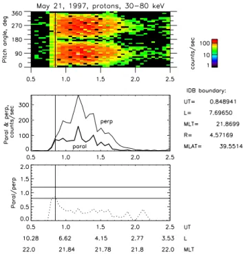
Figure 2 presents one example of Polar CAMMICE/MICS measurements on 21 May 1997 at 00:30–02:30 UT (upper panel) in counts per second for pitch angles from zero to 360◦. Polar moved inbound from the high-latitude plasma sheet to the ring current region. This gave us a unique op-portunity to search for a boundary where the isotropic pitch angle distribution changes to anisotropic at mid-altitudes, be-tween the ionosphere and equatorial plane. Because the reso-lution in local pitch angle was about 9◦, we define the parallel (to the magnetic field) count rate as a sum of counts for wide sectors of pitch angles from 0◦to 45◦and the perpendicular count rate as a sum of counts for pitch angles from 45◦ to 90◦at a given UT. They are shown in the middle panel of the Fig. 2 by thick and thin lines, respectively. The bottom panel shows the ratio between the parallel and perpendicu-lar count rates. For each pair, we determine the first point at which the ratio between the parallel and perpendicular count rates is within 0.8 and 1.2 (two horizontal lines) tailward of the maximum of the perpendicular count rate. We call this point the isotropic distribution boundary (IDB). This point is marked by a vertical line in all three panels, and it shows that the isotropization of the pitch angle distribution occurred at 00:50 UT, 21:50 MLT, L=7.7, R (radial distance)=4.6 RE
and latitude of the spacecraft was 39.5◦. The corresponding value of total magnetic field was about 400 nT.
2.3 Statistical results
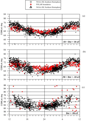
We analyzed one year (1997) of Polar measurements, when the orbit apogee was over the northern polar region. Figure 3 shows the corrected geomagnetic latitudes of the IDBs (red crosses) as a function of MLT for three ranges of the Dst
index: a) −10 nT<Dst<10 nT, b) −50 nT<Dst<−10 nT,
and c) Dst<−50 nT. The corrected geomagnetic latitudes of
the IDBs were determined using a mapping with the Tsy-ganenko T01 magnetospheric magnetic field model
(Tsyga-3.6 3.7 3.8 1 10 100 1000 10000 counts/sec -63.81 3.38 -68.32 0.56 -61.4 21.79 UT CGLat MLT 03:45:58 -64.7 22.8 May 1, 1997, NOAA 12 jP jT empty loss cone filling loss cone polar cap IB IB
Fig. 1. Example of NOAA 12 measurements on 1 May 1997
show-ing the sharp boundaries marked by vertical lines when precipitatshow-ing particle fluxes (jP) in the central part of the loss cone and locally trapped particle fluxes outside the loss cone (jT) become
compara-ble.
Fig. 2. (top panel) Polar CAMMICE/MICS measurements of
pro-ton pitch angle distributions in the energy range of 31–80 keV, (mid-dle panel) parallel (thick line) and perpendicular (thin line) count rates, and (bottom panel) the ratio between the parallel and perpen-dicular count rates for 21 May 1997, 00:30–02:30 UT. The position of IDB is marked by a vertical line at all three panels.
nenko, 2002a,b). The input parameters for each IDB obser-vation, interplanetary magnetic field and solar wind dynamic pressure, were obtained from the WIND spacecraft. Figure 3 also presents the statistical positions of isotropic boundaries for protons with an energy range of 30–80 keV observed on the NOAA 12 satellite during 1997 in the Northern (open tri-angles) and Southern (open circles) Hemispheres. Latitudes of the isotropic boundaries (IB) in the Southern Hemisphere are plotted as absolute values. As can be seen, the IB po-sitions in Southern and Northern Hemispheres do not differ significantly. Plotting both hemispheres was used to increase the statistics of the IB positions.
1842 N. Yu. Ganushkina et al.: Isotropy boundaries on mid- and low-altitude satellites 56 60 64 68 72 76 80 84 C G M L a t, d e g
NOAA IB, Southern Hemisphere POLAR boundaries NOAA IB, Northern Hemisphere
-10 < Dst < 10 nT 56 60 64 68 72 76 80 84 C G M Lat , deg 52 56 60 64 68 72 76 80 84 88 C G M Lat , deg 12 18 24 6 12 MLT (a) (b) (c) -50 < Dst < -10 nT Dst < -50 nT 56 60 64 68 72 76 80 84 C G M L a t, d e g
NOAA IB, southern hemisphere POLAR boundaries NOAA IB, northern hemisphere
-10 < Dst < 10 nT 56 60 64 68 72 76 80 84 C G M Lat , deg 52 56 60 64 68 72 76 80 84 88 C G M Lat , deg 12 18 24 6 12 MLT (a) (b) (c) -50 < Dst < -10 nT Dst < -50 nT
Fig. 3. MLT-dependence of corrected geomagnetic latitudes
of isotropic distribution boundaries (IDB) observed by Polar CAMMICE/MICS (red crosses), together with isotropic bound-aries (IB) observed by NOAA 12 satellites in the North-ern (open triangles) and SouthNorth-ern (open circles) Hemispheres for (a) −10 nT<Dst<10 nT, (b) −50 nT<Dst<−10 nT, and (c) Dst<−50 nT.
The obtained statistical properties of IDBs are quite sim-ilar to those of the IBs (Sergeev and Gvozdevsky, 1995). These boundaries (IDBs and IBs) were observed at all MLTs. There exists a day-night asymmetry with the night-side boundaries being at lower latitudes than those on the dayside. An increase of activity (decrease in the Dst index)
leads to an equatorward shift of boundaries at all MLTs. At the same time, there exists a small difference between av-erage IDB and IB latitudes which is most pronounced on the nightside and on the dayside. For the quiet conditions with −10 nT<Dst<10 nT IDBs are observed in the
latitudi-nal range of 65◦−69◦on the nightside and 69◦−73◦on the dayside. IDBs are observed below 64◦(60◦) on the night-side and 68◦(65◦) on the dayside for −50 nT<Dst<−10 nT
(Dst<−50 nT). The IDB positions become more scattered
and occupy a larger latitudinal interval at a given MLT than the IBs. A very scattered pattern is observed during disturbed conditions when Dst<−50 nT. For all three Dst ranges IBs
are observed at lower latitudes than IDBs on the nightside.
2 0 -2 -4 -6 -8 -10 Xgsm, Re -4 -2 0 2 4 6 Zg sm , R e May 21, 1997, Dst=-6 nT 2 0 -2 -4 -6 -8 -10 Xgsm, Re -2 0 2 4 6 Y g sm , R e
Polar IDB: 00:48:45 UT, -69.10 lat, 21.9 MLT
DMSP b2i: 00:43:39 UT, -68.80 lat, 22.1 MLT
2 0 -2 -4 -6 -8 Xgsm, Re -2 0 2 4 Zg sm , R e May 1, 1997, Dst=-16 nT 2 0 -2 -4 -6 -8 Xgsm, Re -3 -2 -1 0 1 2 3 Y g sm , R e
Polar IDB: 03:30:00 UT, -65.40 lat, 22.8 MLT
NOAA IB: 03:45:58 UT, -64.70 lat, 22.6 MLT
2 0 -2 -4 -6 Xgsm, Re -4 -2 0 2 4 Zg sm , R e May 28, 1997, Dst=-24 nT 2 0 -2 -4 -6 Xgsm, Re -2 0 2 4 6 8 Y g sm , R e
Polar IDB: 09:30:00 UT, -66.0 lat, 20.5 MLT
NOAA IB: 09:05:12 UT, -66.450 lat, 20.09 MLT
2 0 -2 -4 -6 -8 Xgsm, Re -3 -2 -1 0 1 2 Zg sm , R e October 10, 1997, Dst=-49 nT 2 0 -2 -4 -6 -8 Xgsm, Re -3 -2 -1 0 1 2 Y g sm, R e
Polar IDB: 10:51:20 UT, -63.300 lat, 0.2 MLT
DMSP b2i: 10:56:46 UT, -63.20 lat, 23.7 MLT
(a)
(b)
(c)
(d)
Fig. 4. Noon-midnight meridian (left panels) and equatorial plane
(right panels) projections of the magnetic field lines correspond-ing to DMSP or NOAA (black lines) and Polar (red line) locations, when the conjugate boundaries were observed at Polar and DMSP on (a) 21 May 1997 and (d) 10 October 1997, and at Polar and NOAA on (b) 1 May 1997 and (c) 28 May 1997. The thick red cross shows the Polar location.
3 Comparison of mid-altitude and low-altitude conju-gate observations
In addition to the comparison of statistical results on mid-altitude IDBs as observed by Polar and low-mid-altitude IBs ob-served by NOAA, we searched for several conjugate obser-vations by Polar and NOAA, and Polar and DMSP. Like the NOAA spacecraft, the DMSP satellites have a 101-min Sun-synchronous, near-polar orbit at 830 km altitude. Using the observations made in 1997, for both Polar and NOAA, and Polar and DMSP, we searched for cases when NOAA and DMSP observations and Polar observations were within 30 min of each other (1UT<30 min) and in the same local time sector (1MLT<30 min). For Polar and DMSP conjunc-tions, we used IDBs at Polar and the b2i boundary (the en-ergetic ion precipitation flux peak) at DMSP which corre-sponds well to the proton isotropic precipitating boundary at 30 keV energy (Newell et al., 1998).
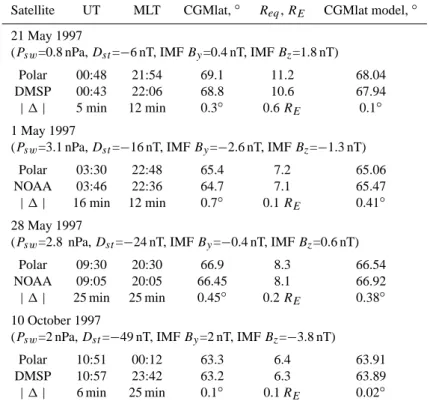
Table 1. Positions of Polar, NOAA and DMSP satellites for conjugate events, together with solar wind parameters, Dst index, and
corre-sponding magnetic field line parameters.
Satellite UT MLT CGMlat,◦ Req, RE CGMlat model,◦
21 May 1997
(Psw=0.8 nPa, Dst=−6 nT, IMF By=0.4 nT, IMF Bz=1.8 nT)
Polar 00:48 21:54 69.1 11.2 68.04
DMSP 00:43 22:06 68.8 10.6 67.94
|1 | 5 min 12 min 0.3◦ 0.6 RE 0.1◦
1 May 1997
(Psw=3.1 nPa, Dst=−16 nT, IMF By=−2.6 nT, IMF Bz=−1.3 nT)
Polar 03:30 22:48 65.4 7.2 65.06
NOAA 03:46 22:36 64.7 7.1 65.47
|1 | 16 min 12 min 0.7◦ 0.1 RE 0.41◦
28 May 1997
(Psw=2.8 nPa, Dst=−24 nT, IMF By=−0.4 nT, IMF Bz=0.6 nT)
Polar 09:30 20:30 66.9 8.3 66.54
NOAA 09:05 20:05 66.45 8.1 66.92
|1 | 25 min 25 min 0.45◦ 0.2 RE 0.38◦
10 October 1997
(Psw=2 nPa, Dst=−49 nT, IMF By=2 nT, IMF Bz=−3.8 nT)
Polar 10:51 00:12 63.3 6.4 63.91
DMSP 10:57 23:42 63.2 6.3 63.89
|1 | 6 min 25 min 0.1◦ 0.1 RE 0.02◦
Figure 4 presents two selected conjunctions between Polar and DMSP for a) 21 May 1997 and d) 10 October 1997, and two between Polar and NOAA for b) 1 May 1997 and c) 28 May 1997. These cases were selected to cover the interval of activity conditions from quiet with Dst=−6 nT on 21 May
1997, to disturbed with Dst=−49 nT on 10 October 1997.
Noon-midnight meridian (left panels) and equatorial plane (right panels) projections of the magnetic field lines corre-sponding to DMSP or NOAA (black lines) and Polar (red line) locations, when the isotropy boundaries were observed, are shown. We used the Tsyganenko T01 model (Tsyga-nenko, 2002a,b) with the observed solar wind conditions and Dstindex as input parameters for the magnetic field
calcula-tions. The thick red cross shows the Polar location.
Table 1 presents, together with corresponding IMF and so-lar wind parameters and Dst indices, the UTs and MLTS of
the positions of IDBs, IBs and b2i boundaries observed by Polar, NOAA and DMSP, respectively. The corrected ge-omagnetic latitudes and equatorial distances for correspond-ing magnetic field lines calculated uscorrespond-ing the Tsyganenko T01 model with the observed parameters for the four selected conjugate events are also shown.
For all four cases, independent of the activity conditions, the differences in latitudes of the observed IDBs at Polar and IB at NOAA and b2i at DMSP were rather small, less than 1◦, with a maximum difference of 0.7◦on 1 May 1997, when Dst was equal to −16 nT. The difference in equatorial radial
distance was also small, reaching 0.6 RE on 21 May 1997,
when Dst was about −6 nT.
We also computed the model locations of the expected isotropy boundaries by finding the magnetic field lines (at MLTs of Polar, NOAA and DMSP) on which the criterion of Rc/ρ=8 is fulfilled (Sergeev and Tsyganenko, 1982). For
Po-lar data we are restricted by 9◦in pitch angle and an 8-energy level resolution for the count rates. This seriously limits our possibility to gain information about the detailed structure of the distribution function in this rather limited energy range of 30–80 keV. In our model calculations we used the proton energy of 30 keV. We assumed that the distribution is close to Maxwellian and thus the maximum will be for lower en-ergies. The larmor radius for low energy particles will be smaller, and hence the ratio Rc/ρ will be larger. Making
calculations for the energy of 30 keV, we find the maximum Rc/ρvalues for the given energy range of 30–80 keV.
The latitudes of model and observed boundaries, shown in the last column in Table 1, are quite close to each other. The differences in latitudes between the model boundaries for conjugate Polar, NOAA and DMSP observations are also small, not exceeding 0.4◦.
4 Discussion
We determined the locations of mid-altitude isotropic dis-tribution boundaries (IDB), where anisotropic pitch an-gle distributions (perpendicular flux dominating) change to isotropic distributions using Polar CAMMICE MICS proton data and compared them to the low-altitude isotropic
bound-1844 N. Yu. Ganushkina et al.: Isotropy boundaries on mid- and low-altitude satellites 56 60 64 68 72 76 80 84 C G M L a t, d e g -10 < Dst < 10 nT 56 60 64 68 72 76 80 84 C G M Lat , deg 52 56 60 64 68 72 76 80 84 88 C G M Lat , deg 12 18 24 6 12 MLT (a) (b) (c) -50 < Dst < -10 nT Dst < -50 nT
Polar fit: cgmlat=69.536-2.015 cos(π/12(MLT-23.11))
NOAA fit: cgmlat=69.674-4.595 cos(π/12(MLT-23.37))
Polar fit: cgmlat=68.317-2.24 cos(π/12(MLT-22.95))
NOAA fit: cgmlat=68.06-4.55 cos(π/12(MLT-23.09))
Polar fit: cgmlat=66.76-5.69 cos(π/12(MLT-20.64))
NOAA fit: cgmlat=65.795-4.287cos(π/12(MLT-22.8))
Fig. 5. Lat (MLT )=A0−A1cos(π(MLT −MLT0)/12)
ap-proximation for Polar IDB statistics (red curves) and NOAA IB statistics (black curves) (a) −10 nT<Dst<10 nT, (b) −50 nT<Dst<−10 nT, and (c) Dst<−50 nT. Standard error
means are shown by open red triangles for Polar data and by open black diamonds for NOAA data.
aries (IB) observed by NOAA and DMSP satellites dur-ing 1997. The fact that the mid-altitude IDB and low-altitude IB and b2i boundaries were found on very close field lines (Fig. 4) suggests that they are associated with the same isotropization mechanism. Simultaneous observa-tions of isotropization signatures at low- and mid-altitudes is a strong argument supporting the mechanism of filling the ionospheric loss cone by pitch angle scattering due to viola-tion of first adiabatic invariant while crossing the tail current sheet.
Statistical CGLat-MLT dependencies of the IDB and IB positions were found to be very similar, but systematic dif-ferences in their latitudes exist most pronounced on the nightside and on the dayside (Fig. 3). Following Sergeev and Gvozdevsky (1995) we fitted the statistical observations by Polar and NOAA using a simple cosine approximation Lat (MLT)=A0−A1cos(π (MLT−MLT0)/12), where A0 is the average latitude, A1 is the amplitude and MLT0 is the phase shift. Figure 5 shows the fits for Polar IDB statis-tics (red curves) and NOAA IB statisstatis-tics (black curves) for (a) −10 nT<Dst<10 nT, (b) −50 nT<Dst<−10 nT, and (c)
Dst<−50 nT. Standard error means are shown by open red
triangles for Polar and by open black diamonds for NOAA.
For all three cases IDBs are observed at higher latitudes on the nightside and at lower latitudes on the dayside than IBs. The phase shift towards the dusk exists for both boundaries (increasing with the activity increase) and is larger for Po-lar IDBs than for NOAA IBs, simiPo-lar to that previously re-ported for isotropic and b2i boundaries (Newell et al., 1998) and proton auroras (Donovan et al., 2003). The sparse MLT coverage, however, does not allow for a more detailed inves-tigation of this feature in our data set.
Although we compared directly the locations of IBs ob-served by low-altitude NOAA satellite and IDBs obob-served by mid-altitude Polar satellite, it should be clearly mentioned that these two boundaries have a different definition. Low-altitude NOAA MEPED detectors look radially outward and perpendicular to the satellite velocity vector and measure only precipitating and locally mirroring particles. In these data, particles seen in the two directions have very small pitch angle separation at the equator: particles with 10◦and
80◦pitch angles detected by NOAA will have only 0.31◦and 1.78◦pitch angles at the equator (∼9 RE). The low-altitude
isotropic boundary (IB) reflects the transition from the empty loss cone to the isotropically filled loss cone, therefore, it characterizes the pitch angle change during one traversal of the equatorial current sheet. However, the required pitch an-gle change is very small, of the order of the loss-cone size in the current sheet center, i.e. about 1–2◦.
We define the IDB at Polar not in terms of filling the loss cone but as a boundary where the parallel count rate (sum of counts for pitch angles from 0◦to 45◦) and the perpendicular count rate (sum of counts for pitch angles from 45◦to 90◦) become comparable (Fig. 2). Polar IDB is observed at mid-altitudes (total magnetic field is about 300–400 nT), where a large portion of the equatorial plasma distribution is present. IDB characterizes a change in the entire distribution, rather than a change in a small part near the small loss cone like the IB. This change is formed by the interaction of two com-petitive processes. One of them is pitch angle scattering due to the non-adiabatic motion, which isotropizes the distribu-tion. The other process is the inward convection in the in-ner magnetosphere, which creates a pancake-like anisotropy due to the dominating betatron acceleration. For that reason, one would expect the IDB at larger distances than the IB on the nightside, where the pitch angle scattering is presumably stronger, which was indeed the case.
To have an idea where in the magnetosphere pitch angle scattering can occur, we integrated particle trajectories with a standard method of 4th order Runge-Kutta scheme in the T01 magnetic field model with quiet-time parameters. Figure 6 illustrates the results for protons with 30 keV. It shows the Rc/ρ-dependence of the phase-averaged pitch angle changes
after one crossing of the field reversal region at the midnight meridian. Each point is the average of 18 trajectories, which differ by initial phase. Initial pitch angles varied from 0◦to 35◦(with 5◦step), whereas the initial phase for each initial pitch angle varied from 0◦to 360◦(in 20◦steps). The pitch-angles are reduced to the equator.
3 4 5 6 7 8 9 10 Rc/ρ 0.1 1 10 -α, de gr ee
Fig. 6. Rc/ρ–dependence of the phase-averaged pitch angle
changes (pitch angles reduced to the magnetic equator) after one crossing of the field reversal region calculated by tracing the 30-keV protons in the T01 magnetic field at midnight meridian. Initial pitch angles varied from 0◦to 35◦(with 5◦step), whereas the ini-tial phase for each iniini-tial pitch angle varied from 0◦to 360◦(in 20◦ steps).
Similar to previous computations (Sergeev and Tsyga-nenko, 1982; Delcourt et al., 1996), the pitch angle change is small for large Rc/ρ≥10 (of the order of the loss-cone size
∼0.7◦, when Rc/ρ∼8) and strongly increases with further
decreasing of Rc/ρ. When Rc/ρfalls below 5–6, the
scat-tering increases by a factor of 2.5 and it quickly isotropizes the distribution. This is the location where the IDB is ex-pected to be observed on the nightside. The statistical obser-vations of IDBs at higher latitudes than IBs on the nightside qualitatively agree with this picture.
Having computed the T01 model for each Polar observa-tion point, we mapped the observed IDB locaobserva-tions to the equatorial plane in order to check the Rc/ρvalues. As shown
in Fig. 4, using the criterion Rc/ρ=8 to determine the
lati-tudes of isotropy boundaries predicted by the magnetic field model the results differed from the observed ones by about 1–2◦. An obvious reason for that is the error in the model magnetic field, which may be evaluated by comparison with the observed magnetic field value.
The position of the modelled IDB can be influenced by the choice of the energy for which the calculations of Rc/ρ are
made, the value of Rc/ρ itself, which is selected as a
cri-teria for the pitch angle scattering and the accuracy of the magnetic field model. We can estimate the differences com-ing from energy or Rc/ρ changing. As simple calculations
have shown, for 10 October 1997 event (Fig. 4d) for pro-tons with 30 keV energy the model IDB latitude is 63.9◦for Rc/ρ=8 and 64.16◦for Rc/ρ=6. For protons with 80 keV
en-ergy the latitude is equal to 63.44◦Rc/ρ=8. Thus, changing
the energy or Rc/ρ value does not produce big changes in
the model IDBs and does not influence our conclusions. It is more difficult to estimate properly the error coming from the magnetic field model. When we have a good correspondence
-0.5 -0.4 -0.3 -0.2 -0.1 0 0.1 0.2 0.3 0.4 0.5 ∆B=[(Bmod - Bobs)/Bobs]ext 0.1 1 10 100 Rc /ρ -10 < Dst < 10 nT -50 < Dst < -10 nT -150 < Dst < -50 nT ln(Y) = -2.6X + 1.7 04 < MLT < 20
Fig. 7. Dependence of the computed values of Rc/ρ on
the accuracy parameter 1B=BT01−Bobs
Bobs corresponding to the
Polar IDB observations on the nightside (04<MLT <20) for
−10 nT<Dst<10 nT (green triangles), −50 nT<Dst<−10 nT (red
triangles) and −150 nT<Dst<−50 nT (blue crosses). Here the
in-terval of 1B from −0.5 to 0.5 is shown as it represents good accu-racy. The red line represents the fit ln(Rc/ρ)=−2.6 1B+1.7.
between the observed and modelled magnetic field at the Po-lar location, we do not know if the model is accurate at the equator where we estimate the field line curvature. For this, the close location of the magnetic field lines corresponding to observations of IDB on Polar, IB on NOAA, and b2i on DMSP, is an indicator of the model’s sufficient accuracy.
To check further the accuracy of the magnetic field model used in the present study, for each Polar observation of IDB on the nightside (04<MLT <20) we computed a rel-ative error parameter 1B=BT01−Bobs
Bobs , where BT01is the
ex-ternal magnetic field calculated using the Tsyganenko T01 model with the observed parameters and Bobs is the
ob-served external magnetic field (internal magnetic field given by IGRF model was subtracted from the observed mag-netic field) given by the Polar MFE instrument. Then, for each Polar position we computed the value of Rc/ρ
using the T01 model, assuming the proton energy to be 30 keV. Figure 7 shows the dependence of the computed values of Rc/ρ on the accuracy parameter 1B
correspond-ing to the Polar IDB observations for −10 nT<Dst<10 nT
(green triangles), −50 nT<Dst<−10 nT (red triangles) and
−150 nT<Dst<−50 nT (blue crosses). Here we show the
interval of 1B from −0.5 to 0.5. It can be seen that for all Dst ranges the computed Rc/ρincreases with 1B decrease.
When 1B<0, then BT01<Bobs. This means that the model
underestimates the tail currents, and the model magnetic field line is less stretched than the observed one. The model Rc/ρ
value is larger than needed for scattering, and scattering oc-curs further tailward. When 1B>0, then BT01>Bobs, and
1846 N. Yu. Ganushkina et al.: Isotropy boundaries on mid- and low-altitude satellites the model magnetic field lines are too stretched. The
scatter-ing occurs at larger Rc/ρvalues than given by the model.
In Fig. 7 the red line represents the fit ln(Rc/ρ)=−2.6
1B+1.7. The scattering criterion is determined at the inter-section of this fit, and is about 6, and 1B=0 . The obtained value of Rc/ρ agrees well with our expectations based on
the strength of pitch angle scattering and confirms that the regular mechanism of non-adiabatic particle scattering in the current sheet is responsible for maintaining the isotropic pro-ton distribution functions on the nightside. It also supports the conclusions made by West et al. (1978) from two in-situ comparisons of theoretical and observed boundaries. Taking into account the consistency between IDB and IB boundary locations at dusk and dawn (where convection lines go along the boundary and where convection plays a minor role in the restoring the anisotropy), one may also expand this conclu-sion to the dusk and dawn portions of the IDB distribution.
On the other hand, according to Fig. 6, at Rc/ρ=6 the
changes in the particle pitch angle can be as large as several degrees, which confirms our speculations concerning the re-quirement of stronger scattering for producing IDBs seen at Polar. It is also necessary to mention that the magnetospheric magnetic field models used for magnetic field mapping usu-ally overestimate the thickness of the tail current sheet, which can lead to even smaller values of Rc/ρthan 6.
As was mentioned above, calculations were made for the energy of 30 keV, assuming the distribution to be close to Maxwellian witha maximum at lower energies. The chang-ing in the energy from the lower limit of the energy range (30 keV) to the upper limit (80 keV) will result in the shift of the corresponding fit (Fig. 7), and a lower intersection of this fit and 1B=0, to lower Rc/ρvalues, but will not lead to
a dramatic change in the expected trend for IDB points and our conclusions.
Although we discussed only the nightside isotropic distri-bution boundaries, we may expect the same physics to be valid for the dayside boundaries. However, it is more diffi-cult to obtain experimental confirmation and to control the mapping errors in that region. The field lines here expe-rience strong 3-D deformations: two field lines which are closeby may map to very different domains in the equatorial plane. For example, the field line coming from near the cusp can map to either near the dayside magnetopause (where the magnetic field is strong and Rc/ρ is very large) or to near
the magnetopause in the far magnetotail (where the magnetic field and Rc/ρare very small). Also, these deformations are
very sensitive to the intensity and distribution of the field-aligned currents. In general, this region is described with less confidence in the magnetospheric models. This does not al-low us to interpret the dayside observations in the same way as we did for the nightside.
When finding the IDBs observed by Polar, we considered only local measurements, not following the pitch-angle dis-tribution evolution and not mapping to the equatorial plane. Also a comparison with DMSP was made using local mea-surements. At the same time, the particles drift so that the measured distributions at Polar and DMSP may be
differ-ent. Tracing of particle trajectories in realistic magnetic field models and comparison with pitch angle observations is our future task.
The isotropization of the distribution at Polar does not nec-essarily mean isotropic precipitation of ions at low-altitudes at the same time; other local mechanisms of isotropization at Polar altitudes could well be active. The role of wave-particle interactions in the process of isotropization at different alti-tudes needs to be investigated further in a future study.
5 Conclusions
In this paper we confirm and extend previous results describ-ing and explaindescrib-ing the transition from anisotropic proton dis-tributions in the near-Earth tail to the isotropic disdis-tributions in the nightside plasma sheet.
We showed that two different boundaries (IB, related to the isotropic filling of the loss cone by non-adiabatic pitch angle scattering, and IDB, characterizing the pitch angle dis-tributions in the near-equatorial magnetosphere) stay on the neighboring field lines and display similar CGLatitide-MLT distributions and similar activity dependence. Furthermore, introducing a procedure to control the difference between ob-served and the model magnetic field we were able to reduce a large scatter in mapped equatorial parameters and to con-clude that the isotropic distribution boundary (IDB) lies in the region where Rc/ρ∼6. In this region the pitch angle
scat-tering is strong enough (>10◦for one current sheet crossing
by a test particle). We, therefore, conclude that the scattering in the large field-line curvature regions of the nightside cur-rent sheet is the main mechanism producing isotropization for the main portion of proton population in the tail current sheet. This mechanism controls the observed positions of the IB and IDB boundaries and, therefore, can be probed with observations of these isotropy boundaries.
Acknowledgements. We would like to thank K. Ogilvie and R.
Lep-ping for the use of WIND data, C. Russell for Polar MFE data ob-tained from the Coordinated Data Analysis Web (CDAWeb) and World Data Center C2 for Geomagnetism, Kyoto, for the provi-sional Dst indices data. We thank P. Newell for the DMSP b2i
boundaries available from JHU/APL website. The NOAA data were obtained from WDC for Aurora, NIPR, Tokyo, Japan. This work was supported by Academy of Finland. The work of M. Kubyshk-ina, V. Sergeev and E. Lvova was supported by RFBR grant 04-05-64932. The work of T. Yahnina and A. Yahnin was supported by the Division of Physical Sciences of Russian Academy of Science via the program DPS-18.
Topical Editor in chief thanks L. Zelenyi and F. S¨oraas for their help in evaluating this paper.
References
Alfv´en, H. and F¨althammar, C. G.: Cosmic Electrodynamics, Fun-damental Principles, (2nd edition), Clarendon, Oxford, 1963. Ashour-Abdalla, M. and Kennel, C. F.: Diffuse auroral
Birmingham, T. J.: Pitch angle diffusion in the Jovian magnetodisc, J. Geophys. Res., 89, 2699–2707, 1984.
B¨uchner, J. and Zelenyi, L. M.: Chaotization of the electron motion as the cause of an internal magnetotail instability and substorm onset, J. Geophys. Res., 92, 13 456–13 466, 1987.
Delcourt, D. C., Sauvaud, J.-A., Martin, Jr., R. F. and Moore, T. E.: On the nonadiabatic precipitation of ions from the near-earth plasma sheet, J. Geophys. Res., 101, 17 409–17 418, 1996. De Michelis, P., Daglis, I. A., and Consolini, G.: An average image
of proton plasma pressure and of current systems in the equato-rial plane derived from AMPTE/CCE-CHEM measurements, J. Geophys. Res., 104, 28 615–28 624, 1999.
Donovan, E. F., Jackel, B. J., and Voronkov, I., et al.: Ground-based optical determination of the b2i boundary: A basis for an opti-cal MT-index, J. Geophys. Res., 108, SMP 10-1, CiteID 1115, doi:10.1029/2001JA009198, 2003.
Hill, V. D., Evans, D. S. and Sauer, H. H.: TIROS/NOAA satel-lites space environment monitor, Archive tape documentation, NOAA Tech. Mem. ERL SEL-71, 50, Environs. Res. Lab., Boul-der, 1985.
Hultqvist, B.: The hot ion component of the magnetospheric plasma and some relations to the electron component: Observations and physical implications, Space Sci. Rev., 23, 581–675, 1979. Imhof, W. L., Reagan, J. B. and Gaines, E. E.: Fine-scale spatial in
the pitch angle distributions of energetic particles near the mid-night trapping boundary, J. Geophys. Res., 82, 5215–5221, 1977. Imhof, W. L., Reagan, J. B., and Gaines, E. E.: Studies of the sharply defined L dependent energy threshold for isotropy at the midnight trapping boundary, J. Geophys. Res., 84, 6371–6384, 1979.
Lui, A. T. Y. and Hamilton, D. C.: Radial profiles of quiet time mag-netospheric parameters, J. Geophys. Res., 97, 19 325–19 332, 1992.
Milillo, A., Orsini, S., Delcourt, D. C., et al.: Empirical model of proton fluxes in the equatorial inner magnetosphere: 2. Properties and applications, J. Geophys. Res., 108, 1165, doi:10.1029/2002JA009581, 2003.
Newell, P. T., Sergeev, V. A., Bikkuzina, G. R. and Wing, S.: Char-acterizing the state of the magnetosphere: Testing the ion pre-cipitation maxima latitude (b2i) and the ion isotropy boundary, J. Geophys. Res., 103, 4739–4745, 1998.
Russell, C. T., Snare, R. C., Means, J. D., et al.: The GGS/Polar Magnetic Fields Investigation, Space Sci. Rev., 71, 563–582, 1995.
Sergeev, V. A. and Gvozdevsky, B. B.: MT-index − A possible new index to characterize the magnetic configuration of magnetotail, Ann. Geophys., 13, 1093–1103, 1995,
SRef-ID: 1432-0576/ag/1995-13-1093.
Sergeev, V. A., Malkov, M., and Mursula, K.: Testing the isotropic boundary algorithm method to evaluate the magnetic field con-figuration in the tail, J. Geophys. Res., 98, 7609–7620, 1993. Sergeev, V. A., Sazhina, E. M., Tsyganenko, N. A., Lundblad,
J. A., and Soraas, F.: Pitch-angle scattering of energetic pro-tons in the magnetotail current sheet as the dominant source of their isotropic precipitation into the nightside ionosphere, Planet. Space Sci., 31, 1147–1155, 1983.
Sergeev, V. A. and Tsyganenko, N. A.: Energetic particle losses and trapping boundaries as deduced from calculations with a realistic magnetic field model, Planet. Space Sci., 30, 999–1006, 1982. Stiles, G. S., Hones, Jr., E. W., Bame, S. J., and Asbridge, J. R.:
Plasma sheet pressure anisotropies, J. Geophys. Res., 83, 3166– 3172, 1978.
Søraas, F.: ESRO IA/B observations at high latitudes of trapped and precipitating protons with energies above 100 keV, in: Earths magnetospheric processes, edited by: B. M. McCormac, 121– 132, D. Reidel, Norwell, Mass., 1972.
Taylor, H. E. and Hastie, R. J.: Nonadiabatic behavior of radiation belt particles, Cosmic Electrodyn., 2, 211–223, 1971.
Tsyganenko, N. A.: Pitch-angle scattering of energetic particle in the current sheet of the magnetospheric tail and stationary distri-bution functions, Planet. Space Sci., 30, 433–437, 1982. Tsyganenko, N. A.: A model of the near magnetosphere
with a dawn-dusk asymmetry: 1. Mathematical struc-ture, J. Geophys. Res., 107, SMP 12-1, CiteID 1179, doi:10.1029/2001JA0002192001, 2002a.
Tsyganenko, N. A.: A model of the near magnetosphere with a dawn-dusk asymmetry: 2. Parameterization and fitting to ob-servations, J. Geophys. Res., 107, SMP 10-1, CiteID 1176, doi:10.1029/2001JA000220, 2002b.
Wagner, J. S., Kan, J. R., and Akasofu, S.-I.: Particle dynamics in the plasma sheet, J. Geophys. Res., 84, 891–897, 1979. West, H. I., Jr., Buck, R. M., and Kivelson, M. G.: On the
configu-ration of the magnetotail near midnight during quiet and weakly disturbed periods: State of the magnetosphere, J. Geophys. Res., 83, 3805–3817, 1978.
Wilken, B., Weiss, W., Hall, D., Grande, M., Soraas, F., and Fennell, J. F.: Magnetospheric ion composition spectrometer on board the CRRES spacecraft, J. Spacecr. Rockets, 29, 585–591, 1992. Yahnina T. A., Yahnin, A. G., Kangas, J., et al.: Energetic particle
counterparts for geomagnetic pulsations of Pc1 and IPDP types, Ann. Geophys., 21, 2281–2292, 2003,
SRef-ID: 1432-0576/ag/2003-21-2281.
Young, S. L., Denton, R. E., Anderson, B. J., and Hudson, M. K.: Empirical model for µ scattering caused by field line cur-vature in a realistic magnetosphere, J. Geophys. Res., 107, 1069, doi:10.1029/2000JA000294, 2002.