HAL Id: hal-00318827
https://hal.archives-ouvertes.fr/hal-00318827
Submitted on 1 Jan 2002
HAL is a multi-disciplinary open access
archive for the deposit and dissemination of
sci-entific research documents, whether they are
pub-lished or not. The documents may come from
teaching and research institutions in France or
abroad, or from public or private research centers.
L’archive ouverte pluridisciplinaire HAL, est
destinée au dépôt et à la diffusion de documents
scientifiques de niveau recherche, publiés ou non,
émanant des établissements d’enseignement et de
recherche français ou étrangers, des laboratoires
publics ou privés.
observations from the arctic to equator and comparisons
with the HRDI measurements and the GSWM
modelling results
Y. Luo, A. H. Manson, C. E. Meek, C. K. Meyer, M. D. Burrage, D. C. Fritts,
C. M. Hall, W. K. Hocking, J. Macdougall, D. M. Riggin, et al.
To cite this version:
Y. Luo, A. H. Manson, C. E. Meek, C. K. Meyer, M. D. Burrage, et al.. The 16-day planetary waves:
multi-MF radar observations from the arctic to equator and comparisons with the HRDI measurements
and the GSWM modelling results. Annales Geophysicae, European Geosciences Union, 2002, 20 (5),
pp.691-709. �hal-00318827�
Geophysicae
The 16-day planetary waves: multi-MF radar observations from the
arctic to equator and comparisons with the HRDI measurements
and the GSWM modelling results
Y. Luo1, *, A. H. Manson1, C. E. Meek1, C. K. Meyer2, M. D. Burrage3, **, D. C. Fritts2, C. M. Hall4, W. K. Hocking5, J. MacDougall5, D. M. Riggin2, and R. A. Vincent6
1Institute of Space and Atmospheric Studies, University of Saskatchewan, Canada 2Colorado Research Associates, Boulder, USA
3Space Physics Research Laboratory, University of Michigan, Ann Arbor, USA 4Tromsø Geophysical Observatory, University of Tromsø, Norway
5Department of Physics and Astronomy, University of Western Ontario, Canada 6Department of Physics and Mathematical Physics, University of Adelaide, Australia *now at: Canada Centre for Remote Sensing, Ottawa, Canada
**M. Burrage died tragically on 10 October 1999, and we dedicate this paper to his memory.
Received: 27 August 2001 – Revised: 27 December 2001 – Accepted: 8 January 2002
Abstract. The mesospheric and lower thermospheric (MLT) winds (60–100 km) obtained by multiple MF radars, lo-cated from the arctic to equator at Tromsø (70◦N, 19◦E), Saskatoon (52◦N, 107◦W), London (43◦N, 81◦W), Hawaii
(21◦N, 157◦W) and Christmas Island (2◦N, 157◦W),
re-spectively, are used to study the planetary-scale 16-day waves. Based on the simultaneous observations (1993/1994), the variabilities of the wave amplitudes, periods and phases are derived. At mid- and high-latitude locations the 16-day waves are usually pervasive in the winter-centred seasons (October through March), with the amplitude gradually de-creasing with height. From the subtropical location to the equator, the summer wave activities become strong at some particular altitude where the inter-hemisphere wave ducts possibly allow for the leakage of the wave from the other hemispheric winter. The observational results are in good agreement with the theoretical conclusion that, for slowly westward-traveling waves, such as the 16-day wave, verti-cal propagation is permitted only in an eastward background flow of moderate speed which is present in the winter hemi-sphere. The wave period also varies with height and time in a range of about 12–24 days. The wave latitudinal dif-ferences and the vertical structures are compared with the Global Scale Wave Model (GSWM) for the winter situation. Although their amplitude variations and profiles have a sim-ilar tendency, the discrepancies are considerable. For exam-ple, the maximum zonal amplitude occurs around 40◦N for radar but 30◦N for the model. The phase differences between sites due to the latitudinal effect are basically consistent with the model prediction of equatorward phase-propagation. The global 16-day waves at 95 km from the HRDI wind
measure-Correspondence to: Y. Luo ([email protected])
ments during 1992 through 1995 are also displayed. Again, the wave is a winter dominant phenomenon with strong amplitude around the 40–60◦ latitude-band on both hemi-spheres.
Key words. Meteorology and atmospheric dynamics – waves and tides – middle atmosphere dynamics – thermo-spheric dynamics
1 Introduction
The studies of planetary waves (PW) in the mesosphere and lower thermosphere (MLT), based upon a variety of observa-tions from ground-based and/or satellite-borne systems, have been reported widely during the past several decades (Muller et al., 1972; Manson et al., 1978; Tsuda et al., 1988; Vin-cent, 1990; Meek et al., 1996; Palo et al., 1996; Fritts et al., 1999; Clark et al., 2002). It has been proposed that many of the PWs appearing in the MLT region are not excited in situ but have propagated from lower atmospheric sources, i.e. those PWs (or Rossby waves) observed in the troposphere and stratosphere. Theoretical studies and numerical models have indicated that the upward propagation of PWs is possi-ble from the stratosphere up to the mesopause region under certain atmospheric conditions (Charney and Drazin, 1961; Dickinson, 1968; Salby, 1981a, b; Forbes et al., 1995a).
From solutions of Laplace’s tidal equation one can obtain a series of classical normal modes denoted by (s, n − s) for westward propagating Rossby waves; here, s is the zonal wave number, and n is the meridional index derived from the subscripts of Hough functions. The MLT PWs are usu-ally observed with periods around 2, 5–7, 8–10 and 12–22
days. They are comparable with those modes of (3, 0), (1, 1), (1, 2) and (1, 3), respectively, provided that in realis-tic atmospheres, these modes’ eigenperiods of 2, 5, 8.3 and 12.5 days may be modified due to Doppler shifting by the non-zero background flow (Forbes, 1995b). The pioneering work regarding the upward propagation of PW by Charney and Drazin (1961) showed that the index of refraction for the stationary PW depends primarily on the distribution of the mean zonal wind with height. Energy is trapped/reflected in regions where the zonal winds are westward or strongly eastward. Although their conclusion was drawn from a sta-tionary wave consideration, it is still applicable for travelling waves after replacing the zero phase velocity with a suitable value, the intrinsic phase velocity. Therefore, the vertical wave propagation of the various normal modes is weakly or strongly sensitive to the background zonal flow depending upon the wave’s phase velocity. When the westward phase speed of a mode is less than or equal to the westward mean wind speed, the propagation will be blocked. Since the 16-day wave has a small westward phase speed, numerical sim-ulations indicate that it will be trapped in the strong west-ward flow of the summer stratosphere and can only propagate directly up into the MLT region through the winter strato-spheric eastward jet.
Due to the sensitivity of the 16-day wave to the back-ground wind and/or the wave variability in space and time, and also due to the requirement of high quality data sets, i.e. longer duration, better continuity and higher velocity resolution, the 16-day waves in the MLT region have not been studied substantially until recent years. Using an MST (mesosphere-stratosphere-troposphere) radar, Williams and Avery (1992) studied the 16-day wave of the year 1984 at Poker Flat (65◦N, 147◦W), Alaska. Consistent with the
above theoretical discussion, in the stratosphere, the 16-day wave had maximum amplitudes in winter, but contrarily, in the mesosphere, it was maximum in summer around the mesopause (85 km). They suggested two origins for the lat-ter situation. For the first possibility, the 16-day wave gen-erated in the winter hemisphere propagates vertically and then crosses the equator toward the summer pole follow-ing the eastward mean wind fields of the mesopause region. The second is that the gravity waves (GW) in the summer troposphere are modulated by the 16-day waves there and then propagate upward and deposit momentum, due to wave breaking or viscous dissipation, in the mesosphere in a 16-day cycle. Forbes et al. (1995a) analyzed the 1979 win-ter mesopause-region winds measured at Obninsk (54◦N,
38◦E), Russia and Saskatoon. A 16-day oscillation of the
order of 10 m/s, with zonal wave number 1, was manifested when a large oscillation of this type was observed in the tro-posphere and stratosphere. They also performed numerical simulations confirming the direct upward propagation into the MLT region of the 16-day wave under a suitable January wind field, also showing a ducting channel enabling inter-hemispheric penetration of that 16-day wave. Another nu-merical model (Miyoshi, 1999) showed that the penetration of the 16-day wave from the winter hemisphere to the
sum-mer hemisphere occurs near the mesopause region.
The cross equator penetration was also supported by some observational facts relating to the quasi-biennial oscillation (QBO) modulation of the 16-day wave. For example, the temperature fluctuations of a 16-day period in the summer mesosphere at Stockholm (60◦N), Sweden were shown to occur only when the QBO zonal flows in the upper strato-sphere near the equator were in an eastward phase (Espy et al., 1997). Jacobi et al. (1998) investigated the 12–25 day wind oscillations in the summer mesopause measured at Collm (52◦N), Germany. The interannual variability of these oscillations showed a dependence on the equatorial QBO. Namely, on average, during the westward phase of the QBO at 40 hPa, the wave amplitudes are small, while during the eastward phase they can be larger. Mitchell et al. (1999) examined the 16-day wave in the meteor winds at Sheffield (54◦N), UK. The oscillations were revealed to
be strongest from January to mid-April with amplitudes of up to 14 m/s. A second, smaller maximum in the late sum-mer and autumn, however, did not behave with an indis-putable QBO modulation. They suggested that the wave may cross the equator at higher altitudes above the influence of the stratospheric QBO. Luo et al. (2000) used 17 years of wind data obtained by the Saskatoon MF radar to display the 16-day wave climatology and interannual variations. The 16-day waves at Saskatoon are extremely sensitive to their background winds, occurring preferentially during the win-ter eastward mean flow. In summer, however, they only ap-pear near the zero-wind line (∼85±5 km). Their interannual variations show a weak QBO modulation, both in winter and summer.
On the other hand, a recent observational study has shown that the modulation of GWs by PWs (2- and 16-day) in the MLT region is significant (Manson et al., 2002). Specifically, the correlations between the 16-day wave and its modulation of GWs show phase differences near zero in winter, but 180◦ in the summer months. This was shown to be consistent with eastward propagating GW in summer, and westward in win-ter due to the background wind filwin-tering, i.e. the summer westward stratospheric jet will block the westward propagat-ing GW, and visa versa in winter. Such fluxes of GW may force a 16-day PW at greater heights. Numerical simulations by Meyer (1999) also showed that the horizontal winds asso-ciated with the PWs result in modulation of upward propa-gating internal GWs, providing an in-situ source of periodic forcing in the mesopause region.
It should be noted that the modulated GWs could also serve as one explanation for PW disturbances observed in the ionosphere, e.g. a 16-day oscillation and 2–18 day oscilla-tions of the F-region critical plasma frequency, f0F2 (Forbes
et al., 1992; Luo et al., 1993), and oscillations of a broad range of 3–35 days in the lower ionosphere (Pancheva et al., 1994). Because the PWs themselves, such as the 16-day waves, are not believed to penetrate much above 100 km (Forbes et al., 1995a), the deposition of momentum from PW-modulated GWs could excite PWs in situ at the E-region height and above. However, other mechanisms, such as the
PW influence on the electric fields of the dynamo region via the modulation of tidal fluxes, could also result in the oscilla-tions of ionospheric parameters with the PW periods (Chen, 1992).
The 16-day wave in nature is supposed to have global scale and to be westward travelling. It is really advantageous us-ing multi-stations to show wave characteristics, such as the horizontal structure and propagation which are unable to be described by a single-station measurement. Luo et al. pre-sented a comparison study of the 16-day waves observed by two MF radars at Saskatoon and London (Luo et al., 2002). Although they have shown climatologies that are individu-ally consistent with the theoretical predictions, the general correlation between them does not appear as a simple pat-tern, e.g. lack of coherence between the two locations for the wave amplitudes, heights of occurrence, and even peri-ods. The authors argued that it might be due to the localized wave guides and resonant conditions playing an important role in the MLT region. This paper is an extension of the previous work. It will use a couple of years of data from five MF radars located from the arctic to equator at Tromsø (70◦N, 19◦E), Saskatoon (52◦N, 107◦W), London (43◦N, 81◦W), Hawaii (21◦N, 157◦W) and Christmas Island (2◦N, 157◦W), respectively. And the observed results are com-pared with those from the global scale wave model (GSWM), and the HRDI wind measurements.
2 MF radar data evaluation
The winds are measured by the so-called “spaced-antenna” technique in the medium frequency (MF) range. The par-tially reflected signals from the D- and lower E-region of the ionosphere are used to derive the horizontal winds via the spaced antenna “full correlation analysis” (FCA) method. The five radar systems are effectively identical, but with lo-cal differences in S/N (signal-noise ratio) being determined by antenna size and atmospheric ionization characteristics. The details for the systems have been described elsewhere for Saskatoon (Manson et al., 1981), London (Thayaparan et al., 1995), Hawaii (Isler and Fritts, 1996), Christmas Is-land (Vincent et al., 1998), and Tromsø (Hall et al., 1998). The radar operating frequencies are within 2.0 and 2.8 MHz, and the winds are sampled every 5 or 2 min (post-integration time) on a continuous basis, with height samples at 3 or 2 km intervals from about 60 up to 110 km virtual height. It is generally realized that the virtual height (assuming the radio wave propagates as it does in a vacuum) is equal to the real height up to circa 110/95 km for the winter/summer seasons (Namboothiri et al., 1993). Above these altitudes a certain amount of group retardation should be considered.
There have been several comparisons between MF radar, meteor radar, optical and satellite systems in recent years. Such studies are complex and require considerations of dif-ferences in spatial and temporal averaging and physical pro-cesses, e.g. Cervera and Reid (1995), Hocking and Thaya-paran (1997), Manson et al. (1996), Meek et al. (1997). The
latter contains comparisons between optical (FPI) and satel-lite systems (UARS-HRDI). A general conclusion appears to be that MF radars produced wind speeds lower than other radars and/or HRDI: the bias is typically 20–40%. The effect appears to be more serious above 90 km. However, wind di-rections, and related phase measurements of waves showed no similar bias. The speed bias is not important in this study where common systems are used; however, we should be careful when wave amplitudes above 90 km are being dis-cussed.
The 16-day wave analyses for the radar winds in this pa-per are all based on daily-mean data. First, the hourly-mean winds are obtained from the 5- or 2-min winds and are only considered valid when there are at least 2 values within an hour. Second, based on these hourly data, the daily-mean wind is obtained, requiring at least 6 values per day to ensure a minimum coverage of a day. Actually, the real situations are far better than the above criteria, usually with the num-ber of hourly-mean values being greater than 12 per day (this number is due to the lack of night data below 70 km), but ap-proaching 24 by 80 km. In other words, the data gaps, if they exist, usually occur consecutively within the night hours of a day (Luo et al., 2000). Given that the tidal phases do not change significantly day by day, the variability of the daily-means is mainly due to planetary waves and has minimal tidal contamination. This was confirmed by selecting good data with 24 h coverage and comparing wind spectra using all available hours with spectra using an artificially restricted number (6–12) of hours; there were no significant differences for the spectral range, including the 16-day wave. But be-low ∼70 km, the daily-mean wind level estimates may be af-fected; they could be modified a little by a lack of complete tidal sampling over 24 h, as well as the lower S/N. Errors of
<∼5 m/s were suggested below ∼70 km due to this kind of tidal contamination and the noise factors (Manson and Meek, 1984).
3 The 16-day waves in time domain 3.1 Band-pass filter
In the time domain, in order to inspect intuitively any pe-riodic oscillations concealed in a signal (time sequence), it is usual to pass it through a suitable filter. In this paper, an FIR (finite impulse response) band-pass filter was operated. The basic filter kernel (impulse response function) is the so-called sinc function (sin(2πfcti)/π ti) whose Fourier
trans-form (frequency response) is a step function with the cut-off frequency fc. For the 16-day wave, high and low cut-off
fre-quencies are selected as 0.083 and 0.05 cpd (cycle-per-day), which correspond to 12 and 20 days, respectively. In prac-tice, however, because of the finite length (limited ti) of the
filter kernel, a certain width of transition band should be con-sidered around the cut-off frequency. If the sinc function has a length of 64 days, and is also tapered by the Blackman win-dow to smooth the pass band, we actually have a reliable pass
0 20 40 60 80 100 120 140 160 180 200 220 240 260 280 300 320 340 360 380
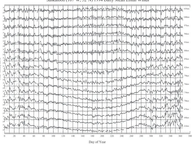
Saskatoon (107°W, 52°N) 1994 Daily Mean Zonal Winds
Day of Year 20 0 -20 61km 20 0 -20 64km 20 0 -20 67km 20 0 -20 70km 20 0 -20 73km 20 0 -20 76km 20 0 -20 79km 20 0 -20 82km 20 0 -20 85km 20 0 -20 88km 20 0 -20 91km 20 0 -20 94km 20 0 -20 97km 20 0 -20 100km 20 0 -20 103km Wind Velocity (m/s)
Fig. 1. The daily-mean winds for the zonal component at 61–103 km with 3 km intervals observed by the Saskatoon MF radar in 1994. The dotted curves are the band-pass filtered winds at period of 16 days (the values are doubled for prominence).
band of 11–24 days (i.e. less than 1% of the energy of those oscillations outside this band can pass through the filter).
Figure 1 shows Saskatoon daily-mean winds for the zonal component observed at 61–103 km with 3 km intervals in 1994, with the dotted curves representing the filtered winds of the 16-day wave (the values are doubled here for promi-nence). There are regular variations of the mean or back-ground winds. Below 82 km, an annual variation is dominant with winds varying from eastward to westward and then re-versing at about day 100 and day 260, respectively. Above 85 km, the semiannual variation is obvious, with westward winds appearing in the equinox seasons. But we are most concerned in this paper with those wave-like fluctuations that superimpose upon the mean winds. Generally, the fluctua-tions are strong when the mean winds are eastward, but be-come relatively quiet in the westward flows. In terms of the 16-day wave, the filtered winds also show the same features. Although the filtered waves seem reasonable and compara-ble to features in their “raw” winds, one still must ask the question as to whether these are real oscillations rather than responses of the filter to noise in the winds; in other words, ‘What are the confidence levels of the filter’s outputs?’.
3.2 Confidence of the filtered oscillations
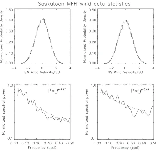
Although by theory of statistics the hypothesis testing can be done when the distribution of the data is known, in our situation it is very difficult to give analytically a statistical distribution of data output from such a filter even though the distribution of data input is known. However, a numerical test based on the Monte Carlo simulation can be used to re-alize this purpose. The idea is simply to construct numer-ous random (pure noise) sequences with the same statisti-cal characteristics as the real data, let them pass through the band-pass filter, and then obtain numerically the distribution of the outputs. Now first, ‘What are the statistical features of our radar data in both time and frequency domains?’. We normalized the winds, such as those shown in Fig. 1, by re-moving the mean values and then scaling by their standard deviations (SD), i.e. obtaining a zero mean and unit SD se-quence. The mean values and SDs are calculated with data in a moving window of 48 days. At the same time the Fourier transform is also made for each of these windowed data (af-ter detrending and tapering), and finally, all the spectra are averaged. In Fig. 2, the histograms show the distribution of normalized zonal (EW) and meridional (NS) winds of 1994
Fig. 2. Upper diagrams: The normalized (by standard deviation) distributions for the zonal (EW) and meridional (NS) winds at Saskatoon in 1994 (histograms), and the Gaussian (standard) distributions (dotted curves). Bottom diagrams: The averaged Fourier spectra for the above two components of wind; the dotted curves are their least-square fittings by an exponential function of frequency (f ) whose parameters are shown on the upper-right corner.
at Saskatoon. They are coincident with the Gaussian (stan-dard) distribution denoted by the dotted curves. Given that the winds are driven not by a single force but by a mixture of many dynamic sources, this is expected by the Central Limit Theorem which states that a sum of random variables, no matter in what different distributions they originally are, will become Gaussian distributed as more and more random variables are added together. The averaged spectra for the two components of winds are also displayed in Fig. 2. Even though they are averaged results, the peaks around 2, 5–7, 10, and 16 days (i.e. 0.50, 0.15–0.20, 0.10 and 0.06 cpd) are clear, especially for the zonal component. The dotted lines are least-square fittings of the spectra by an exponen-tial function of frequency. If the signals are treated as pure noise, they can be described as red noise having higher power at lower frequency, with the power reduction following a law of exponential attenuation.
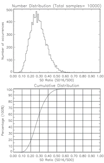
A great number of random sequences with Gaussian distri-butions and red noise characteristics have been used as input into our filter and a series of “16-day wave” outputs obtained. In Fig. 3, the SDs of 10 000 such outputs are calculated, and then a distribution of the occurring number against the ra-tio of the output and input SDs can be established, as shown
by the histogram. One can integrate the number distribution and change it into a cumulative distribution (P %) as shown in the bottom diagram of Fig. 3. In terms of statistics the cu-mulative distribution actually offers the percentage of chance (1−P %), of a ratio being larger than its corresponding value. In other words, when the filter output has an SD ratio larger than this value, there is (1 − P %) chance (significance) of the output oscillations being noise in the original input data, or P% chance (confidence) of there being real periodic oscil-lations. For example, when the SD ratio is larger than 0.40, we could be 90% sure that the output is a real signal instead of noise. The winds at other locations were also inspected and have similar statistical features, but only with minor dif-ferences on the spectral attenuation speed (the value of expo-nent).
3.3 The filtered 16-day waves
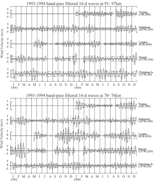
The 16-day filtered winds during 1993–1994 at five loca-tions, and two layers of 70–76 and 91–97 km in which the winds are altitudinally averaged before input into the fil-ter, are shown in Fig. 4. The envelope-like curves are the 95% confidence levels for the zonal 16-day waves (levels for
Fig. 3. The histogram is an occurrence (number) distribution of ra-tios of standard deviations of the output (SD16) and input signals (SD0) for a band-pass filter. The inputs are Gaussian random se-quences with red noise characteristics, and the outputs are the “16-day wave” series. The smooth curve is the cumulative distribution of the histogram. In terms of statistics the cumulative distribution actually offers the significance level 1 − P % (percentage of chance) of a ratio being larger than a certain value (level).
meridional ones not shown). It can be seen that most of the strong oscillations are well beyond the confidence levels. In general, the zonal component (solid curves) is greater in am-plitude than the meridional one (dashed curves), especially for those sites at mid- and lower latitudes, such as London, Hawaii and Christmas Island. However, at high-latitudes and in individual months, e.g. Saskatoon during November-December of 1993 at 70–76 km, and Tromsø during January– March of 1994 at 91–97 km, the meridional component is larger than or equivalent to the zonal one. The two com-ponents seem not generally in phase, but have some stable phase relationship when both exhibit strong oscillations. It is conspicuous that the 16-day waves are likely to demonstrate significant bursts (5∼7 m/s) during the late autumn through early spring months (October–April). Please note that the filtered amplitude may be suppressed by 30–40%, on
aver-age, due to the transition-band effect around the cut-off fre-quencies. In summer time, however, there are also relatively strong bursts, especially at the equatorial higher layer, such as in May–July of both 1993 and 1994. Their amplitudes are beyond the 95% confidence level as well. Another notice-able and interesting item is that the large bursts at the five sites often do not occur synchronously, even though some lo-cations are very close in terms of the large zonal wavelength (28 000 km) of the 16-day wave. For example, when there is a large burst of the wave at 70–76 km layer in October-November of 1994 at London, the wave activity at Saska-toon is relatively quiet. Instead, a strong wave appears after November of that year. Another example is in February– March of 1993 when the wave behaviour at Hawaii and Christmas Island is largely different. Such non-synchronized bursts had been noted earlier for London and Saskatoon, and were discussed in detail by Luo et al. (2002).
4 Wave amplitudes and periods 4.1 Spectral analysis method
The spectral estimation in this paper is based on the least-square fitting technique developed by Lomb (1976) and Scar-gle (1982). Using a time constant in the power-estimate equation, which makes it completely independent of any time shift, it weights the data on a “per point” basis instead of a “per time interval” basis. Therefore, this method can be es-pecially applied to unevenly time spaced data. Scargle’s def-inition of the time-translation invariance of the periodogram makes it exactly equivalent to a least-square fitting of a sine wave to data (Scargle, 1982). In addition, Scargle’s definition enables the periodogram to have a statistical exponential dis-tribution when the input signals are pure Gaussian noise. In this way it is possible to identify whether any large spectral peaks represent signal or noise; in other words, the Lomb-Scargle (L-S) periodogram can provide an estimate of the significance of each peak by examining the probability of its arising from a random fluctuation. This is probably why in recent years the L-S method was often applied in atmo-spheric data analysis. Based on the existing program routines Hocke (1998) has introduced a way to extend it for calcula-tion of phase spectra.
Before spectral analysis the missing data in the daily-mean winds are filled with linear interpolation when the length of the gap is small (less than 1/3 of the period of interest, i.e. 5 days). Otherwise, when it is longer than 5 days but less than 1/3 of the window length (a 48-day window used in this paper) for spectral analysis, they are replaced by Gaus-sian random values with the means and SDs matching the rest of the available data. The purpose for filling the gaps is to avoid the arbitrarily large false disturbance in the gap span when applying any spectral analysis based on harmonic fitting, such as the L-S method. This process was also de-scribed and used by the first author in an earlier paper (Luo
1993-1994 band-pass filtered 16-d waves at 91- 97km J F M A M J J A S O N D J F M A M J J A S O N D 1993 1994 5 0 -5 Tromso (19E,70N) 5 0 -5 Saskatoon (107W,52N) 5 0 -5 London (81W,43N) 5 0 -5 Hawaii (157W,21N) 5 0 -5 Christmas Is. (157W,2N) 5 0 -5 Tromso (19E,70N) 5 0 -5 Saskatoon (107W,52N) 5 0 -5 London (81W,43N) 5 0 -5 Hawaii (157W,21N) 5 0 -5 Christmas Is. (157W,2N)
1993-1994 band-pass filtered 16-d waves at 70- 76km
J F M A M J J A S O N D J F M A M J J A S O N D 1993 1994 5 0 -5 Tromso (19E,70N) 5 0 -5 Saskatoon (107W,52N) 5 0 -5 London (81W,43N) 5 0 -5 Hawaii (157W,21N) 5 0 -5 Christmas Is. (157W,2N) 5 0 -5 Tromso (19E,70N) 5 0 -5 Saskatoon (107W,52N) 5 0 -5 London (81W,43N) 5 0 -5 Hawaii (157W,21N) 5 0 -5 Christmas Is. (157W,2N) Wind Velocity (m/s) Wind Velocity (m/s)
Fig. 4. The filtered winds of 16-day waves at five locations during 1993–1994, and at two layers of 70–76 and 91–97 km. The filter is an FIR type with the kernel length of 64 days. The solid lines are for the zonal winds, and the dashed for the meridional winds. The envelope-like curves are the 95% confidence levels for the filtered wave in the zonal winds (levels for meridional ones not shown).
et al., 2001). However, if gaps are still longer than the above mentioned fit-length, no analysis will proceed.
We have used a running Hanning window with 48-day width to obtain “continuous” spectra. The 48-day is adopted since it is long enough to give significant parameters of the 16-day wave (with period resolution of ±3 days), yet short enough to give reasonable time sensitivity of the wave vari-ation (time resolution of about 13 days with Hanning win-dow). This is an empirically determined compromise be-tween time and frequency resolution.
4.2 The annual variability
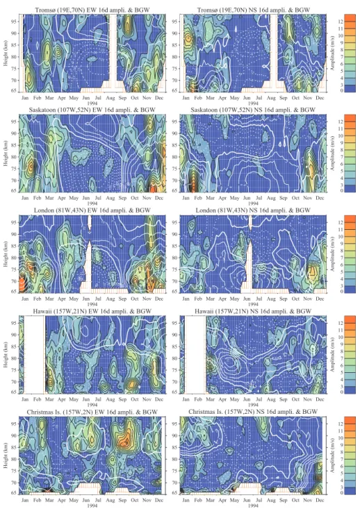
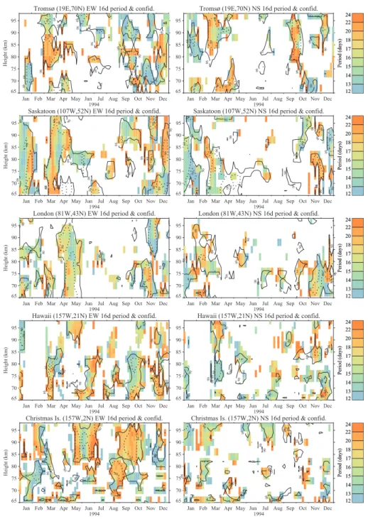
With the help of the above spectral method the wave parame-ters as a function of altitude and time can be derived. Figure 5 shows the 16-day wave amplitudes plus the mean winds, and Fig. 6 shows the period variability and confidence levels, of year 1994 at five locations. The wave amplitudes and
peri-ods come from the spectral integral values and spectral peak values within the band of 12–24 days.
We first take a look at Fig. 5 in which the zonal (EW) and meridional (NS) components of the wave and mean wind are displayed in the left and right columns, respectively. The mean wind contours step by 5 or 2 m/s for the EW or NS components, with solid lines denoting eastward/northward directions, dashed lines for the opposite directions, and thick ones for the zero wind lines. In general, the EW waves have larger amplitudes than the NS ones, and the waves have more regular annual variations at the three mid- and high-latitude locations (Tromsø, Saskatoon and London). Looking at these three locations the patterns for the mean zonal winds are very similar; the westward flows occur in summer-centred months below 85 km, with wind transitions in April and September. The difference is that at higher latitudes during the spring transition the westward flows are more likely to reach up into
0 3 4 5 6 7 8 9 10 11 12 Amplitude (m/s)
Tromsø (19E,70N) EW 16d ampli. & BGW
Jan Feb Mar Apr May Jun Jul Aug Sep Oct Nov Dec 1994 65 70 75 80 85 90 95 Height (km) 5 510 2015 5 5 5 10 5 5 -5 -25 -5 -5 -10 -15-5 -10 -15 -25 -25 -5 -20-15 -5 -5
Tromsø (19E,70N) NS 16d ampli. & BGW
Jan Feb Mar Apr May Jun Jul Aug Sep Oct Nov Dec 1994 65 70 75 80 85 90 95 8 6 12108 642 6 4 2 2 2 2 2 4 2 2 2 2 2 -4 -2 -2 -2 -2 -4 -2 -2 -2-4 -6 -8 -2 -2 -4 -2 -2 -4 -2 -2 -4 -4 -6 -4 -2 -2 -4 -8 -8 0 3 4 5 6 7 8 9 10 11 12 Amplitude (m/s)
Saskatoon (107W,52N) EW 16d ampli. & BGW
Jan Feb Mar Apr May Jun Jul Aug Sep Oct Nov Dec 1994 65 70 75 80 85 90 95 Height (km) 25 155 1020 25 30 5 5 10 15 20 25 30 5 10 15 5 5 5 5 -15 -10-5 -5 -25 -20 -30 -35 -40
Saskatoon (107W,52N) NS 16d ampli. & BGW
Jan Feb Mar Apr May Jun Jul Aug Sep Oct Nov Dec 1994 65 70 75 80 85 90 95 2 4 6 2 2 4 6 2 4 2 8 4 2 4 2 2 -2 -10 -8 -6 -4 -2 -2 -2 -4 -6 -2 -2-4 -4 -2 -2 -4 -6 0 3 4 5 6 7 8 9 10 11 12 Amplitude (m/s)
London (81W,43N) EW 16d ampli. & BGW
Jan Feb Mar Apr May Jun Jul Aug Sep Oct Nov Dec 1994 65 70 75 80 85 90 95 Height (km) 5 10 15 20 25 30 35 40 20 25 30 5 10 15 30 35 45 10 5 10 5 5 10 5 10 5 -10 -40 -35 -30 -25 -20 -15 -10 -5 -5 -5 -5 -25 -30-35 -25-30 -5 -10 -20 -10
London (81W,43N) NS 16d ampli. & BGW
Jan Feb Mar Apr May Jun Jul Aug Sep Oct Nov Dec 1994 65 70 75 80 85 90 95 2 4 2 2 4 6 2 6 8 10 12 1086 8 64 2 4 2 2 4 4 2 2 -4 -2 -2 -2 -4 -2 -4-6 -2 -8 -2 -2 -2 -8 -2 -2 -2 -4 0 3 4 5 6 7 8 9 10 11 12 Amplitude (m/s)
Hawaii (157W,21N) EW 16d ampli. & BGW
Jan Feb Mar Apr May Jun Jul Aug Sep Oct Nov Dec 1994 65 70 75 80 85 90 95 Height (km) 15 10 5 5 10 5 5 20 15 5 10 15 5 5 5 -5 -5 -5 -10 -10 -15 -20 -5 -25 -5 -5 -5
Hawaii (157W,21N) NS 16d ampli. & BGW
Jan Feb Mar Apr May Jun Jul Aug Sep Oct Nov Dec 1994 65 70 75 80 85 90 956 2 2 4 2 2 2 68 2 10 2 2 2 4 6 6 2 2 6 4 2 4 4 2 2 4 2 -2 -6 -8 -4 -2 -4 -6 -2 -6 -2 -4 -2 -4 -8 -6 -8 -2 -2 -2 -4 -2 -4 -2 -4 -6 -6 -2-4 -6 -6 -8 -4 0 3 4 5 6 7 8 9 10 11 12 Amplitude (m/s)
Christmas Is. (157W,2N) EW 16d ampli. & BGW
Jan Feb Mar Apr May Jun Jul Aug Sep Oct Nov Dec 1994 65 70 75 80 85 90 95 Height (km) 5 5 5 5 5 5 -5 -5 -5 -10 -10 -5 -5 -15 -5 -10 -5 -20 -15 -5 -5 -5 -5 -5 -5 -5 -5 -10 -5 -5
Christmas Is. (157W,2N) NS 16d ampli. & BGW
Jan Feb Mar Apr May Jun Jul Aug Sep Oct Nov Dec 1994 65 70 75 80 85 90 95 6 2 2 4 64 4 8 1012 2 2 2 2 2 8 22 4 2 42 2 -4 -2 -4 -6-2 -2 -8 -4 -6 -2 -2 -2 -4 -2 -4
Fig. 5. The 16-day wave amplitudes plus the background winds in a height-time section of year 1994 at five radar locations. The zonal (EW) and meridional (NS) components of the wave and the mean winds (line contours) are displayed in the left and right columns, respectively. The mean wind contours step by 5 or 2 m/s for the EW or NS winds, with solid lines denoting the eastward/northward directions, dashed lines the opposite directions, and thick ones the zero wind lines.
higher altitudes near 100 km. For the 16-day waves at these three locations, for either EW or NS components, they occur mostly in late autumn, winter and early spring and thus are coincident with the eastward mean zonal flows. During these seasons, the wave exists over a large part of the MLT region, with amplitudes generally decreasing with heights. Partic-ularly, at Tromsø and Saskatoon, the waves can be seen up to the lower thermosphere (100 km), while at London, they reach to about the mesopause layer (85 km) for most
situa-tions. Although theoretically it is already well established that the 16-day wave preferentially propagates in an east-ward background flow, observational evidences, such as in Fig. 5, support the prediction favourably and convincingly. Note, however, that the eastward flow regions are not solidly filled with 16-day PW activity, and also that in the weak westward flows, e.g. spring at Saskatoon and London, PW activity does occur. These indicate that the real atmosphere is more complex than any theoretical model. In the
sum-12 13 14 15 16 17 18 20 22 24 Period (days)
Tromsø (19E,70N) EW 16d period & confid.
Jan Feb Mar Apr May Jun Jul Aug Sep Oct Nov Dec 1994 65 70 75 80 85 90 95 Height (km) 99 99 99 99 99 99 99 99 99 99 99 90 90 90 90 90 90 90 90 90 90 90 90 90 90 90 90 90 90 90 90 90 90 90 90 12 13 14 15 16 17 18 20 22 24 Period (days)
Tromsø (19E,70N) NS 16d period & confid.
Jan Feb Mar Apr May Jun Jul Aug Sep Oct Nov Dec 1994 65 70 75 80 85 90 95 99 99 99 99 99 99 90 90 90 90 90 90 90 90 90 90 90 90 90 90 90 90 90 12 13 14 15 16 17 18 20 22 24 Period (days)
Saskatoon (107W,52N) EW 16d period & confid.
Jan Feb Mar Apr May Jun Jul Aug Sep Oct Nov Dec 1994 65 70 75 80 85 90 95 Height (km) 99 99 99 99 99 99 99 99 99 99 99 99 90 90 90 90 90 90 90 90 90 90 90 90 90 90 90 90 90 90 12 13 14 15 16 17 18 20 22 24 Period (days)
Saskatoon (107W,52N) NS 16d period & confid.
Jan Feb Mar Apr May Jun Jul Aug Sep Oct Nov Dec 1994 65 70 75 80 85 90 95 99 99 99 99 99 99 99 99 90 90 90 90 90 90 90 90 90 90 90 90 90 90 90 90 90 90 90 12 13 14 15 16 17 18 20 22 24 Period (days)
London (81W,43N) EW 16d period & confid.
Jan Feb Mar Apr May Jun Jul Aug Sep Oct Nov Dec 1994 65 70 75 80 85 90 95 Height (km) 99 99 99 99 99 99 99 90 90 90 90 90 90 90 90 90 90 90 90 90 90 90 12 13 14 15 16 17 18 20 22 24 Period (days)
London (81W,43N) NS 16d period & confid.
Jan Feb Mar Apr May Jun Jul Aug Sep Oct Nov Dec 1994 65 70 75 80 85 90 95 99 99 90 90 90 90 90 90 90 90 90 90 90 90 90 90 90 90 90 12 13 14 15 16 17 18 20 22 24 Period (days)
Hawaii (157W,21N) EW 16d period & confid.
Jan Feb Mar Apr May Jun Jul Aug Sep Oct Nov Dec 1994 65 70 75 80 85 90 95 Height (km) 99 99 99 99 99 99 99 99 90 90 90 90 90 90 90 90 90 90 90 90 90 90 90 12 13 14 15 16 17 18 20 22 24 Period (days)
Hawaii (157W,21N) NS 16d period & confid.
Jan Feb Mar Apr May Jun Jul Aug Sep Oct Nov Dec 1994 65 70 75 80 85 90 95 99 99 99 90 90 90 90 90 90 90 90 90 90 90 90 90 90 90 90 90 12 13 14 15 16 17 18 20 22 24 Period (days)
Christmas Is. (157W,2N) EW 16d period & confid.
Jan Feb Mar Apr May Jun Jul Aug Sep Oct Nov Dec 1994 65 70 75 80 85 90 95 Height (km) 99 99 99 99 99 99 99 99 99 99 90 90 90 90 90 90 90 90 90 90 90 90 90 90 90 90 90 90 12 13 14 15 16 17 18 20 22 24 Period (days)
Christmas Is. (157W,2N) NS 16d period & confid.
Jan Feb Mar Apr May Jun Jul Aug Sep Oct Nov Dec 1994 65 70 75 80 85 90 95 99 99 99 99 90 90 90 90 90 90 90 90 90 90 9090 9090 90 90 90 90 90 90 90 90 90 90 90
Fig. 6. Same as Fig. 5 but for the 16-day wave periods (colour bars) and the confidence levels (line contours) corresponding to the wave amplitudes shown in Fig. 5. Two confidence levels are drawn with dashed lines (99%) and solid lines (90%).
mer (May–August) westward flow, however, there is also a weak 16-day wave, especially for the EW component, at mid-latitudes. This is only seen over a limited range of altitudes. For example, at Saskatoon, it is around 80 km with ampli-tude of ∼5 m/s; at London, it can go down as low as 70 km in the westward flow with amplitude of ∼7 m/s. As we go to the subtropical and equatorial locations (Hawaii and Christ-mas Island), the waves are no longer winter dominated; in-stead, they spread to almost all seasons and altitudes of the MLT region. The best example is that at about 85–95 km at Christmas Island, strong wave activity appears all year round
(except for April), with peak amplitudes in May–June and September–October where the zonal winds are eastward and westward, respectively.
The particular background wind patterns may be related to the detailed latitudinal, altitudinal and seasonal distribu-tion of the 16-day waves. For example, the winter wave at Saskatoon can propagate up to the lower thermosphere prob-ably because the eastward flow there goes up to that region, but at London above ∼95 km, the westward flow is domi-nant. It should also be noted that the peak amplitude of the winter wave usually occurs at the maximum eastward flow,
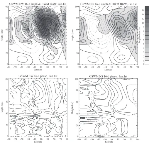
GSWM EW 16-d ampli & HWM BGW, Jan.1st -90 -70 -50 -30 -10 10 30 50 70 90 Latitude 0 20 40 60 80 100 Height (km) 10 10 10 20 20 30 40 50 10 20 -10 -20 -30 -40 -50 0 1 2 3 4 5 6 7 8 9 10 12 14 16 Amplitude (m/s)
GSWM NS 16-d ampli & HWM BGW, Jan.1st
-90 -70 -50 -30 -10 10 30 50 70 90 Latitude 0 20 40 60 80 100 Height (km) 10 10 10 20 20 30 40 50 10 20 -10 -20 -30 -40 -50 GSWM EW 16-d phase, Jan.1st -90 -70 -50 -30 -10 10 30 50 70 90 Latitude 0 20 40 60 80 100 Height (km) 90 135 45 45 45 90 135 135 45 90 45 45 90 90 135 45 90 135 45 90 -90 -45 -90 -90 -135 -45 -90 -90 -45 180 180 GSWM NS 16-d phase, Jan.1st -90 -70 -50 -30 -10 10 30 50 70 90 Latitude 0 20 40 60 80 100 Height (km) 45 90 45 90 135 45 90 135 90 135 90135 90 45 9045 90 90 45 45 45 45 90 135 -135 -45 -135 -90 -90 -135 -90 -45 -45 180
Fig. 7. The amplitudes and phases of the zonal and meridional wind 16-day perturbation from pole to pole obtained by the GSWM. Superimposed upon the amplitude grey contours are zonal background winds from the HWM93 with solid lines being the eastward. The model runs were under atmospheric conditions of 1 January. The unit of the wave amplitude and background wind is m/s. The phases are
the wave amplitude crests in longitude degree and step by 45◦.
e.g. the January/February peak at Saskatoon 75 km and Jan-uary peak at London 70 km. In other words, above this level there begins to be a negative wind shear in the zonal flow and probably in this region dynamical processes affect the upward propagating wave, such as reflection or dissipation. For example, in the GSWM model which was used by Luo et al. (2000) for the Saskatoon wave, dissipation due to eddy diffusion and gravity wave drag was shown to be significant. In summer, the wave can penetrate into the westward flow, e.g. at Saskatoon and London to the −25 m/s zonal mean wind lines ( ¯u). According to the simple analytical prop-agation condition 0 < ¯u − cx < Uc, by Charney and
Drazin (1961) (Ucis a critical calculated number, which
lim-its the strength of eastward winter flows into which PW can successfully propagate), and considering cx ≈ 20 m/s for
the westward propagating 16-day wave at mid-latitudes, the wave could only penetrate into somewhat lower-speed west-ward flows of up to −20 m/s. Planetary waves with larger phase speeds (e.g. the 5-day wave) could penetrate deeper into a given westward flow. In the real atmosphere, and in complex models such as the GSWM, weak penetration of the 16-day wave further into the westward flow is to be expected. At the lower latitudes the value of cxis larger than at higher
latitudes due to the larger latitude circle, if the wave number and period do not change, and this may explain why at Lon-don, Hawaii and Christmas Island there is more wave activity deeper into the westward flow in summer than at Tromsø or Saskatoon. On the other hand, at low-latitudes, the westward flows themselves are usually weaker (magnitudes less than 25 m/s) and would further facilitate the entering of the wave deeper into westward flows. Also, for an equatorial location like Christmas Island, waves from the Southern Hemispheric winter will have opportunities for propagation, e.g. during May–October.
The 16-day wave has been shown by numerical simula-tion to have a broad band of periods. The simulated response spectra for this wave indicate major peaks at 13.2 and 16.4 days under equinox atmospheric conditions, and at 15.7 days during solstice; allowing for other uncertainties and atmo-spheric variabilities, it should be in the range of 11.1–20.0 days (Salby, 1981b). As a complement and comparison of Fig. 5 the 16-day wave periods and confidence levels are cor-respondingly shown in Fig. 6. Two contour levels of con-fidence are plotted by dashed lines (99%) and solid lines (90%). It can be seen that the 90% levels are well coinci-dent with the areas with amplitude of about 4 m/s in Fig. 5;
in other words, the waves with amplitudes larger than 4 m/s should be, in principle, beyond the noise level. In the same way most of the periods displayed in the plots are also with this confidence. For those wave events that are “incessant” in a large altitude range, it seems that the periods are longer at lower heights and transit to shorter ones with increasing al-titude. For example, in March of Saskatoon, the zonal wave periods begin with ∼20–22 days at 65 km, and then decrease gradually with altitude; and in the April-May epoch at Lon-don, the zonal wave periods are generally a little longer at low altitudes. Another example is that at Hawaii there are several strips in March, June and September/October, respec-tively, also showing period-variations with height. On the other hand, the periods change with time as well, and some-times they are very conspicuous, even in a short time of span, for example, in January/February at Saskatoon.
When the wave variations associated with the EW and NS components are considered, the first thing that should be noted is that the amplitude variations at the same altitude for the two components are not always in proportion. For ex-ample, strong EW wave-activity well above the noise level (∼4 m/s) in March at Saskatoon appears at all altitudes, but there is almost no response or very weak response for the NS winds during the same time; vice versa, the NS winds show strong wave activity below 75 km in the first half of February, but it seems there is a valley for the EW winds at the same time. On the other hand, when there are relatively strong amplitudes for both components, their periods do not coincide exactly for most of the time, though sometimes they are fairly close. There is no general explanation available for this now. But since the Hough modes for the two compo-nents show different node positions, i.e. maximum ampli-tude around 40◦N for the zonal but minimum around 35◦N
for the meridional (Longuet-Higgins, 1968), changing atmo-spheric conditions (winds, temperatures) over several cycles of oscillation can likely lead to unique phase changes of each component. This is because the phase near the latitude with a minimum for the mode will change strongly as the node for the real atmosphere (likely distorted from the classical Hough mode structure) undergoes small shifts in position. This could lead to changes in the apparent period which we observe.
It is not easy to explain these variations of period with al-titude, month and location. Detailed comparisons with the GCMs, such as CMAM (Beagley et al., 1997) or TIME-GCM (Roble et al., 1994) for the MLT, where the latitudinal, longitudinal and modal structures for each component may be assessed and compared with observations, would be most valuable. This would help to isolate the factors responsible for change. At this point we note that simple comparisons of the observed period with the height variations of the back-ground flow do not follow any simple relationship. If the flow is nonstationary, e.g. due to quasi-stationary planetary waves or other long period waves or oscillations, then changes in observed period with time and height may be expected, as is the case for gravity waves (Manson et al., 1979; Zhong et al., 1996). However, it is clear from Fig. 6 that the observed
pe-riod in a given month of relatively stable background condi-tions, e.g. March at Saskatoon, decreases with height, while the mean flow is almost constant with height. It is appro-priate to argue that the real atmosphere does not behave in a simple fashion with regard to changes in an observed pe-riod with height and location. While there is a global re-sponse to the 16-day wave, there are significant observed dif-ferences between locations. We hypothesize that local con-ditions (winds, other PW modes, planetary wave and gravity wave interactions, and temperatures) may provide superpo-sition or favour responses or resonances at different periods at different sites. Also, changes in the latitudinal structure of the PW (mode adjustments), as well as changes in ver-tical wavelength with time, would lead to phase changes in the local oscillations which would appear as changes in the observed periods (Alex Pogoreltsev, 2001, private commu-nication). As we noted at the beginning of this paragraph, the best approach to understanding this is to carry out careful diagnostic experiments with sophisticated GCMs.
5 Comparisons with numerical model and satellite ob-servations
5.1 The GSWM 16-day waves
The Global Scale Wave Model (GSWM) is a two-dimensional, linearized, steady-state numerical model of global scale atmospheric waves based upon the early tidal model of Forbes (1982a, b). In recent years it has been ex-tended for the planetary wave studies, e.g. the 2-day wave (Hagan et al., 1993), the 16-day wave (Forbes et al., 1995), and the 6.5-day wave (Meyer et al., 1997). Briefly, it as-sumes that the atmosphere is a shallow, compressible, hydro-static and perfect gas; the model also includes full dissipative effects, i.e. ion drag, radiative cooling, surface friction and the molecular eddy diffusion of heat and momentum. After specifying the period, wave number and background wind, the perturbations upon a mean zonal background state can be solved subject to specified forcing. In the 16-day wave runs of this model, the inputs are westward propagating zonal wave number 1 with a period equal to 16 days. In the early work of Forbes et al. (1995), it had been shown that the re-sponse of the model is weakly dependent on the period vary-ing in the range of 12–20 days; namely, the assumption of a 14- or 16- or 19-day periodicity would result in only minor modification of the results. The forcing is on the uniform vertical velocity at the lower boundary, i.e. constant with latitude (forcing by specifying the vertical velocity with lat-itudinal dependence given by the Hough function was also run, but no big difference was found in the atmospheric re-sponse). The background winds utilize the HWM93 (Hedin et al., 1993) and the zonal mean temperatures are taken from the MSISE90 (Hedin, 1991). The model extends continu-ously from the surface to the ionosphere (∼1.5 km height grid) and from pole to pole (3◦ latitudinal grid) for all sea-sons.
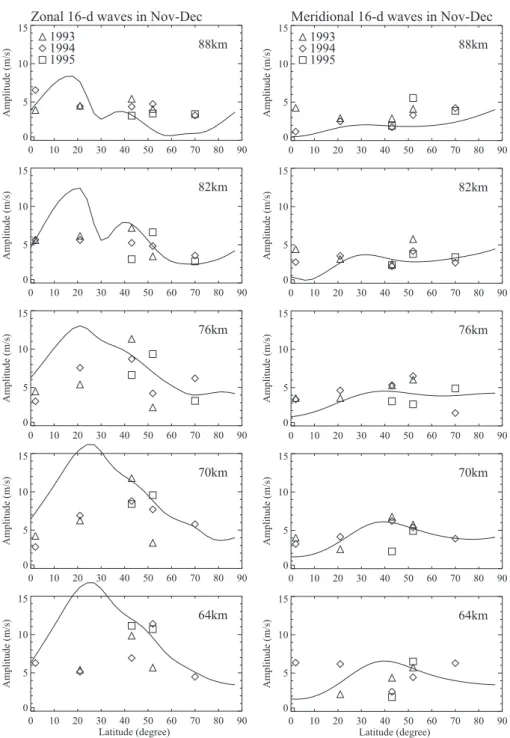
0 10 20 30 40 50 60 70 80 90 Latitude (degree) 0 5 10 15 Amplitude (m/s) 64km 0 10 20 30 40 50 60 70 80 90 0 5 10 15 Amplitude (m/s) 70km 0 10 20 30 40 50 60 70 80 90 0 5 10 15 Amplitude (m/s) 76km 0 10 20 30 40 50 60 70 80 90 0 5 10 15 Amplitude (m/s) 82km 0 10 20 30 40 50 60 70 80 90 0 5 10 15 Amplitude (m/s) 88km 1993 1994 1995
Zonal 16-d waves in Nov-Dec
0 10 20 30 40 50 60 70 80 90 Latitude (degree) 0 5 10 15 Amplitude (m/s) 64km 0 10 20 30 40 50 60 70 80 90 0 5 10 15 Amplitude (m/s) 70km 0 10 20 30 40 50 60 70 80 90 0 5 10 15 Amplitude (m/s) 76km 0 10 20 30 40 50 60 70 80 90 0 5 10 15 Amplitude (m/s) 82km 0 10 20 30 40 50 60 70 80 90 0 5 10 15 Amplitude (m/s) 88km 1993 1994 1995
Meridional 16-d waves in Nov-Dec
Fig. 8. The latitudinal variations of the 16-day wave amplitudes from radar observations and the GSWM. The scattering points are spec-tral amplitudes using available data of November/December of years 1993, 1994 and 1995 (denoted by triangles, diamonds and squares, respectively) at five radar locations and selected altitudes. The continuous lines are wave amplitudes from the model.
The early 16-day wave study has compared the annual cli-matologies at Saskatoon and from the GSWM at a corre-sponding latitude (Luo et al., 2000). Briefly, the excited 16-day PWs followed the zero zonal wind lines rather closely for their reductions and growths in the spring and autumn. In this paper, multiple radar observations will be compared with the model, focussing on the latitudinal variation. In view of the wave being most evident in the Northern Hemispheric win-ter, the modelling results under the conditions of 1 January are considered. In Fig. 7, the global amplitudes and phases of
the zonal and meridional wind 16-day perturbations from the GSWM are illustrated, and superimposed upon the amplitude contours are zonal background winds from the HWM93. As expected, the waves have strong amplitudes, as well as large extent in the Northern Hemisphere, where the eastward back-ground wind is prevailing, and are centred at 60–70 km and 20◦N for the EW, and 40◦N for the NS winds (note that this does not follow the classical Hough mode structures). How-ever, there are also substantial waves in the Southern Hemi-sphere, indicating some leakage over the equator and into
the summer upper mesosphere. The phase values represent the wave crest positions in degrees longitude in the context of only one wave cycle along the Earth’s latitudinal circle (zonal wave number 1). In the Northern Hemisphere, they suggest a very long vertical wavelength due to approximately con-stant phase with altitude when the amplitude is large; also, the phase values decrease toward higher latitudes. They are consistent with an equatorward phase propagation, as well as the westward propagation. In the summer hemisphere, the phase variations are not prominent; they roughly have a close phase when the amplitude is large.
5.2 Comparison on latitudinal variations and vertical struc-tures
Using the available data in November/December from sev-eral years (1993–1995), the spectral amplitudes of the 16-day wave at each radar location and selected altitudes are dis-played by the scattering points in Fig. 8; also shown are the continuous amplitude variations against latitude output from the model. Although there are only five radar sites here, they are well separated from the equator to the arctic in order to give a coarse latitudinal distribution for the wave amplitudes, which is desirable to be compared with the modelling results. The symbols of a triangle, diamond and square represent the amplitudes in 1993, 1994 and 1995, respectively. Although there are certain year-by-year differences below 82 km at the two mid-latitude locations, the general amplitude levels or latitudinal trends may not be impaired. First of all, both ob-served and modelling amplitudes show that they are usually larger at lower altitudes, and the zonal wave components are greater than the meridional ones, on average. For the zonal components below 76 km, the largest values appear at the latitude of London (43◦N); above 82 km, this mid-latitude maximum recedes and the amplitudes are consistently larger at lower latitudes, with a gradual decrease toward the arc-tic latitude. In a similar way but at somewhat different lat-itudes, the model amplitudes show peak values around 20-30◦N below 76 km, and with an altitude increase, the main peak moves to the lower latitude, which is, in principle, con-sistent with the radar amplitudes. For the meridional ampli-tudes, the radar points do not show any prominent peak with latitude change; instead, a weak increase with latitude may be displayed. Similarly, again, the model also shows an in-crease with latitude, except for a weak peak around 40◦N
be-low 70 km. Given that the observed amplitudes are only from several particular events, the above agreements are somewhat encouraging.
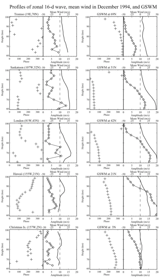
Though the altitude variations of the observed wave have been checked to some degree in the last couple of figures, it is still useful to show the height profiles of the amplitude and especially of the phase, and to compare them with modelling results. Figure 9 shows the profiles (60–100 km) for the zonal 16-day wave in the winter of 1994 at five locations, and the corresponding results from the model. For comparison, a 48-day data set centered at the 1 December is used to coordi-nate the model conditions; the observed wave amplitudes and
phases are obtained from the spectral analysis. Based upon the previous calculation of confidence levels (e.g. Figs. 4–6), amplitudes greater than 3 m/s here are considered significant, as well as their associated phases. This can also be confirmed by the consistency with the height of phases associated with amplitudes greater than 3 m/s. It should be noted that due to the longitudinal differences of the locations, the spectral phases are all calibrated to their zero-longitude according to an assumption of westward propagation with wave number 1, namely by subtracting their individual longitude. The pur-pose of doing this is to remove the longitudinal effect, but fo-cus rather on the latitudinal effect of the phases, and to make it easier to compare with the modelled ones. The phases are denoted by cross symbols and the amplitudes are denoted by connected diamonds; the mean wind profiles are also pro-vided by thick lines. In this winter month the mean winds of both the observation and the model almost all fall into a posi-tive area (eastward), with the best agreements at the arctic or equator latitudes. But at the mid- and low-latitudes, the radar winds show smaller speeds below 70∼80 km; given that the 24 h tides are stronger in this range of latitudes, this discrep-ancy is probably due to the tidal contamination of the radar winds, which has been referred to in Sect. 2. However, as we have said in that section, the PW amplitudes will be min-imally affected.
The model amplitude is maximum around 60–70 km, and then gradually decreases into insignificance at 90 km for the higher latitude locations, and transiting to 100 km for the lower ones. The radar winds also show large wave am-plitudes around 60–70 km, but the wave seems to be able to reach up to 100 km and beyond at higher latitude loca-tions. Meanwhile, on the amplitude profile itself, noticeable wave-like structures often exist, such as the Saskatoon file with three peaks at 64, 82 and 94 km, or the Hawaii pro-file with two peaks around 70 and 90 km. When checking their corresponding phase profiles, it can be found that the phases become approximately reverse across the amplitude troughs, i.e. with differences of nearly 180◦. This feature has been suggested as a vertical standing wave structure in a recent study (Luo et al., 2002) that is caused by the interfer-ence of the incident wave trains (upward) with the reflected waves (downward) in the MLT region, which forms several nodes/antinodes whose neighbouring phases are reversed.
For the model, the phase profiles are almost vertical in the plots at higher latitudes, but tilted a little more for the low-latitudes. This indicates that the vertical wavelength varies from very long to somewhat shorter, and the left tilted phase profile also implies downward phase propagation. Another point, which has been commented upon earlier in this sec-tion, is the equatorward phase propagation. This can be duced by their increasing phase values (longitudes in de-gree) from the arctic to equator. The radar wind phases, however, do not appear in such a simple fashion. The rea-sons, in addition to the observational noise, have to do with some phase uncertainty due to the wave period slightly vary-ing with height, as in Fig. 6. In addition, the interference of the incident and reflected waves will modify or alter the
Tromso (19E,70N) 0 100 200 300 Phase 60 70 80 90 100 Height (km) 0 5 10 15 20 Amplitude (m/s) 60 70 80 90 100 -50 -25Mean Wind (m/s)0 25 50 GSWM at 69N 0 100 200 300 Phase 60 70 80 90 100 Height (km) 0 5 10 15 20 Amplitude (m/s) 60 70 80 90 100 -50 -25Mean Wind (m/s)0 25 50 Saskatoon (107W,52N) 0 100 200 300 Phase 60 70 80 90 100 Height (km) 0 5 10 15 20 Amplitude (m/s) 60 70 80 90 100 -50 -25Mean Wind (m/s)0 25 50 GSWM at 51N 0 100 200 300 Phase 60 70 80 90 100 Height (km) 0 5 10 15 20 Amplitude (m/s) 60 70 80 90 100 -50 -25Mean Wind (m/s)0 25 50 London (81W,43N) 0 100 200 300 Phase 60 70 80 90 100 Height (km) 0 5 10 15 20 Amplitude (m/s) 60 70 80 90 100 -50 -25Mean Wind (m/s)0 25 50 GSWM at 42N 0 100 200 300 Phase 60 70 80 90 100 Height (km) 0 5 10 15 20 Amplitude (m/s) 60 70 80 90 100 -50 -25Mean Wind (m/s)0 25 50 Hawaii (155W,21N) 0 100 200 300 Phase 60 70 80 90 100 Height (km) 0 5 10 15 20 Amplitude (m/s) 60 70 80 90 100 -50 -25Mean Wind (m/s)0 25 50 GSWM at 21N 0 100 200 300 Phase 60 70 80 90 100 Height (km) 0 5 10 15 20 Amplitude (m/s) 60 70 80 90 100 -50 -25Mean Wind (m/s)0 25 50 Christmas Is. (157W,2N) 0 100 200 300 Phase 60 70 80 90 100 Height (km) 0 5 10 15 20 Amplitude (m/s) 60 70 80 90 100 -50 -25Mean Wind (m/s)0 25 50 GSWM at 3N 0 100 200 300 Phase 60 70 80 90 100 Height (km) 0 5 10 15 20 Amplitude (m/s) 60 70 80 90 100 -50 -25Mean Wind (m/s)0 25 50
Profiles of zonal 16-d wave, mean wind in December 1994, and GSWM
Fig. 9. The phase and amplitude profiles (60–100 km) for the zonal 16-day wave in the winter of 1994 at five locations, and the corresponding results from the GSWM. The spectral phases for winds at different locations are all calibrated to the zero-longitude according to westward propagation of zonal wave number 1. The phases are denoted by cross symbols and the amplitudes by connected diamonds. The mean wind profiles are also provided by thick lines.
phase manifestation, especially when wave attenuation ex-ists in practice, which results in the reflected waves possess-ing different amplitudes. But above ∼85 and until 100 km, the radar wind phases are relatively stable at all locations; if we only check the phases in this altitude range, they do indicate orderly and an almost linear increase from Tromsø of about 20◦, Saskatoon of 100◦, London of 140◦, Hawaii of 240◦, and to Christmas Island of 320◦. Furthermore, the model shows that the phase varies nearly by one cycle (360◦) across the hemisphere and so does the observed phase. This is also consistent with the wave amplitude configuration in Fig. 7, where the nodal positions are roughly at 70◦N and the equator. The Hough mode nodes are clearly modified by the complex processes in the model and the real atmosphere. 5.3 The HRDI 16-day waves
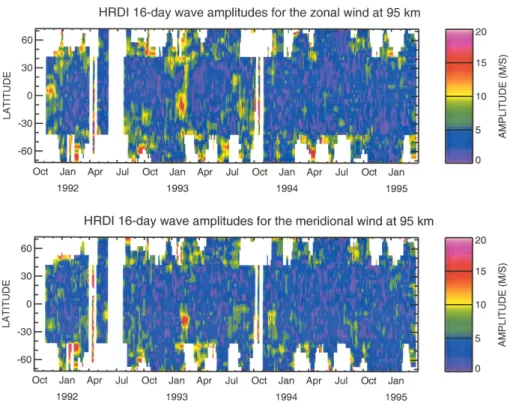
The High-Resolution Doppler Imager (HRDI) is an in-strument aboard the Upper Atmosphere Research Satellite (UARS). HRDI measures the horizontal winds by observ-ing the Doppler shift of the emission and absorption lines of molecular oxygen, mainly in daytime in small atmospheric volumes (4 km in height by 50 km in width) above the limb of the Earth. The height of 95 km is selected because around this altitude a narrow chemical source emission layer makes nighttime observations also available, and this provides a maximum coverage of local time to minimize the tidal ef-fects on the day-to-day database.
The 16-day wave amplitudes from the HRDI measure-ments during 1992–1995 at all available latitudes are shown in Fig. 10. This graph was produced by fitting a westward travelling 16-day wave of zonal wave number 1 along each latitude circle, while using a 32-day time window with fits every 4◦in latitude. It clearly indicates that the 16-day wave activity is a “winter” or “non-summer” phenomenon. The amplitudes are generally strong during October through De-cember to April, and weak during summertime for the North-ern Hemisphere; and weak during spring-summer (October– January) for the Southern Hemisphere. The strong wave ac-tivities mainly fall into the 40◦–60◦ latitude band of both hemispheres. However, there are many gaps at the higher latitudes and these make it difficult to make such general-izations in some months. In addition, the zonal wave am-plitudes are usually larger than the meridional ones. There are also some prominent wave activities around the equato-rial and tropical regions, but they appear without preferen-tial seasons. The general features mentioned above are in good agreement with those from the radar wind analyses, in not only the seasonal variations, but also the intermittence in time and space. However, some specific comparisons be-tween this graph and the upper portion of Fig. 4 or 5 are not always incontestable, especially at lower latitudes. For ex-ample, around the equator, the HRDI shows strong wave en-hancements in January/February and August/September of 1993 and is relative quiet through 1994 (up to 10 m/s in May–September); while the radar wind at Christmas Island, in spite of some small “bursts” during the above months
of 1993, also shows large wave activities in May 1993 and for almost all the seasons through 1994 (especially May– October). Considering that the HRDI 16-day waves come from a global fit, and that complex dynamical processes may happen locally (Sect. 4.2) for the wave propagation, e.g. the longitudinal differences of wave guide, the differences be-tween the HRDI and radar 16-day waves are understandable. Also, Kelvin waves in the mesosphere, which may include periods up to 13 days (Smith, 1999), may have added, to some degree, variance to the radar wind sequences and con-tours (Figs. 4 and 5) at Christmas Island. These waves would not have contributed to the HRDI plots (Fig. 10) due to the use of global westward wave fitting. It is worth noting that the HRDI 16-day wave, even globally, is also episodic in its occurrences, and generally occurs in quite narrow latitude bands for each event. This episodic nature was also seen in our radar contour plots (Fig. 5).
6 Discussions and conclusions
Charney and Drazin (1961) considered the vertical propaga-tion of a stapropaga-tionary planetary wave in an atmospheric medium of variable refractive index (ν). They argued that in regions where ν has a real value, the vertical propagation of planetary wave energy is freely permitted; an infinite layer in which
ν is imaginary will reflect wave totally. But if ν is imagi-nary in an intermediate layer, there will be partial reflection in this middle layer. Based upon their refractive index equa-tion, but with the characteristics of the propagating 16-day wave mode, and with more recent models for atmospheric temperature and density (i.e. MSISE90), and the zonal back-ground winds (HWM93), we have also calculated ν2 as a function of height for different seasons in this paper. Fig-ure 11 shows the situations for January and July at latitudes of 30◦, 45◦, and 60◦N, which are represented by thick solid, dotted, and thin solid lines, respectively. In winter, ν2 is mainly positive through the stratosphere to the mesosphere (20–70 km). The positive values exist until higher altitudes, especially at the lower latitudes; this is consistent with the GSWM, which shows less wave activities above 85 km at high latitudes (Fig. 9). It should be noted that at a certain layer of 60–80 km, the index-squared protrudes into the neg-ative region where the wave should be partially reflected. The reflected and incident wave may therefore interfere and form standing waves as in Fig. 9. In summer, however, negative
ν2appears in the whole upper stratosphere and mesosphere (30–80 km), which will totally block the wave propagation. Wave existence is permitted above 80 km, provided that the waves entering into the westward flow have propagated from other latitudes where full propagation is allowed. The cal-culations of ν2 appear to be a useful tool if the GSWM is unavailable for particular wave propagation conditions.
The theoretical and modelling preference, that the verti-cal propagation of the 16-day wave up to the MLT region is permitted through the eastward flows, is supported by the observations shown in this paper. First, the strongest wave
Fig. 10. The latitude-time amplitudes of the 16-day wave from HRDI wind measurements during 1992–1995. The amplitudes were produced
by fitting a 16-day wave of zonal wave number 1 along each latitude circle, while using a 32-day time window and fitting every 4◦in latitude.
The upper panel is for the zonal wind, and the bottom is for the meridional wind.
Fig. 11. The refractive index squares (ν2) for vertical propagation of the 16-day waves in January and July at latitudes of 30◦, 45◦, and
60◦N, which are represented by thick solid, dotted, and thin solid lines, respectively.
amplitudes, whether for zonal or meridional winds, are all associated with the eastward zonal background wind, i.e. the “winter” months. In the height-month contours (Fig. 5) for middle and high-latitude locations, there are clear boundaries near the zero-wind line in April and September (to be strict, it should be the −20 m/s wind line for a westward travelling 16-day wave), which separate the winter and summer wave activity. Second, the vertical standing wave structure in win-ter (Fig. 9) also corroborates the idea of an upward propa-gating wave. Additionally, the latitudinal phase variation of Fig. 9 implies an equatorward phase propagation that is also
in good agreement with the model.
The existence of summer wave activity is assumed to be by inter-hemispheric ducting of the 16-day wave, or by in situ generation through the 16-day modulation of upward propagating gravity waves and their dissipation in the sum-mer hemisphere (Smith, 1996). In this paper, the sumsum-mer wave occurs at different heights for different locations, even though some sites are geographically very close. This per-haps gives a hint of ducts connected to the other hemisphere across the equator, where different ducting paths may map to the different latitudes and longitudes. Furthermore, the lower