HAL Id: insu-02440391
https://hal-insu.archives-ouvertes.fr/insu-02440391
Submitted on 22 Jun 2020
HAL is a multi-disciplinary open access
archive for the deposit and dissemination of
sci-entific research documents, whether they are
pub-lished or not. The documents may come from
teaching and research institutions in France or
abroad, or from public or private research centers.
L’archive ouverte pluridisciplinaire HAL, est
destinée au dépôt et à la diffusion de documents
scientifiques de niveau recherche, publiés ou non,
émanant des établissements d’enseignement et de
recherche français ou étrangers, des laboratoires
publics ou privés.
Distributed under a Creative Commons Attribution - NoDerivatives| 4.0 International
consistency, merits and pitfalls
Matthias Sinnesael, David de Vleeschouwer, Christian Zeeden, Sietske J.
Batenburg, Anne-Christine da Silva, Niels de Winter, Jaume Dinarès-Turellh,
Anna Joy Drury, Gabriele Gambacorta, Frederik J. Hilgen, et al.
To cite this version:
Matthias Sinnesael, David de Vleeschouwer, Christian Zeeden, Sietske J. Batenburg, Anne-Christine
da Silva, et al.. The Cyclostratigraphy Intercomparison Project (CIP): consistency, merits and
pit-falls. Earth-Science Reviews, Elsevier, 2019, 199, pp.102965. �10.1016/j.earscirev.2019.102965�.
�insu-02440391�
Contents lists available atScienceDirect
Earth-Science Reviews
journal homepage:www.elsevier.com/locate/earscirev
Invited review
The Cyclostratigraphy Intercomparison Project (CIP): consistency, merits
and pitfalls
Matthias Sinnesael
a,b,*
, David De Vleeschouwer
c, Christian Zeeden
d,e, Sietske J. Batenburg
f,
Anne-Christine Da Silva
g, Niels J. de Winter
a, Jaume Dinarès-Turell
h, Anna Joy Drury
c,i,
Gabriele Gambacorta
j, Frederik J. Hilgen
k, Linda A. Hinnov
l, Alexander J.L. Hudson
m,
David B. Kemp
n, Margriet L. Lantink
k, Jiří Laurin
o, Mingsong Li
p, Diederik Liebrand
c, Chao Ma
q,
Stephen R. Meyers
r, Johannes Monkenbusch
s, Alessandro Montanari
t, Theresa Nohl
u,
Heiko Pälike
c, Damien Pas
v, Micha Ruhl
w, Nicolas Thibault
s, Maximilian Vahlenkamp
c,
Luis Valero
x, Sébastien Wouters
g, Huaichun Wu
y, Philippe Claeys
aaAnalytical, Environmental and Geo-Chemistry, Vrije Universiteit Brussel, Pleinlaan 2, B-1050, Brussels, Belgium bDepartment of Geology, Ghent University, Ghent, Belgium
cMARUM — Center for Marine Environmental Sciences, University of Bremen, Leobener Straße, 28359, Bremen, Germany
dIMCCE, Observatoire de Paris, PSL Research University, CNRS, Sorbonne Universités, UPMC Univ. Paris 06, Univ. Lille, 75014, Paris, France eLIAG – Leibniz Institute for Applied Geophysics, Geozentrum Hannover, Stilleweg 2, 30655, Hannover, Germany
fGéosciences Rennes, Université de Rennes 1, Campus de Beaulieu, 35042, Rennes, France
gPétrologie Sédimentaire, B20, Allée du Six Août, 12, Quartier Agora, Liège University, Sart Tilman, 4000, Liège, Belgium hIstituto Nazionale di Geofisica e Vulcanologia, Via di Vigna Murata 605, I-00143, Rome, Italy
iDepartment of Earth Sciences, University College London, Gower Street, London, WC1E 6BT, UK
jDipartimento di Scienze della Terra “A. Desio”, Università degli Studi di Milano, Via Mangiagalli 34, Milan, 20133, Italy kDepartment of Earth Sciences, Utrecht University, Princetonlaan 8a, 3584 CB, Utrecht, the Netherlands
lDepartment of Atmospheric, Oceanic, and Earth Sciences, George Mason University, Fairfax, VA, 22030, USA mCamborne School of Mines and Environment and Sustainability Institute, University of Exeter, Penryn, TR10 9FE, UK
nState Key Laboratory of Biogeology and Environmental Geology, School of Earth Sciences, China University of Geosciences, Wuhan, 430074, China oInstitute of Geophysics, Academy of Sciences of the Czech Republic, Boční II/1401, Praha 4, Czech Republic
pDepartment of Geosciences, Pennsylvania State University, University Park, PA, 16802, USA
qDepartment of Computer Science, University of Idaho, 875 Perimeter Drive MS 1010, Moscow, ID, 83844-1010, USA rDepartment of Geoscience, University of Wisconsin-Madison, Madison, WI, USA
sDepartment of Geosciences and Natural Resource Management, University of Copenhagen, Øster Voldgade 10, DK-1350, Copenhagen K, Denmark tOsservatorio Geologico di Coldigioco, Cda. Coldigioco 4, 62021, Apiro, Italy
uUniversität Erlangen-Nürnberg, GeoZentrum Nordbayern, Fachgruppe Paläoumwelt, Loewenichstrasse 28, D-91054, Erlangen, Germany vDepartment of Earth Sciences, Paleomagnetic Laboratory, Utrecht University, Fort Hoofddijk, the Netherlands
wGeology, School of Natural Sciences, Trinity College, Dublin, Ireland
xLaboratori de Paleomagnetisme CCiTUB-CSIC, Institut de Ciències de la Terra Jaume Almera, 08028, Barcelona, Spain ySchool of Ocean Sciences, China University of Geosciences, Beijing, 100083, China
A B S T R A C T
Cyclostratigraphy is an important tool for understanding astronomical climate forcing and reading geological time in sedimentary sequences, provided that an imprint of insolation variations caused by Earth’s orbital eccentricity, obliquity and/or precession is preserved (Milankovitch forcing). Numerous stratigraphic and paleoclimate studies have applied cyclostratigraphy, but the robustness of the methodology and its dependence on the investigator have not been systematically evaluated. We developed the Cyclostratigraphy Intercomparison Project (CIP) to assess the robustness of cyclostratigraphic methods using an experimental design of three artificial cyclostratigraphic case studies with known input parameters. Each case study is designed to address specific challenges that are relevant to cy-clostratigraphy. Case 1 represents an offshore research vessel environment, as only a drill-core photo and the approximate position of a late Miocene stage boundary are available for analysis. In Case 2, the Pleistocene proxy record displays clear nonlinear cyclical patterns and the interpretation is complicated by the presence of a hiatus. Case 3 represents a Late Devonian proxy record with a low signal-to-noise ratio with no specific theoretical astronomical solution available for this age. Each case was analyzed by a test group of 17-20 participants, with varying experience levels, methodological preferences and dedicated analysis time. During the CIP 2018 meeting in Brussels, Belgium, the ensuing analyses and discussion demonstrated that most participants did not arrive at a perfect solution, which may be partly explained by the limited amount of time spent on the exercises (∼4.5 hours per case). However, in all three cases, the median solution of all submitted analyses
https://doi.org/10.1016/j.earscirev.2019.102965
Received 25 June 2019; Received in revised form 20 September 2019; Accepted 22 September 2019
⁎Corresponding author.
E-mail address:[email protected](M. Sinnesael).
Available online 30 October 2019
0012-8252/ © 2019 The Authors. Published by Elsevier B.V. This is an open access article under the CC BY-NC-ND license (http://creativecommons.org/licenses/BY-NC-ND/4.0/).
accurately approached the correct result and several participants obtained the exact correct answers. Interestingly, systematically better performances were obtained for cases that represented the data type and stratigraphic age that were closest to the individual participants’ experience. This experiment demonstrates that cyclostratigraphy is a powerful tool for deciphering time in sedimentary successions and, importantly, that it is a trainable skill. Finally, we emphasize the importance of an integrated stratigraphic approach and provide flexible guidelines on what good practices in cyclostratigraphy should include. Our case studies provide valuable insight into current common practices in cyclostratigraphy, their potential merits and pitfalls. Our work does not provide a quantitative measure of reliability and uncertainty of cyclostratigraphy, but rather constitutes a starting point for further discussions on how to move the maturing field of cyclostratigraphy forward.
1. Introduction
Cyclostratigraphy is the branch of stratigraphy relating to the se-dimentary record of astronomically forced paleoclimate change and it includes applications to geologic correlation and the determination of geologic time (Fischer et al., 1988;Schwarzacher, 1993;Hilgen et al., 2004; Strasser et al., 2006; Hinnov and Hilgen, 2012). Cyclostrati-graphy, as typically practiced, is specifically concerned with the
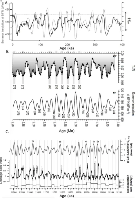
identification of “Milankovitch cycles” in the sedimentary record (Fig. 1), and the astronomical parameters that force these cycles as described inMilankovitch (1941)(Berger, 1978;Berger et al., 1993, 2010). An integral goal of cyclostratigraphy is a detailed understanding of astronomical climate forcing. Cyclostratigraphy commonly uses “proxies” for paleoclimatic change measured (e.g. sediment composi-tion, isotopic ratios and paleontological abundances) at suitably high resolution to capture cyclic climate variations through stratigraphic
Fig. 1. Examples of recorded astronomical climate forcing (“Milankovitch cycles”) in the sedimentary record: (A) Antarctic Vostok ice-core air δ18O record (Hay,
2013) based onPetit et al. (1999)andShackleton (2000). (B) Late Pliocene Eastern Mediterranean ODP Site 967 Ti/Al record (Lourens et al., 2001). (C) Late Miocene Monte dei Corvi outcrop (central Italy) lithological color index record (Zeeden et al., 2014).
successions.
“Astrochronology” pertains to the calibration of geologic time by the Earth’s astronomical parameters by means of cyclostratigraphy. “Tuning” involves the correlation and pattern-matching of cyclostrati-graphic interpretations to an astronomical solution, an astronomically forced climate model or specific astronomical terms (see definitions in Meyers, 2019). A more conservative use of the term “tuning” refers to the correlation and pattern-matching to astronomical solutions only. There are many potential tuning targets in cyclostratigraphy: an as-tronomical solution that consists of one or more asas-tronomical para-meters (Hays et al., 1976; Lourens et al. 1996; Hinnov, 2018a), in-solation curves (Köppen and Wegener, 1924; Milankovitch, 1941; Laskar et al. 2004), glacial models (Imbrie and Imbrie, 1980), and as-tronomically tuned stratigraphic reference datasets (Lisiecki and Raymo, 2005;De Vleeschouwer et al., 2017a).
If one chooses to tune to an astronomical solution, different con-straints apply depending on the solution. The Earth’s obliquity and precession solutions are not well constrained beyond 10 Ma, an issue that arises from the poor constraints on the long-term evolution of the Earth-Moon system due to the poorly known history of tidal dissipation and/or dynamical ellipticity (Laskar et al., 1993; Berger and Loutre, 1994;Pälike and Shackleton, 2000;Lourens et al., 2001;Laskar et al., 2004;Lourens et al., 2004;Zeeden et al., 2014;Waltham, 2015;Meyers and Malinverno 2018). The astronomical solution for planetary orbital dynamics (orbital eccentricity and inclination) is highly consistent for different numerical algorithms and initial conditions for the past ∼50 million years, but diverges quickly for times prior to that (Laskar et al., 2004,2011a,b;Zeebe, 2017). However, the orbital eccentricity solution can be extended into the early Mesozoic if only the 405-kyr (g2-g5) term
is considered (Kent et al., 2018). The gi’s and si’s represent the secular
frequencies of the planets (i, i=1 for Mercury etc.) in our Solar System and are related to the deformation and inclination of the respective planets’ orbital planes by gravitational forces (Laskar et al., 2004). The g2-g5term arises from the gravitational interaction between Venus and
Jupiter, and is extremely stable and often referred to as the “me-tronome” of the Solar System (Kent et al., 2018;Hinnov, 2018a). Un-fortunately, the Paleozoic and Precambrian are lacking a robust astro-nomical solution. Nonetheless, sedimentary records can still be tuned to astronomical terms of known periodicity, e.g. g2-g5orbital eccentricity
or orbital inclination s3-s6terms (Laskar et al., 2004; Boulila et al.,
2018;Hinnov, 2018b).
Other strategies approach the astronomical tuning problem differ-ently: joint constraints from two interrelated astronomical parameters, e.g., amplitude modulation of the precession index by the orbital ec-centricity (Meyers, 2015, 2019), or frequency ratio methods (e.g., average spectral misfit (Meyers and Sageman, 2007); evolutionary correlation coefficients (Li et al., 2018), or a combination of these (Meyers, 2015, 2019). Such approaches can provide enhanced con-fidence in the relative time scales developed from cyclostratigraphy,
i.e., “floating astrochronologies” (Hinnov, 2013; Meyers, 2019). The robustness of a floating astrochronology must be tested and a numerical age established through an integrated stratigraphic approach based on other independent methods of correlation (Table 1), ideally through high-precision radioisotopic geochronology, to yield an “anchored as-trochronology” (Hinnov, 2013;Meyers, 2019).
The modern rationale for developing an astrochronology based on a cyclostratigraphic analysis was established byHays et al. (1976). Over the years, increasingly innovative methodologies have been proposed to limit the subjective aspects of signal manipulation. Certain quantitative approaches remain debated, notably the issue of potential false nega-tives and false posinega-tives in statistical hypothesis testing of cyclostrati-graphic power spectra (Hilgen et al., 2015 and references therein; Kemp, 2016;Smith and Bailey, 2018;Hinnov et al., 2018;Crampton et al., 2018;Weedon et al., 2019). Consequently, methods that consider amplitude relationships in addition to spectral power are gaining in-creasing popularity in an effort to avoid subjectivity (e.g.Zeeden et al., 2015;Meyers, 2019, and references therein). Other unresolved issues affecting cyclostratigraphy include: (i) the completeness of strati-graphic records (i.e. defining and dealing with hiatuses; ensuring a complete composite section or “splice”); (ii) the pathway between as-tronomically forced climate, climate-forced sedimentation and the stratigraphic record; (iii) independent age control in cyclostratigraphy; (iv) uncertainties in the astronomical parameters of the deep-time geologic past; and (v) diagenetic origin or overprint of cycles in sedi-mentary successions. Despite recent insights and the development of new tools (e.g. reviews byHinnov, 2018a;Meyers, 2019) cyclostrati-graphy and astrochronology remain controversial to some extent, al-though they are becoming increasingly accepted as providing a reliable high-precision approach to time scale development and paleoclima-tology in deep time.
The robustness of the chosen methodology, independence of the investigator and reproducibility has never been systematically tested for cyclostratigraphy. The Cyclostratigraphy Intercomparison Project (CIP) was designed to address this issue, and to ask the following fun-damental questions: “What happens when a considerable number of independent researchers in the field of cyclostratigraphy investigate the same case study? How large are the differences between the answers? Where do the potential differences originate from? Can the cyclos-tratigraphic community reduce these discrepancies, and if so, how?”
The CIP was set up by the three first authors of this paper (core team), and the work was initiated by making contact with potentially interested scientists through a mailing list, a website (http://we.vub.ac.be/en/ cyclostratigraphy-intercomparison-project), a ResearchGate page (https:// www.researchgate.net/project/Cyclostratigraphy-Intercomparison-Project) and presentations at four recent international conferences (Sinnesael et al., 2017a,b,c,2018). The approach of the project was also inspired by the electrical engineering Nonlinear System Identification Benchmarks Work-shop series (http://www.nonlinearbenchmark.org, Schoukens and Noël,
Table 1
Geologic stratigraphic standardization is the key for defining a high-precision, globally correlated geologic time scale (Hedberg, 1976). Chronostratigraphy con-tributes fundamentally to the definition of geologic time and global correlation (Gradstein et al., 2012), and its main components comprise the criteria required for cyclostratigraphy and astrochronology. During any cyclostratigraphic analysis, the user should refer to an additional stratigraphic methodology to develop a useful astrochronology. The combination of multiple stratigraphic methodologies is referred to as an “Integrated Stratigraphic Approach”.
Methodology Notes
Biostratigraphy The paleontological record, classified into biozonal successions and assigned relative ages, provides a regional and sometimes globally applicable subdivision for the time succession of geological events.
Chemostratigraphy Isotope geochemistry of marine carbonate provides a continuous record of temperature (O), ice volume (O), carbon cycle perturbations (C), productivity (C) and continental runoff/submarine volcanism balance (Sr).
Event Stratigraphy Ice ages, oceanic anoxic events, hyperthermal events, large igneous provinces and extra-terrestrial impacts with global-scale influence provide additional global correlation tie-points.
Radioisotopic Geochronology Radioisotopic dating provides the defining information for numerical geologic time scales; principal techniques include U-Pb and40Ar/39Ar
geochronology.
Magnetostratigraphy The geologic sequence of geomagnetic field polarity reversals and past magnetic field intensities provides a globally significant set of time correlation points when calibrated with other chronostratigraphic evidence.
2017), which unites their respective community once a year to test and tackle specific state-of-the-art research questions. Based on these discus-sions, and initial feedback from the community, the CIP core team designed three artificial case studies. The decision to work with artificial case studies was motivated, besides practical considerations, by the key advantage of having the potential for validation of the submitted results, which cannot be guaranteed for real cases. The case studies were designed to provide minimalist stratigraphic information in order to not prescribe a particular approach to participants. The case studies do not per se represent typical cyclostratigraphic studies as present in the literature, as these often have more detailed stratigraphic constraints that assist the interpretation process. Hence, the cases represent “poorly constrained scenarios” in terms of boundary conditions and do not provide a conclusive reference for the re-liability of the field of cyclostratigraphy. CIP’s strength is that the use of artificial cases can test critical issues such as the effect of using different methodological approaches or hiatus detection. The aim of the CIP is to obtain insights into, test and compare common practices in cyclostrati-graphy. This CIP serves as a starting point for further discussions and pro-vides indications about the directions in which this field can progress.
2. Methods
2.1. Study design
Each CIP core team member designed one case study, and together they discussed and refined the three cases. Each case study was pre-sented as a data set with an accompanying text and figure with con-textual information (see Sections 2.2–2.4). Initially, the three case studies were independently tested by a small group of researchers (A.C. Da Silva, N.J. de Winter, C. Ma) to allow potential adaptation of the design following feedback. This feedback confirmed the validity of the first and third case studies, and led to modifications of the instruction text for the second case. Therefore, initial test results for Cases 1 and 3 were included in the final CIP compilation, but were omitted for Case 2. Subsequently, all three cases were made openly accessible online for about three months to all interested scientists. A total of 24 participants filled in a standardized form (to enable direct comparison), including:
level of cyclostratigraphic experience, total record duration and hiatus estimates, optional absolute tuning, locations of eccentricity extrema and respective uncertainties (see Supplementary materials for details). Supplementary material/explanation of the undertaken research steps could also be uploaded in a free format. Only the core team members knew the identity of the participants and all results were treated anonymously. Once the submissions were closed, all results were compiled (see below), presented and discussed during the CIP Work-shop in Brussels, Belgium (30 July - 01 August 2018). Following these discussions, a post-meeting questionnaire with additional questions highlighted during the workshop was distributed (Supplementary ma-terials). These questions inquired about methodological aspects, the level of confidence the investigators had in their own results, and the time allocated by investigators on the respective cases.
2.2. Case 1
2.2.1. Case 1 – motivation and design
The Case 1 data set solely consists of an image representing an ar-tificial color record of a core and no numerical data series was pro-vided. The design of this exercise allows for a comparison of scenarios that are more naturally prone to cyclostratigraphic methodologies that are based on approaches that are purely visual, purely numerical or a combination of both. The eccentricity amplitude modulated precession cycles and obliquity-precession interference patterns in the provided image provide strong hints of the presence of an astronomical imprint and allow for the construction of an astrochronology, despite the lim-ited amount of other stratigraphic constraints (see Section2.2.2).
To generate the image, the 21 July insolation curve at 55°N between 6 and 8 Ma was used (Laskar et al., 2004), which is subtly different from the classical 65°N 21 June insolation curve (Milankovitch, 1941). To mimic a process with a threshold response, an arbitrary value of 440 W m-2was subtracted from the insolation values. Subsequently, the
re-sulting values were squared. Next, the modified insolation signal was transformed into five different lithologies numbered from 1 to 5 with the larger numbers corresponding with the higher modified insolation values. This signal was then converted into the stratigraphic domain
using a constant sedimentation rate of 10 m Myr-1. A thickness
distor-tion to the stratigraphic series was then applied, to simulate different sedimentation rates between different lithologies. Lithologies with a higher number (thus corresponding with higher insolation values) were made to be thicker, compared to lower numbered lithologies. This li-thological record was filled using a color scheme consisting of five colors, which were increasingly dark with increasing lithological rank. Finally, a rectangular strip of the color record was modified to represent an artificial core color record. The MATLAB® script used to produce this record is available in the Supplementary materials.
2.2.2. Case 1 – assignment
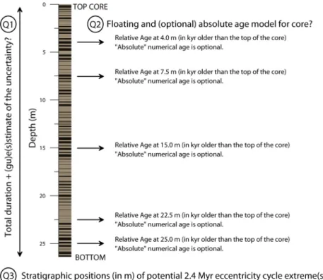
Participants of the CIP received the following information with explanatory text and questions for Case 1 (Fig. 2):
“During the summer of 2027 IODP Expedition 666 “Prelude on the Messinian salinity crisis” successfully recovered a complete and con-tinuous core. The core has a total length of 26.38 m and exists of pelagic carbonate-rich sediments, which look cyclic. Correlations based on seismic profiles and biostratigraphy suggest that the core contains the Tortonian-Messinian boundary around 15-20 m core depth and does not contain any Pliocene material. As the only shipboard cyclostratigrapher, you are asked to look at the color record of the full core and provide the following output to the expedition’s stratigraphic correlator:
Q1: A best estimation on the total duration (in kyr) of the recovered core
based on cyclostratigraphy. What is the uncertainty on this estimation? Do you suspect the presence of any hiatus(es)?
Q2a: A floating age model for following core depths: 4.0, 7.5, 15.0, 22.5
and 25.0 m. [0 m = 0 kyr]. What are the uncertainties on these?
Q2b: Optional: an absolute age model for the same core depths (Tuning).
Uncertainty?
Q3: Stratigraphic positions (in m) of potential 2.4-Myr eccentricity cycle
extreme(s)? Uncertainty?
Data: Information from the introduction and a TIF format color image (Signal_1) of the core (also in separate file).”
2.3. Case 2
2.3.1. Case 2 – motivation and design
Case 2 was designed to represent the following challenges: (a) a non-linear reaction to insolation, as implemented by theImbrie and Imbrie (1980)model, (b) a changing sedimentation rate, (c) a hiatus and (d) auto-regressive (AR1) noise. At the same time, the timing was selected such that the astronomical template (Laskar et al. 2004) is reliable, and effects of tidal dissipation and/or dynamical ellipticity play a negligible role (Lourens et al. 2001;Zeeden et al; 2014). The signal was based on theImbrie & Imbrie (1980)model from 1500-1200 ka and 1000-500 ka, as parametrized for establishing a time scale for a benthic isotope stack (Lisiecki and Raymo, 2005). TheImbrie and Imbrie (1980)model describes non-linear feedback to insolation forcing. It uses a specified feedback time and nonlinearity to model rapid warming and slower cooling. Originally, it was used to model relative ice volume and it is commonly driven by northern hemisphere in-solation. Here, the insolation was mimicked by (Eq.(1)):
= +
+ Mimicked insolation arbitrary units standardized
precession standardized obliquity
[ ] (
[ ] 0.5*
[ ])*11.66 500 (1)
Eq. (1)is based on the suggestion that p-0.5 t (standardized precession minus 0.5 times standardized tilt/obliquity) resembles northern hemisphere insolation, but avoids suggesting a specific forcing latitude (Lourens et al., 1996). This nonlinear dataset was used from 1500-1200 ka and 1000-500 ka, omitting the time from 1200-1000 ka. In a next step the dataset was standardized and combined to reflect a depth series from 0 to 802 (500-1000, 1200-1500) depth units. Subsequently, an up-ramping artificial se-dimentation rate from 1 to 1.5 depth units per cm was applied. The re-sulting dataset was linearly interpolated using (time) steps of 1, rere-sulting in 1002 data points. Finally, 0.5 times standardized auto-regressive noise was added. The change in (artificial) sedimentation rate ranged from 1-1.5 cm kyr-1, which was deliberately lower than a factor of 2, allowing for the
separation of precession- and obliquity components in the power spectrum of the signal in its entirety. The hiatus comprised half of a 405-kyr orbital eccentricity cycle, potentially allowing for its identification through a “too thin” expression of a 405 kyr cycle in the spatial domain. An R script in the Supplementary materials documents the creation of this signal.
2.3.2. Case 2 - assignment
Participants of the CIP received the following information with explanatory text and questions for Case 2 (Fig. 3):
“During the IODP Expedition 999 “Quaternary High Latitudes”, a core showing quasi-cyclic variability in proxy data was recovered. The top-most (and thus top-most recent) sediment is missing for unclear reasons. It is also not clear how much sediment and time is missing. The core has a total length of 10.00 m, and exhibits pattern which seem cyclic. You have a quickly measured record of the magnetic susceptibility (signal origin unclear, but somehow related to paleoclimate/paleoenvironment). Investigation of the biostratigraphy suggests the core to represent sedi-ments with a maximal age of 2 Ma and a minimal age of 0.5 Ma, spanning a maximum time of 1.5 Myr. As cyclostratigrapher you are asked to look at the proxy record of the core, and provide following information:
Q1: A best estimation on the total duration (in kyr) of the recovered core
based on cyclostratigraphy. What is the uncertainty on this estimation? Do you suspect the presence of any hiatus(es)?
Q2a: A floating age model containing for following core positions: 2.0,
4,0, 6.0, 8.0 m. What are the uncertainties on these?
Q2b: Optional: an absolute age model for the same core positions
(Tuning). Uncertainty?
Q3: Stratigraphic positions (in m) of potential 405-kyr eccentricity cycle
extreme(s)? Uncertainty?
Data: Information from the introduction and an Excel data file
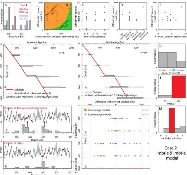
Fig. 3. Case 2 illustration presenting the signal and questions. Additional
stratigraphic information was provided in the accompanying text as well as a data file with the raw data.
(Signal_2) of the record (also in separate file).” 2.4. Case 3
2.4.1. Case 3 – motivation and design
The main challenge for Case 3 was the low signal-to-noise ratio. Moreover, this artificial record represented a much longer duration and was a significantly older sedimentary sequence than Cases 1 and 2. Owing to its age, there are also no theoretical astronomical solutions available for this signal. The signal was based on the output of a general circulation model applied to Late Devonian boundary conditions and runs into steady-state under 31 different astronomical configurations (De Vleeschouwer et al., 2014). The snow cover on Gondwana in austral spring was selected as the input for the signal because this parameter exhibits a highly non-linear response to precession, which is relevant as non-linear responses are also sometimes expressed in the sedimentary rock record. In this Late Devonian scenario, when Earth reach-edperihelion during austral spring, the snow cover on Gondwana melted significantly faster than under other astronomical configura-tions. The 31 snapshot climate simulations were transferred into a
cli-matic time series according to the same procedure that De
Vleeschouwer et al. (2014)followed for surface temperature. The snow-cover time series was truncated to a series that represents 8.703 Myr and was subsequently converted into a stratigraphic series by applying a sedimentation rate with a 1.2-Myr period modulation (Eq.(2)). Lastly, both red and white noise are added to the signal (red noise with mean = 0, sd = 1, lag-1 autocorrelation coefficient = 0.999; white noise with mean = 0, sd = 0.5). The final result is a 394.5 m long stratigraphic series, resampled at 0.15 m intervals. An R script in the Supplementary materials documents the creation of this signal.
= +
SR 4.5 1.5sin 2 t cm kyr
1200 * 1 (2)
2.4.2. Case 3 - assignment
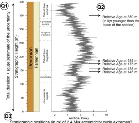
Participants of the CIP received the following information with explanatory text and questions for Case 3 (Fig. 4):
“A team of motivated master students generated a high-resolution (15-cm spaced) proxy record of a 394.5 m thick Late Devonian section in Australia, entirely Famennian in age. The section was deposited in an external carbonate ramp setting. The conodont biostratigraphy of this section is known from the literature, and was constructed based on 40 conodont samples at 10-meter intervals throughout the entire section. Your master students took off to other adventures, and you are left with this exceptionally high-resolution proxy record for the Famennian. Can you distill a cyclostratigraphic story for your next paper?
Q1: A best estimation on the total duration (in kyr) of the recovered core
based on cyclostratigraphy. What is the uncertainty on this estimation? Do you suspect the presence of any hiatus(es)?
Q2: A floating age model for following stratigraphic levels: 145.0, 155.0,
175.0, 185.0, 350.0 m. Output is asked in age, younger than the base of the section. [0 m = 0 kyr]. What are the uncertainties on these? Q3: Stratigraphic positions (in m) of potential 2.4-Myr eccentricity cycle extreme(s)? Uncertainty?
Data: Information from the introduction and a CSV data file (Signal_3) of the record (also in separate file), as well as Fig. 22.10 from the Geological Time Scale 2012, p. 573 (ed.Gradstein et al., 2012) which contains a Late Devonian biostratigraphical framework.”
3. Outcome
3.1. Case 1 – results and observations
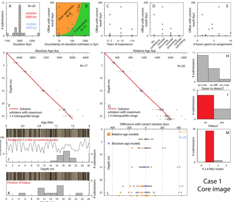
Twenty responses were received that provided analysis of Case 1. The majority (55%) of submitted results for Case 1 reported a total duration estimate that differs less than 1% from the true duration (Fig. 5A). Seven responses were within a 10% error. One duration
Fig. 4. Case 3 illustration presenting the signal and questions. Additional stratigraphic information was provided in the accompanying text as well as a data file with
estimate was 25% too long and one 25% too short. The participants also reported an uncertainty estimate on their duration estimate. When the reported uncertainty was larger than the offset between the reported duration estimate and the true duration, the result was categorized as “conservative” (green background onFig. 5B). When the offset between estimated and true duration was larger than the reported uncertainty, the result was labelled as “over-optimistic” (orange background on Fig. 5B). For Case 1, 40% of the participants produced “over-optimistic” and 60% produced “conservative” results (Fig. 5B). The actual perfor-mance of the participants was also compared to their confidence by using the feedback from the post-conference questionnaire. Participants that expressed higher confidence for Case 1 generally submitted results
closer to the correct solution. This trend is less pronounced for Cases 2 and 3 (Figs. 5D,6D,7D).
Offsets between the submitted and correct total durations versus years of experience (as reported by the participants themselves) suggest an improvement with level of experience (> 10 years) for Case 1 (Fig. 5C). Given the number of participants (20), however, no statisti-cally significant conclusions can be drawn. Note that also in the least experienced group (<5 years) most participants did relatively well (offset <2.5% to correct solution). On average, people spent ∼4.3 hours on Case 1 and no clear improvement of results was seen with increasing study time (Fig. 5E). Except for one participant, re-spondents correctly identified one 2.4-Myr orbital eccentricity
Fig. 5. Case 1 compiled results. (A) Histogram of total duration estimates binned in 50 kyr intervals (N = 20). The red dotted line indicates the correct solution (2000
kyr). The median submitted solution (2000 kyr) is mentioned in blue. (B) Offset between submission and correct solution versus the reported uncertainty on the duration estimate. Green background: reported uncertainty is larger than the offset between the reported duration estimate and the true duration. Orange back-ground: the offset between estimated and true duration is larger than the reported uncertainty. (C) Offset versus the participant’s experience in the general field of cyclostratigraphy. (D) Offset versus the participant’s confidence in his/her analysis of Case 1. (E) Offset versus the amount of time spent on the analysis of Case 1. (F) Submitted absolute age models. The boxplots represent the distributions of the submitted relative ages for five prescribed stratigraphic positions. (G) Submitted relative age models. The boxplots represent the distributions of the submitted relative ages for five prescribed stratigraphic positions. (H) Answers to the question “Which are easier to identify: 2.4-Myr eccentricity minima or eccentricity maxima?” (I) Answers to the question “Did you notice any indication of missing sediment (a hiatus)?”. The correct answer (no) is indicated in red. (J) Participants’ location of the 2.4-Myr orbital eccentricity minimum. (K) Participants’ location of the interpreted hiatus(es). (L) Differences with correct solution between the submitted relative and absolute age models. (M) Answers to the question “How many 2.4-Myr eccentricity minima ("nodes") occur in the analyzed signal”? The correct answer (one) is indicated in red.
minimum (Fig. 5M). The stratigraphic location of this minimum shows variation ranging between 14 and 22 m (Fig. 5J). About 30% of the participants also suggested the presence of one (or more) hiatuses in the record, though no hiatus was introduced in the signal (Fig. 5K). These participants often suspected the hiatus to occur in the 10-12 m and/or the 16-18 m intervals (Fig. 5K). Most placed the hiatus in the 16-18 m interval, which corresponds with low precession and short eccentricity power in the astronomical solution. The weaker expression of the
dominant precession-scale cyclicity in this interval may have “ob-scured” the signal.
Fig. 5F presents the correct solution to Case 1 as an age-depth plot. The boxplots represent the distributions of the submitted relative ages for five prescribed stratigraphic positions. These box plots exhibit a broad total range (outliers and whiskers) but are characterized by a narrow inter-quartile range. Moreover, the median solution accurately approaches the correct solution. In other words, the boxplots visualize the same pattern as Fig. 6. Case 2 compiled results. A) Histogram of the total duration estimates binned in 50 kyr intervals (N = 19). The red dotted line indicates the correct solution
(1000 kyr). The median submitted solution (974 kyr) is mentioned in blue. (B) Offset between submission and correct solution versus the reported uncertainty on the duration estimate. Green background: reported uncertainty is larger than the offset between the reported duration estimate and the true duration. Orange back-ground: the offset between estimated and true duration is larger than the reported uncertainty. (C) Offset versus the participant’s experience in the general field of cyclostratigraphy. (D) Offset versus the participant’s confidence in his/her analysis of Case 2. (E) Offset versus the amount of time spent on the analysis of Case 2. (F) Submitted absolute age models. The boxplots represent the distributions of the submitted relative ages for five prescribed stratigraphic positions. (G) Submitted relative age models. The boxplots represent the distributions of the submitted relative ages for five prescribed stratigraphic positions. (H) Answers to the question “Which are easier to identify: 405-kyr eccentricity minima or eccentricity maxima?” (I) Answers to the question “Did you notice any indication of missing sediment (a hiatus)?”. The correct answer (yes) is indicated in red. (J) Participants’ location of the 405-kyr orbital eccentricity minimum. The red arrows indicate the correct positions of the 405-kyr orbital eccentricity minima. (K) Participants’ location of the interpreted hiatus(es). The red arrow indicates the correct positions of the hiatus. (L) Differences with correct solution between the submitted relative and absolute age models. (M) Answers to the question “How many 405-kyr eccentricity minima ("nodes") occur in the analyzed signal”? The correct answer (two) is indicated in red.
that of the total duration estimates: the distribution of submitted results is characterized by high accuracy but poor precision. Towards the older part of the record, the relative age models exhibit an increasing discrepancy between the correct solution and the submitted results. However, this pattern appears less pronounced for the (tuned) absolute age models, which also have a smaller total error. Different cyclostratigraphic tech-niques probably explain the variation in accuracy between absolute and relative age models for Case 1. Absolute age models are constructed by directly correlating the color record to an astronomical solution or in-solation curve that is expressed in the time-domain, i.e. tuning. The tuning process may have “eliminated” potential small offsets in the relative age models by “rescaling” the record (given the tuning was correct). Inter-estingly, participants chose different tuning targets (e.g. 65 °N 21 June insolation curve, eccentricity curves, precession curves, obliquity curves, combinations of astronomical parameters). The documentation provided by the participants does not give enough detail to convey precise numbers and draw conclusive remarks on the tuning target that leads to the best answers. Yet, the tuning target selection constitutes a relevant aspect of the problem at hand (see discussion on various tuning targets inHinnov, 2018b). One participant actually tuned to the classical 65 °N 21stof June
insolation curve, noted small offsets with the record being investigated and suggested the potential use of a different solution or insolation curve (Case 1 was designed using the 55 °N 21stof July insolation).
In contrast to the two other case studies, Case 1 only provided an image as the data source and not a numerical proxy series. Some par-ticipants directly worked with the image, while others first produced a numerical (color) record for further spectral or other types of digital analysis (or a combination of both). Roughly 3/4 of the participants
chose to digitize the image (with a small number of people using both the image and the numerical color record). Participants who decided to directly work with the image and/or only used visual pattern recogni-tion of the numerical color record (“visual approach”) tended to have smaller errors compared to the other submissions.
3.2. Case 2 – results and observations
Nineteen participants submitted a solution for Case 2. The question on the total duration of the distance-series turned out to be ambiguous. Some participants considered the duration as the time difference be-tween oldest and youngest sediments, and included any missing sedi-ment in this duration (correct answer was 1000 kyr). Others estimated the time contained within only the sediment present (correct answer was 800 kyr). The total duration estimates ranged between 670 and 1500 kyr, which are respectively ∼35 % too short and 50% too long. Despite this large range, the majority of submitted results cluster around the correct answer for the overall duration (maximum age minus minimum age) of sediment present (Fig. 6A). The largest group of participants (7/17) indicated in their report that their duration es-timate was characterized by an uncertainty of ±50 kyr. Shorter and longer uncertainties of (±10 kyr; 5/17 participants) and (±100 or 500 kyr; 5/17 participants) were also reported (Fig. 6A). Most participants (11/17) were over-optimistic in assessing the accuracy of their cyclos-tratigraphic analysis (Fig. 6B). Confidence levels of the submitted re-sults for Case 2 are lower than for Case 1 (Figs. 5D,6D). In Case 2, the accuracy of duration estimates does not exhibit a clear relationship with general experience in cyclostratigraphy (Fig. 6C). On average people Fig. 7. Case 3 compiled results. A) Histogram of the total duration estimates binned in 100 kyr intervals (N = 17). The red dotted line indicates the correct solution
(8703 kyr). The median submitted solution (8800 kyr) is mentioned in blue. (B) Offset between submission and correct solution versus the reported uncertainty on the duration estimate. Green background: reported uncertainty is larger than the offset between the reported duration estimate and the true duration. Orange background: the offset between estimated and true duration is larger than the reported uncertainty. (C) Offset versus the participant’s experience in the general field of cyclostratigraphy. (D) Offset versus the participant’s confidence in his/her analysis of Case 2. (E) Offset versus the amount of time spent on the analysis of Case 2. (F) Submitted relative age models. The boxplots represent the distributions of the submitted relative ages for five prescribed stratigraphic positions. (G) Answers to the question “Which are easier to identify: 2.4-Myr orbital eccentricity minima or eccentricity maxima?” (H) Answers to the question “Did you notice any indication of missing sediment (a hiatus)?”. The correct answer (no) is indicated in red. (I) Answers to the question “How many 405-kyr eccentricity minima ("nodes") occur in the analyzed signal”? The correct answer (four) is indicated in red. (J) Participants’ location of the 2.4-Myr eccentricity minima. The red arrows indicate the correct positions of the 2.4-Myr orbital eccentricity minima.
spent ∼4.7 hours on Case 2 with no clear trend of improvement with increasing study time (Fig. 6E). The majority of participants suggested the presence of a hiatus in this signal (Fig. 6J). Its position was correctly identified by several participants (Fig. 6J), usually the ones using a (visual) direct tuning approach. It is also striking to note that the re-lative age models fall generally close to the solution above the hiatus, while below the hiatus you can distinguish two groups of relative age models with an offset of about the hiatus length (Fig. 6G). Generally, the absolute ages were overestimated by most CIP participants (Fig. 6F), while some provided the correct answers.
The signal of Case 2 deliberately contains four challenges, namely a nonlinear reaction to insolation forcing, an increasing sedimentation rate from 1 to 1.5 cm kyr-1, a hiatus and noise. Most participants used a
combination of visual inspection and statistical analysis for their cy-clostratigraphic analysis. Several interpretations overestimating the duration were based on spectral analysis and filtering of the record, without identifying the change in sedimentation rate. In contrast, the most precise results were based on direct correlation to an insolation target. Several participants correctly assigned the amount of sediment present in terms of time, but did not accurately identify the duration of the hiatus. As may be expected, the hiatus was rather difficult to detect in this signal, although the use of a hiatus that was half a 405-kyr or-bital eccentricity cycle was deliberate since this ensured identification was at least possible. Some participants identified the hiatus during the tuning process. Several participants were unsure about the presence of one (or more) hiatuses, with several suspecting, but not clearly iden-tifying a hiatus. The absence of relationship between years of experi-ence in the general field of cyclostratigraphy and offset to the correct answer is interesting. However, all correct answers were delivered by researchers with experience of working on Neogene cyclostratigraphy, regardless of the total experience in the general field of cyclostrati-graphy in years, and thus familiar with direct tuning of records. The over-optimistic uncertainty assessments may originate from the as-sumptions of an uncertainty of (less than) one interpreted cycle.
3.3. Case 3 – results and observations
Seventeen participants submitted a cyclostratigraphic solution for Case 3. Total duration estimates range between 7.50 and 9.17 Myr, which are respectively ∼15 % too short and 5% too long. Despite this large range, most submitted results cluster around the correct answer (Fig. 7A). Twelve of the submitted durations (12/17, or 71%) fall less than 207 kyr away from the correct solution (i.e. about half a 405-kyr eccentricity cycle), corresponding to an error of less than 2.5%. Most participants indicated that an uncertainty of ±100 or ±500 kyr char-acterizes their duration estimate (Fig. 7B). Thus, most participants correctly assessed the accuracy of their cyclostratigraphic analysis. However, five participants were over-optimistic in their uncertainty estimate and underestimated factors that could negatively impact the accuracy of their cyclostratigraphic analysis. At the other extreme, three participants were overly conservative and indicated a relatively high uncertainties (±500 or ±1000 kyr), whereas their duration esti-mate was offset from the correct solution by less than 10 kyr. The ac-curacy of duration estimates does not exhibit a clear relationship with experience in the general field of cyclostratigraphy (Fig. 7C). On average people spent ∼4.4 hours on Case 3 and no clear improvement of results is observed with increasing study time (Fig. 7E).
The correct solution to Case 3 is presented as an age-distance plot in Fig. 7F. The median solution of the participants’ solutions approaches the correct solution accurately. An individual submitted example is also shown on Fig. 7F, in which the participant constructed a correct age model for the lower 270 m, but then a single cycle is erroneously counted twice, resulting in a ∼400 kyr offset between the correct result and the submitted result. One third to one half of the participants correctly interpreted the stratigraphic position of the two lower 2.4-Myr eccentricity nodes (Fig. 7J). However, the positions of the third and
fourth 2.4-Myr eccentricity nodes were more difficult to detect, as il-lustrated by the spread of submitted positions over the entire upper half of the sequence (Fig. 7J). Detecting 2.4-Myr eccentricity nodes in signal 3 turned out to be quite difficult, with participants observing 2, 3 or 4 nodes. Ten participants correctly presumed that signal 3 is strati-graphically complete, without hiatuses. Seven participants suspected hiatuses.
Case 3 does not contain complications caused by either hiatuses or sudden changes in sedimentation rate. Therefore, the difficulty in analyzing this record lies primarily in the low signal-to-noise ratio. In such a record, the risk of erroneously counting a single cycle twice is rather high, and this is exactly what happened in the example shown in Fig. 7F (9170 kyr), as well as in one other submission (9072 kyr). Si-milarly, two participants missed two or three full 405-kyr cycles in their cycle count, arriving at too short total durations (7500 kyr - 3 cycles missed; 7900 kyr - 2 cycles missed). The largest errors in estimating the total duration of the record are thus caused by mistakes made during the identification of the number of 405-kyr cycles. In that context, it is remarkable that 6 participants indicated that they were convinced of their duration estimate within an uncertainty of ±100 kyr. Such a low uncertainty seems rather optimistic given the risk of counting cycles twice and missing cycles being present in any type of time-series ana-lysis. Indeed, four out of six submissions with such low uncertainty turned out to be over-optimistic.
4. Discussion
4.1. Key lessons learned from the case studies
4.1.1. Reproducibility of results and the importance of integrated stratigraphy
The submitted results and their offsets from the correct solutions should be considered “worst case scenarios” compared to cyclostrati-graphic studies presented in the literature, because there are certain key differences between the CIP case studies and actual published cyclos-tratigraphic studies. Firstly, we should consider the amount of time spent by the participants to investigate these case studies: ∼4.5 hours on average per case ranging from 1.5 hours to more than 10 hours (Figs. 5E,6E, 7E). This is short compared to the time most cyclos-tratigraphers would devote to the interpretation of a record that will end up in a presentation or peer-reviewed publication. Another aspect to consider is that for all three cases, relatively little contextual in-formation and additional stratigraphic constraints were provided. Ide-ally, in a real scenario, a cyclostratigrapher inspects a section or core, samples the succession and integrates his/her analyses with all other sources of information that are available before coming up with an interpretation. Often that researcher will have experience in analyzing coeval strata, and a familiarity with the sedimentology and geological history of the basin that would further help determine the fidelity of the cyclostratigraphic data. A researcher will likely also discuss results and interpretations with colleagues, which will provide an additional feedback loop to critically evaluate output. This is in contrast to the CIP case studies where one of the requirements was to work independently. Moreover, the design of the case studies and the obligation to submit results in a fixed format forced participants to formulate answers that they otherwise might leave more open in a scientific publication, or which would be phrased and discussed rather more carefully and with caveats explored in detail. In many cases, participants signaled that they had only little or moderate confidence in their submitted results (Figs. 5D,6D,7D).
In spite of the range of answers provided by participants, the median of all submissions is in excellent agreement with the correct solution for all three cases. Furthermore, some participants reached the exact correct answer. These results illustrate the power of cyclostrati-graphy as a tool to measure time in geologic sequences: based on the unique imprint of astronomical climate forcing, one can extract
high-resolution geochronologic information and gain insight in the forcing processes behind the environmental change in the geological archive.
4.1.2. Cyclostratigraphy as a trainable skill
The accuracy of submitted results does not seem to improve with increasing level of general experience in the field of cyclostratigraphy. In first instance, this observation may seem problematic, since in-tuitively one expects experienced researchers to do better, and em-phasizing that someone can be trained to become more skilled at in-terpreting cyclostratigraphic data. Equally, however, during in-depth discussions at the CIP meeting, it became clear that experience must be seen in a broader context than just total years (as asked in the ques-tionnaire: “How many years of experience do you have with cyclos-tratigraphy?”). The familiarity with certain types of sedimentary re-cords, datasets and specific stratigraphic time intervals represents the key to more accurate results.
A clear initial distinction exists between records which can be tuned to a robust astronomical solution (Cases 1 and 2) and those for which no correlation template is available (Case 3). Discussions during the CIP meeting clearly highlighted that people with experience in astronom-ical tuning to astronomastronom-ical solutions did better in Case 1 and 2, whereas participants with more experience in the astronomical calibration of floating chronologies for which no astronomical solutions are available performed better in Case 3. This is a crucial observation demonstrating that the quality of cyclostratigraphic analyses depends to some extent on past experience with similar datasets, and that one can improve their results by acquiring more experience with relevant studies.
4.2. Uncertainties in cyclostratigraphy in the light of the CIP
The reconstructed total signal durations clustered around the exact solution for Cases 1 and 3 (Figs. 5A,7A), complemented by a handful of outliers. For Case 2, where the data contained a hiatus, the total duration estimates have a bimodal distribution (Fig. 6A; see Section 3.2). The CIP results further show that cyclostratigraphers rather poorly self-estimate the uncertainties of their analysis, as only a weak corre-spondence is observed between self-estimated uncertainty and the ac-tual offset of the submitted result with the true duration. This might also be due to the limited available stratigraphic constraints that were provided. In Case 1, the accuracy of the proposed duration was sys-tematically higher when the methodology relied on visual analysis ra-ther than on statistical approaches. Furra-thermore, age models tuned to astronomical solutions (Cases 1 and 2) are more accurate compared to floating time scales (Case 3). We interpret the success of the visual tuning approach in Case 1 as an illustration of the importance of clear observations and a robust plausible astronomical interpretation before pursuing any form of statistical analysis. Hence, this underlines the importance of training in recognizing regular sedimentary patterns and formulating different interpretations for their origin.
At present, cyclostratigraphic studies do not report uncertainty in a systematic way. When discussing “uncertainty”, we do not refer here to the significance testing for the possible presence or absence of an as-tronomical imprint in a signal (e.g. sensuHuybers and Wunsch, 2005; Meyers and Sageman, 2007;Meyers, 2015;Li et al., 2018), but instead to the reported uncertainties on astrochronologic ages and durations derived from the cyclostratigraphic analysis. Several studies have dealt with uncertainty by documenting different tuning options (e.g. Westerhold et al., 2008; Lauretano et al., 2016; Drury et al., 2017) while others have provided a quantitative estimate of uncertainty (e.g. Kuiper et al., 2008;Rivera et al., 2011;Zeeden et al., 2014). New sta-tistical techniques also allow for uncertainties to be estimated on re-constructed sedimentation rates (e.g., ACEv1, Sinnesael et al., 2016; TimeOptMCMC,Meyers and Malinverno, 2018). Nonetheless, no spe-cific established method is yet accepted as a standard and the most explicit quantification of uncertainty on astrochronologic results has been attempted in studies focusing on the intercalibration of
cyclostratigraphy with radioisotopic dating (Kuiper et al., 2008;Rivera et al., 2011;Meyers et al., 2012;Sageman et al., 2014;Zeeden et al., 2014). Progress is often made by starting from existing astro-chronologies and either confirm, adjust or improve them.
The intercalibration with other geochronometers is essential to evaluate uncertainty. This only holds in the case when geochron-ometers are not used to calibrate the age model in any way, avoiding circular reasoning. Using an integrated stratigraphic approach may highlight potential inconsistencies with astrochronologic duration es-timates of certain stratigraphic intervals (e.g. hiatuses or splice pro-blems). Integrated stratigraphy should be used to confirm, or challenge astronomical interpretations, wherever possible. However, when in-dependent geochronological information is insufficient to narrow down different astrochronologic interpretations, the documentation of mul-tiple astrochronologic interpretations appears to be the best option. Instead of the common practice of reporting a rather arbitrary number of cycles as an uncertainty estimate, we encourage cyclostratigraphers to shift the focus of the uncertainty assessment towards the source of uncertainty (e.g. band pass filter settings, potential changes in sedi-mentation rates, likelihood of hiatuses). When the completeness of a record is not guaranteed by means of a sufficiently detailed in-dependent stratigraphic framework, authors should report duration estimates as minimum estimates (e.g.Weedon et al., 2019). The dis-cussion of these aspects provides the reader with a better insight into the potential size of uncertainties on the astrochronology presented, and provides some clear targets for future improvement.
4.2.1. Uncertainties of records tuned to astronomical solutions
An obvious source of age-distance model uncertainty for tuned time-scales relates to the choice of tuning target. This issue is illustrated by the variety of tuning targets that were used by participants to solve the first two cases. Indeed, we used an “unconventional” input of the 55 °N 21stJuly insolation when constructing Case 1 to raise awareness of this
issue. For records older than ∼10 Ma, an additional source of un-certainty arises from unknown changes in past tidal dissipation and/or dynamical ellipticity (e.g.Laskar et al. 2004;Zeeden et al. 2014). Un-certainty also commonly arises from the choice of climate/ice sheet model response, proxy-target phase relationship (which can change over time) and the interpolation between tuning tie points, which mainly acts at the scale of the period of the smallest cycle used for tuning (e.g. Beddow et al., 2018; Liebrand et al., 2016). Most im-portantly, the correctness of the identification of astronomical cycles in the geological record is a critical factor, affecting tuned and untuned age-depth models alike. In the Neogene, integrated stratigraphic ap-proaches, also based on magnetostratigraphy, biostratigraphy and radioisotopic dating, or where successions from multiple locations are compared, can support correct cycle identification in many cases (an-chored astrochronologies tuned to astronomical solutions).
4.2.2. Uncertainties of astrochronologies without astronomical solutions
While most Cenozoic and late Mesozoic (only considering the stable 405-kyr eccentricity cycle) astronomical time scales can be based on direct correlation/tuning to an orbital astronomical target, for older intervals of the stratigraphic column direct calibration to an astro-nomical target curve is not possible and one has to construct so-called “floating” and “anchored” astronomical age models (see Section1. In-troduction). For the construction of “floating” and “anchored” astro-nomical age models when a reliable astroastro-nomical solution is absent, astronomically-forced (climate) signals are typically extracted from the rock record and their cyclic character is interpreted in terms of astro-nomical forcing using a number of approaches. Ratios of the periods of identified spectral peaks in the spatial domain, often in combination with independent age/duration estimates based on bio-/magnetos-tratigraphic and/or radioisotopic dating allow for the identification of the main cycles in the data (Hays et al., 1976;Meyers and Sageman, 2007;Li et al., 2018). Amplitude modulations of high-frequency cyclic
components can serve to extract the phase relationship to low-fre-quency eccentricity or obliquity amplitude modulations (e.g. Shackleton et al., 1995;Zeeden et al., 2015;Meyers, 2015;Laurin et al., 2016). When the main beat of the record is identified, an average cycle duration can be assumed (e.g. 405-kyr for the stable long eccentricity cycle) and a floating time scale can be anchored with respect to a re-ference point, such as the base of a section, a radioisotopic age, or a numeric age defined biostratigraphically (e.g. the Frasnian-Famennian boundary inDe Vleeschouwer et al., 2017b). This approach is partly arbitrary since when one “counts cycles” the precise duration one uses for a certain period has a significant impact on the estimated total duration. For example, if one counts a number of Quaternary precession cycles and multiplies this number with their duration, assuming a duration of 20 kyr instead of, for example, 21 kyr results in a 5% offset for a floating age model. Another typical source of uncertainty is the number of cycles one identifies in a record.
In none of the three CIP cases did participants uniformly locate eccentricity minima in the provided records. Yet, most participants indicated that eccentricity minima are easier to detect than eccentricity maxima (Figs. 5I,6I,7G). The identification of the position of relative extremes in any type of cycle is a non-trivial issue, as they are often used for correlation and tuning purposes. However, the cyclostrati-graphic community has yet to define such extremes unambiguously: Is it one specific level or a certain interval? Is it the zone of the least clear development/expression of precession cycles? Is it where a 2.4-Myr orbital eccentricity bandpass filter is lowest? In that case, what would be the appropriate band pass filter settings? A common understanding and agreement on the concept of the identification of relative extremes is important and would also contribute to the reproducibility of cy-clostratigraphy and astrochronology. The definition of orbital extremes remains a relevant topic, which requires further discussion.
In contrast to Cases 1 and 2, no theoretical astronomical solution was available for Case 3. Signals filtered for the 405-kyr eccentricity cycle resulted in different numbers of cycles between 275 and 330 m, where the record had a reduced signal-to-noise ratio. Here, depending on the filter parameters used (especially the filter width), either 4 or 5 cycles were recognized in the filtered signal. The correct number of cycles (4 cycles) could be determined by considering not only the 405-kyr cycles, but also the shorter cycles (100-405-kyr eccentricity, obliquity and precession). If a 405-kyr eccentricity cycle is counted twice, it re-sults in a distorted spectrum for the interval that does not fit perfectly with the expected astronomical ratios between spectral peaks. For this reason, we argue that evolutionary analysis methods should be used (i.e. sliding window spectral analysis or wavelet analysis), both in the spatial- and time-domain, before and after the construction of a floating astrochronologic age-depth model.
4.3. Recurrent points of discussion in cyclostratigraphy in the light of the CIP
During the three-day CIP meeting in Brussels, several outstanding issues in cyclostratigraphy were discussed. In this section, we sum-marize the outcome of those discussions and relate them to the case studies where possible.
4.3.1. Visual and numerical cyclostratigraphy
An important discussion in cyclostratigraphy revolves around the merits and pitfalls of numerical/statistical versus visual cycle-pattern recognition approaches. The CIP allows for a direct comparison of re-sults obtained through both approaches, although in practice many participants combined the two. The statistical approach uses numerical methods to identify and analyze (quasi)cyclic patterns, and in some cases applies automated procedures to correlate proxy records to se-lected astronomical target curves for tuning. The visual approach uses a manual inspection of characteristic cycle patterns for identification and interpretation as well as for matching records to astronomical target
curves.
A large number of participants successfully applied the visual ap-proach in Cases 1 and 2, and in several cases derived the correct an-swer. The method is frequently combined with results of numerical analysis, in particular with spectral techniques to identify cycles in a statistically meaningful way which are then combined with bandpass filtering. For this purpose, about 75% of the participants created quantitative records of the lithologic log in Case 1 through color-greyness analysis. However, tuning to astronomical target curves was in all attempted cases (as far as documented) achieved through pattern matching and not via automated correlation procedures. The latter could also be due to the relatively limited amount of time spent on the exercises (∼4.5 hours on average), in combination with inexperience of the participants with automated correlation procedures and docu-mented issues induced by automated methods (Hilgen et al., 2014). The visual approach, also repeatedly used in the more complex Case 2, led in some instances to correct answers. However, pattern matching sug-gested that a second tuning option with two hiatuses existed, which, although showing a poorer fit, could not be fully excluded by partici-pants. Purely numerical attempts to identify the hiatus proved less successful. These numerical attempts were based on the splitting of spectral peaks in evolutive spectra, but the presence of multiple spectral peaks can also result from the added noise. Furthermore, until recently the visual approach was the only explicit approach dealing with am-plitude modulations in a signal. Recently, two approaches were pub-lished, which use amplitude variations for astronomical time scale construction (Meyers, 2015, 2019) and for testing tuned time scales (Zeeden et al., 2015,2019).
The results show that Cases 1 and 2 can in principle be carried out without applying any numerical methods or statistics, leading to cor-rectly tuned age models. This is not only the case for the relatively straightforward Case 1, but also for the more complicated Case 2 in-cluding the hiatus. A visual or combined visual-statistical approach was rarely applied to the late Devonian Case 3. Nonetheless, a critical comparison of numerical results, e.g. bandpass filters and spatial/time evolutive methods, with a visual inspection of the record is important for detecting unwanted side effects of some numerical methods.
Bandpass filtering has the potential to give insight into the time-evolutive amplitude in a specific bandwidth. Commonly, the filtered frequency band is chosen rather arbitrarily and the details are not al-ways reported, which hampers reproducibility. A recent study carried out an extensive search for optimal Taner (Taner, 1992) bandpass filters for cyclostratigraphy (Zeeden et al., 2018). The general advice re-garding the filtering of stratigraphic records in the spatial domain (e.g. using Taner or Gaussian filters), is to select a filter that comfortably encompasses the frequency range of the targeted cycle in the depth domain but does not overlap with the frequency range of a neigh-bouring astronomical parameter. It is important that during the com-parison of the bandpass filter output and the original data, the user identifies intervals in the proxy records where one runs the risk of counting a specific cycle in the proxy record twice, or, contrarily, where the filter merged two cycles in the proxy records (causing an under-estimation of the number of cycles). Indeed, minor changes in bandpass filter design can lead to different filter outputs and a variable total number of cycles picked up by the filter. In Case 3, the identification of a different number of 405-kyr cycles occurs between 260 and 320 m, where the noise in the signal makes the detection of the astronomical signal particularly difficult. Another numerical approach to extract as-tronomical components from a record is to use polynomial modelling of a spectral frequency range (e.g. ACEv1: Sinnesael et al., 2016), or through frequency domain period tracking (Park and Herbert, 1987; Meyers et al., 2001). To increase the potential for reproducible cy-clostratigraphy, it is recommended to keep a detailed record of applied methods and to clearly report specific bandpass filter settings.