Summertime elemental mercury exchange of temperate grasslands on an ecosystem-scale

(1)

HAL Id: hal-00303279

https://hal.archives-ouvertes.fr/hal-00303279

Submitted on 4 Feb 2008

HAL is a multi-disciplinary open access

archive for the deposit and dissemination of sci-entific research documents, whether they are pub-lished or not. The documents may come from teaching and research institutions in France or abroad, or from public or private research centers.

L’archive ouverte pluridisciplinaire HAL, est destinée au dépôt et à la diffusion de documents scientifiques de niveau recherche, publiés ou non, émanant des établissements d’enseignement et de recherche français ou étrangers, des laboratoires publics ou privés.

Summertime elemental mercury exchange of temperate

grasslands on an ecosystem-scale

J. Fritsche, G. Wohlfahrt, C. Ammann, M. Zeeman, A. Hammerle, D. Obrist,

C. Alewell

To cite this version:

J. Fritsche, G. Wohlfahrt, C. Ammann, M. Zeeman, A. Hammerle, et al.. Summertime elemental mercury exchange of temperate grasslands on an ecosystem-scale. Atmospheric Chemistry and Physics Discussions, European Geosciences Union, 2008, 8 (1), pp.1951-1979. �hal-00303279�

(2)

ACPD

8, 1951–1979, 2008 Mercury exchange of temperate montane grasslands J. Fritsche et al. Title Page Abstract Introduction Conclusions References Tables Figures ◭ ◮ ◭ ◮ Back Close

Full Screen / Esc

Printer-friendly Version Interactive Discussion

Atmos. Chem. Phys. Discuss., 8, 1951–1979, 2008 www.atmos-chem-phys-discuss.net/8/1951/2008/ © Author(s) 2008. This work is licensed

under a Creative Commons License.

Atmospheric Chemistry and Physics Discussions

Summertime elemental mercury exchange

of temperate grasslands on an

ecosystem-scale

J. Fritsche1, G. Wohlfahrt2, C. Ammann3, M. Zeeman4, A. Hammerle2, D. Obrist5, and C. Alewell1

1

Institute of Environmental Geosciences, University of Basel, Bernoullistrasse 30, 4056 Basel, Switzerland

2

Institute of Ecology, University of Innsbruck, Sternwartestrasse 15, 6020 Innsbruck, Austria 3

Agroscope Reckenholz-Taenikon Research Station ART, Air pollution/Climate group, Reckenholzstrasse 191, 8046 Zurich, Switzerland

4

Institute of Plant Science, ETH Zurich, Universitaetsstrasse 2, 8092 Zurich, Switzerland 5

Desert Research Institute, Division of Atmospheric Sciences, 2215 Raggio Parkway, Reno, NV 89512, USA

Received: 1 October 2007 – Accepted: 8 January 2008 – Published: 4 February 2008 Correspondence to: J. Fritsche ([email protected])

(3)

ACPD

Full Screen / Esc

EGU

Abstract

In order to estimate the air-surface mercury exchange of grasslands in temperate cli-mate regions, fluxes of gaseous elemental mercury (GEM) were measured at two sites in Switzerland and one in Austria during summer 2006. Two classic micrometeorolog-ical methods (aerodynamic and modified Bowen ratio) have been applied to estimate

5

net GEM exchange rates and to determine the response of the GEM flux to changes in environmental conditions (e.g. heavy rain, summer ozone) on an ecosystem-scale. Both methods proved to be appropriate to estimate fluxes on time scales of a few hours and longer. Average dry deposition rates up to 4.3 ng m−2h−1and mean deposi-tion velocities up to 0.10 cm s−1 were measured, which indicates that during the active

10

vegetation period temperate grasslands are a small net sink for atmospheric mercury. With increasing ozone concentrations depletion of GEM was observed, but could not be quantified from the flux signal. Night-time deposition fluxes of GEM were measured and seem to be the result of mercury co-deposition with condensing water. Effects of rain and of grass cuts could also be observed, but were of minor magnitude.

15

1 Introduction

The continued use of mercury in a wide range of products and processes and its re-lease into the environment lead to exposition of mercury in ecosystems yet unspoiled. Its long atmospheric lifetime of about 1 to 2 years (Lin and Pehkonen,1999) enables elemental mercury (Hg0) to migrate to remote areas far away from its emission source,

20

and once deposited to terrestrial or aquatic surfaces it is exposed to the formation of even more toxic methylmercury (IOMC,2002). A suite of factors determines the ulti-mate fate of elemental mercury and its eventual immobilisation at the Earth’s surface. Depending on atmospheric chemistry, meteorological conditions and physicochemical properties of the soils mercury may be cycled fairly rapidly between terrestrial surfaces

25

(4)

ACPD

Full Screen / Esc

deposited mercury is retained in background soils or whether terrestrial surfaces are even a net source of mercury (Pirrone and Mahaffey, 2005). Once deposited, mer-cury may be sequestered (e.g. adsorbed to soil organic matter and clay minerals), re-moved from the soil by leaching and erosion or re-emitted (Gustin and Lindberg,2005). Mercury sequestered by terrestrial ecosystems might eventually be disconnected

tem-5

porarily from the atmosphere-biosphere cycle, which would lead to a decrease in the pool of atmospheric mercury.

The function of vegetation in the mercury exchange with the atmosphere remains unclear. Mercury may be taken up by leaves or transferred from the soil through the plant to the atmosphere (Gustin and Lindberg, 2005; Millhollen et al., 2006). Foliar

10

uptake has been suggested to be an important pathway for atmospheric mercury to enter terrestrial ecosystems and may represent a significant, but poorly quantified sink within the biogeochemical cycle, possibly accounting for over 1 000 tons of mercury per year (Obrist,2007). Du and Fang (1982) measured Hg0uptake of several C3 and C4 plant species and demonstrated that stomatal and biochemical processes control

15

the uptake. Atmospheric mercury concentration was found to be the dominant factor associated with foliar mercury concentrations in different forb species (Fay and Gustin, 2007), and the successful application of different grass species in biomonitoring stud-ies (De Temmerman et al.,2007) suggest that mercury uptake by plants is indeed of significance.

20

With innovations in sensitive measurement techniques in the last decade it is now possible to measure atmospheric mercury background concentrations currently rang-ing from 1.32 to 1.83 ng m−3 ₍_{Valente et al.}_, ₂₀₀₇_{). Such instruments also allow the}

estimation of air-surface exchange fluxes of gaseous elemental mercury (GEM) by ap-plying micrometeorological methods. They are based on vertical concentration profiles

25

and permit spatially averaged measurements without disturbing ambient conditions – an essential element of long-term studies.

During our previous work on GEM exchange of a montane grassland in Switzerland we determined mean deposition rates of 5.6 ng m−2h−1 during the vegetation period

(5)

ACPD

Full Screen / Esc

EGU (Fritsche et al., 2008). In the current study that work is extended to another

mon-tane and one lowland grassland site along the Alps with the aim to determine whether all temperate grasslands are net sinks for atmospheric mercury or whether GEM ex-change is site specific. Two classical micrometeorological methods are applied to es-timate the GEM fluxes: the aerodynamic method and the modified Bowen ratio (MBR)

5

method. By performing these measurements during the vegetation period, we also attempt to capture changes in the GEM flux caused by alteration of environmental conditions, e.g. grass cuts, heavy precipitation, and elevated summer ozone concen-trations.

2 Experimental

10

2.1 Site description

For our GEM flux measurements we selected three grassland sites in Switzerland and Austria with existing micrometeorological towers. The first site, Fruebuel, is located on an undulating plateau 1 000 m a.s.l. in central Switzerland. It is intensively used for cattle grazing and is bordered by forest, wetlands and other grasslands. The second

15

location, Neustift, is an intensively managed, flat grassland in the Austrian Stubai Val-ley at an elevation of 970 m a.s.l. This previously alluvial land lies between the Ruetz river and pastures and is primarily used for hay production. The third site is situated in Oensingen on the Swiss central plateau (Mittelland) at 450 m a.s.l. between the Jura and the western Alps. It serves as an experimental farmland with extensive

manage-20

ment and neighbours agricultural land that borders on a motorway in the north-west. All three sites are equipped with eddy covariance (EC) flux towers. The stations in Neustift and Oensingen are affiliated with the CarboEurope CO2 flux network and are

operated by the Institute of Ecology, University of Innsbruck, Austria and the Federal Research Station Agroscope ART, Switzerland, respectively. At Fruebuel the EC flux

25

(6)

green-ACPD

Full Screen / Esc

house gas fluxes from agricultural land in the context of a changing climate.

Details about the meteorological and pedological conditions of all three sites are listed in Table1. The predominant wind direction at Fruebuel is SW to SSW, showing a distinct channelled flow as a result of the local, undulating, sub-alpine topography. The largest contributions to the footprint are within approximately 60 m of the eddy

5

covariance tower. Neustift on the other hand represents a site with the characteristic wind regime of an Alpine valley – the wind blowing into the valley from NE during the day and blowing out of the valley from SW during the night. Vegetation is uniform for around 300 and 900 m in the directions of the day- and night-time winds, respectively, with the footprint maximum lying within these boundaries for more than 90% of all

10

cases. In Oensingen the fetch length is about 70 m along the dominant wind sectors (SW and NE) and 26 m in the perpendicular axis. The fraction of the field contributing to the measured EC CO2flux is>70% during most of the daytime, whereas during

night-times, this fraction is generally lower and highly variable due to very stable conditions. The gleyic cambisols at Fruebuel and the stagnic cambisols at Oensingen are rather

15

deep (>1 m), while the gleyic fluvisol in Neustift is very shallow (<30 cm). Total mercury

concentrations at all sites are representative of uncontaminated background soils (see Table 1), although the Hgtot concentration at Fruebuel lies at the threshold value of

100 ng g−1. We performed our measurements between June and September 2006 for two weeks at each site.

20

2.2 Micrometeorological methods

A variety of micrometeorological techniques to estimate atmosphere-surface exchange fluxes of trace gases have been developed (Dabberdt et al., 1993;Lenschow,1995; Baldocchi, 2006; Foken, 2006). Of these, the eddy covariance approach would be most straightforward, but is currently not feasible for GEM as no fast-response sensor

25

is yet available (Dabberdt et al.,1993;Lindberg et al.,1995). We therefore resorted to two more empirical methods. The first, the aerodynamic technique, is an application of Fick’s law of diffusion to the turbulent atmosphere (Baldocchi,2006). Translated to an

(7)

ACPD

Full Screen / Esc

EGU atmospheric trace gas the general relationship for the flux is

Fx = −Kx

∂c_x

∂z (1)

whereF_x is the vertical trace gas flux, K_x the eddy diffusivity and∂c_x/∂z the

con-centration gradient of an arbitrary, non reactive trace gas x (Dabberdt et al., 1993; Lenschow, 1995; Baldocchi,2006). Corresponding equations have been formulated

5

for the momentum flux (Q_M) as well as the fluxes of sensible (Q_H) and latent heat (Q_E). It is assumed that the sources and sinks of these scalars are equal and thus similarity between the eddy diffusivities (K_x=_K_H =_K_E_{) are implied.}

The eddy diffusivityK_x is expressed by the aerodynamic method as

K_x = k × u∗× z

Φ_h₍_z/L) (2)

10

wherek denotes the von Karman constant (0.4), u_∗ the friction velocity,z the

mea-surement height, Φ_h(z/L) the universal temperature profile and L the Monin-Obukhov

length. Generally the eddy covariance technique is used to determine the friction ve-locity andL is calculated from u_∗, air temperature, air density and the sensible heat flux. By combination of Eq. (1) and (2) and subsequent integration we obtain

15

FGEM = −

k × u_∗× (cGEMz₂− cGEMz₁)

log(z2/z1) +ψz₂− ψz₁

(3)

whereψ_z₁ and ψ_z₂ are the integrated similarity functions for heat at the measured heights. A more detailed description of this method is given inEdwards et al.(2005).

The second method employed is the modified Bowen ratio method, which is a slightly more direct technique to estimate the GEM flux. This method uses directly measured

20

(8)

ACPD

Full Screen / Esc

gradient of this scalar. In our studies we measured the fluxes of CO₂with eddy covari-ance and its vertical gradient concurrently with the GEM gradients. The GEM flux is then calculated as FGEM =FCO₂× ∆_c_GEM ∆_c_CO 2 (4)

Further details and previous applications of this method are described by e.g.Meyers

5

et al. (1996) andLindberg and Meyers(2001). 2.3 Instrumentation

Air concentrations of GEM were measured in 5-min intervals with a dual cartridge mer-cury vapour analyser (Tekran 2536A, Tekran, Toronto, Canada). With this instrument mercury is preconcentrated by amalgamation and detected via cold vapour atomic

10

fluorescence spectrometry; further details of its operation principals are described in e.g.Lindberg et al. (2000). The instrument was calibrated automatically every 24 h by means of an internal mercury permeation source. Additional, manual calibrations were performed prior to each measurement campaign by injecting mercury vapour with stan-dard gas tight syringes from a mercury vapour generation unit (Model 2505, Tekran,

15

Toronto, Canada).

In order to compute GEM fluxes by the MBR method CO₂concentrations were mea-sured with a closed path infrared gas analyser (LI-6262, LI-COR Inc., Lincoln, Ne-braska, USA) at a frequency of 1 Hz. Before each campaign the gas analyser was calibrated with argon as zero gas and pressurised air with 451 ppm CO₂as span gas.

20

The zero-offset of argon relative to a N2/O2gas mixture was 0.4 ppm.

Meteorological data (air temperature, net radiation, PAR, humidity, wind speed, wind direction) were recorded by the micrometeorological instrumentation of the towers at the study sites. Carbon dioxide and water vapour fluxes were determined by eddy covariance using three-dimensional sonic anemometers and open path infrared gas

(9)

ACPD

Full Screen / Esc

EGU analysers (Solent R2 and R3 [Gill Ltd., Lymington, UK] and LI-7500 [LI-COR Inc.,

Lin-coln, Nebraska, USA]). 2.4 Measurement setup

Vertical concentration gradients were determined by measuring GEM and CO2 at

5 heights above ground (0.2, 0.3, 1.0, 1.6 and 1.7 m). The same setup was installed

5

at all three sites, although the lowest sampling heights had to be adjusted to the local height of the vegetation (10–60 cm at Fruebuel and Neustift, and 10–20 cm at Oensin-gen). The sampling lines consisting of 1/4”-tubing were mounted to a mast in the vicinity of the micrometeorological towers and connected to a 5 port solenoid switching unit. Depending on space and the setup of the micrometeorological equipment at each

10

site, the sampling lines were between 7 and 15 m long (all lines at each site had equal length). Downstream of the switch unit, the Tekran instrument and the CO2 analyser

were connected in series. Filter cartridges with 0.2µm Teflon filters were mounted to

the inlets of the sampling lines to prevent contamination of the analytical system. Tub-ing and fittTub-ings made of Teflon were used and cleaned with HNO3and deionised water

15

according to an internal standard operating procedure (adapted fromKeeler and Lan-dis,1994). The system was checked for contamination by measuring mercury-free air generated by a zero air generator (Model 1100, Tekran, Toronto, Canada). Additionally, by constricting the sampling lines temporarily it was tested if the setup had any leaks.

Air was sampled at a flow rate of 1.5 l min−1 by the internal pump of the Tekran

20

instrument. To maintain continuous flushing of all sampling tubes an auxiliary pump with a flow rate of 6.0 l min−1 was connected to the four lines that were currently not sampled. The sampled air was not dried, which required correction of the calculated fluxes for density effects (see below).

Air sampling was switched from a line at a lower height to one at an upper height

25

every 10 min (i.e. the sequence with the heights mentioned above was 0.2–1.6–0.3– 1.7–1.0 m). In this way a vertical concentration profile with five measurement points could be determined every 50 min. Higher frequencies were not feasible as the low

(10)

ACPD

Full Screen / Esc

ambient GEM concentrations require pre-concentration by the gold cartridges of the Tekran intrument for accurate analysis.

2.5 Flux calculations

Upon completion of the measurement campaigns, GEM and CO2 fluxes were

com-puted with a self-programmed Matlab® algorithm. Carbon dioxide fluxes were

calcu-5

lated to evaluate the quality of the GEM fluxes. By comparing the CO2 fluxes

deter-mined by the aerodynamic method with the CO2 fluxes obtained by eddy covariance

we could assess the reliability of the aerodynamic method, i.e. matching CO₂ fluxes lend credibility to the calculated GEM fluxes (assuming the CO2 fluxes determined by

EC to be accurate).

10

After correction of the GEM and CO₂ concentrations with respect to the measured standards the atmospheric concentration trend was subtracted from the data by in-terpolating the concentration measured at the top sampling line to the measurements of the other lines. This step was considered essential as atmospheric concentrations changed during the course of a measurement cycle of 50 min (i.e. 20 min for one height

15

pair) and overlaid the measured gradients. Next, GEM and CO2fluxes were calculated

according to Eq.3and4for four successive height pairs per measurement cycle. The raw fluxes were then obtained by computing the median of these four values, thus reducing uncertainty substantially.

As the sampled air was not dried the raw fluxes were corrected for density effects of

20

water vapour according toWebb et al.(1980). A correction for sensible heat was not considered necessary, because the sample air of all lines was brought to a common temperature before reaching the analysers and because the Tekran instrument moni-tors the GEM concentration relative to the sampled air mass with a mass flow controller. Finally, the GEM and CO2flux data were screened for outliers and values outside the

25

(11)

ACPD

Full Screen / Esc

EGU

3 Results

3.1 Data coverage

We performed our measurements at the three sites under fair weather conditions. How-ever, due to power outages and showers during thunderstorms as well as instrument failures, not all variables required to calculate the GEM and CO2fluxes could be

mea-5

sured continuously. As shown in Table1GEM fluxes could be computed for up to 85% of the measurement periods. In Neustift and Oensingen the data coverage of the GEM fluxes calculated by the MBR method was considerably reduced due to failure of the eddy covariance systems.

As the resolution of gradient measurements is limited we determined the minimum

10

resolvable gradient (MRG) in a similar way as described byEdwards et al.(2005). This was done at Fruebuel by mounting all five sampling lines at 1 m above ground, measur-ing the GEM and CO₂ concentrations for three days and computing the concentration differences between the line pairs used for the flux calculations. By defining the MRG as the mean of the concentration differences plus one standard deviation we obtained

15

MRG’s of 0.02 ng m−3 _{for GEM and 2.5 ppm for CO}

2. This translates to minimum GEM

fluxes determinable with the aerodynamic method of −2.8 to −4.6 ng m−2 h−1for typ-ical daytime and −0.5 to −1.9 ng m−2 h−1 for typical night-time turbulence regimes (for daytime u_∗=0.17 to 0.27 m s−1 _and _{z/L=−0.49 to −0.16; for night-time u}

∗=0.032

to 0.11 m s−1 _and _{z/L=2.2 to 0.15 [data from the Fruebuel site]). Excluding outliers}

20

and flux values with gradients below the MRG, the overall data coverage for the GEM fluxes at the three sites was between 27 and 58% (see Table1 for details). However, exchange rates calculated with smaller gradients than the MRG were included in the results reported below, as average fluxes would otherwise be overestimated.

(12)

ACPD

Full Screen / Esc

3.2 Meteorological conditions

Meteorological conditions at the three sites were mainly sunny and stationary most of the time (see Fig.1to 3and Table 1). The measurement campaign in Oensingen was scheduled for September 2006 when air temperature and irradiation were some-what lower than at the other sites. However, conditions in Oensingen were unstable

5

and very humid with evening and night-time thunderstorms. Atmospheric turbulence at Fruebuel and Neustift was very similar with average values of 0.17 m s−1_{. The value for}

Oensingen was lower with 0.12 m s−1. At the national air monitoring stations nearest to Fruebuel and Oensingen average O3concentrations of 123 and 25µg m−3,

respec-tively, were measured during the study periods.

10

3.3 Atmospheric GEM concentrations

Average atmospheric GEM concentrations measured 1.7 m above ground were 1.2±0.2 ng m−3 at both, the Fruebuel and Neustift sites, and 1.7 ±0.5 ng m−3 at the site in Oensingen (see Table1). The highest concentration was measured in Oensin-gen during daytime with 4.7 ng m−3, the lowest in Neustift with 0.5 ng m−3 during the

15

night (see Fig. 1 to 3). As can be seen in Fig. 4 the concentrations in Neustift and Oensingen followed a distinct diurnal pattern with lowest GEM concentrations in the af-ternoon between 14 and 15 h. This pattern was particularly pronounced in Neustift with an average diurnal amplitude of 0.32 ng m−3. In contrast, a diurnal signal at Fruebuel was absent and concentrations nearly constant.

20

Calculation of the correlation coefficients between ambient GEM concentration and meteorological variables revealed moderate linear relationships with relative humidity and atmospheric O₃ at Fruebuel and Oensingen (see Table2). More pronounced cor-relations of GEM concentration were detected in Neusitft for most variables, notably air temperature and PAR, but no O3record was available for this site.

(13)

ACPD

Full Screen / Esc

EGU 3.4 CO₂and GEM fluxes

In Table 1 a summary of the average GEM and CO2 gradients and fluxes is given

for the investigated sites; the corresponding time series are shown in Fig. 1 to 3. Due to large spread, fluxes and GEM gradients were smoothed with a 9-point mov-ing average (which corresponds to an interval of ∼8 h). As expected, the

verti-5

cal concentration gradients and fluxes of CO₂ varied substantially between day and night. While the highest average day-time gradient (9–15 h) was recorded at Fruebuel with 9.3 ppm m−1, the highest average night-time gradient (23–5 h) was measured in Neustift with −43 ppm m−1. The largest gradient of −220 ppm m−1 was measured at Oensingen during one night.

10

As mentioned in the experimental section CO2fluxes were determined two-fold, with

eddy covariance and the aerodynamic method. The former yielded on average a net uptake or deposition of 6.4µmol m−2_s−1_{and 5.3}_{µmol m}−2_s−1_{at Fruebuel and}

Oensin-gen, respectively, and a mean net CO2 emission of 3.6µmol m−2s−1 in Neustift. With

the aerodynamic method average deposition of 5.4µmol m−2_s−1_{and 1.7}_{µmol m}−2_s−1

15

were estimated for Fruebuel and Oensingen, and mean emissions of 17.9µmol m−2_s−1

for Neustift (only data overlapping with the EC data were considered). Over the two-week period at Fruebuel CO2 fluxes showed a linear trend towards higher deposition

rates.

At all three sites GEM gradients showed a diurnal pattern, which was more

pro-20

nounced at Fruebuel than at Neustift and Oensingen. Gradients were extremely small with a maximum value of 0.40 ng m−3_m−1 _{at Oensingen. Average day-time}

gradi-ents reached 20.0 ng m−3m−1 at Fruebuel and were below the minimum resolvable gradient at Neustift and Oensingen. With 0.06 ng m−3m−1 the mean night-time gra-dient was highest at Fruebuel; for Neustift and Oensingen mean values of 0.02 and

25

−0.04 ng m−3m−1 were calculated. At Neustift and Fruebuel night-time gradients were highest in the early morning around 5 a.m. In contrast, night-time gradients at Oensin-gen were negative between measurement days 6 and 10, and peaked before midnight.

(14)

ACPD

Full Screen / Esc

Figure 1 also shows, that the amplitude of the GEM gradient at Fruebuel increased over time.

Computation of the fluxes yielded on average a small deposition of GEM at Fruebuel and Neustift and slight emission in Oensingen. Both micrometeorological methods were consistent regarding the sign of the average fluxes, but differed in their estimation

5

of the exchange rates. At Fruebuel, the average GEM fluxes determined by the MBR method and the aerodynamic method were −1.6 and −4.3 ng m−2h−1, respectively. The corresponding exchange rates in Neustift were −0.5 and −2.1 ng m−2h−1 and in Oensingen 0.3 and 0.5 ng m−2h−1. The latter two values as well as the exchange rate determined by MBR at Neustift were not significantly different from zero. The highest

10

variability of the fluxes was recorded for Neustift with a range of −76 to 37 ng m−2_h−1_,

determined with the aerodynamic method. At Fruebuel fluctuations were smallest with a range of −14 to 14 ng m−2h−1, again determined with the aerodynamic method. Aver-age deposition velocities (vd= − FGEM/cGEM) for Fruebuel and Neustift were calculated

to be 0.04 and 0.01 cm s−1for the MBR method as well as 0.10 and 0.05 cm s−1for the

15

aerodynamic method. A linear trend of the GEM flux overlaid by a diurnal pattern with increasing amplitude was observed at Fruebuel. No such trend existed at Neustift and Oensingen and diurnal fluctuations were only visible during some periods and were more pronounced by the aerodynamic method.

4 Discussion

20

4.1 Evaluation of micrometeorological methods

As every micrometeorological method, flux-gradient techniques have certain limita-tions. One constraint is the footprint that depends on the prevailing atmospheric con-ditions, site heterogeneity and measurement height. When measuring gradients, the fetch of an upper sampling height is greater than the one at a lower sampling height

25

(15)

ACPD

Full Screen / Esc

EGU the so-called roughness sublayer, the region adjacent to the vegetation, that is directly

affected by the influence of the local plants. In this zone common flux-gradient relation-ships become progressively less reliable as the gradient measurements approach the vegetated surface (Raupach and Legg,1984;Baldocchi,2006). For some periods this uncertainty had to be accepted in our study, as the measurements ran autonomously

5

and the sampling lines could not be adjusted to the growing vegetation. Overall, er-rors associated with the aerodynamic method range between 10 and 30% and are greatest during periods with little turbulence (Baldocchi et al.,1988). Additionally, the MBR methods assumes that the transport processes are identical for both species, i.e. GEM and CO2 (Lenschow, 1995). In the roughness sublayer this assumption is not

10

guaranteed and might be another source of uncertainty.

In general, the MBR method yielded smaller average fluxes than the aerodynamic technique and on shorter time scales fluxes often differed considerably. The discrep-ancies of the averaged fluxes are likely to be of methodological nature as the methods differ in the way how they use the gradients to obtain the fluxes. While the aerodynamic

15

method uses universal, empirical relationships to correct for atmospheric stability, the MBR approach relies on the accurate flux determination of the surrogate scalar by an independent method. The short-term fluctuations on the other hand are primarily the result of non-synchronous concentration measurements at the various heights as well as the rather low instrumental resolution of one flux value per 50 min and the small

20

GEM gradients, which were around the minimum resolvable gradient of 0.02 ng m−3_.

During several phases the two methods yielded different signs of the GEM flux (e.g. day 11 in Fig. 2). Closer analysis of the data revealed that this was caused by the smoothing process.

To evaluate the quality of the GEM fluxes, CO2 exchange rates were also estimated

25

with the aerodynamic method and compared to the EC CO2 fluxes. Figures1 and 2

illustrate that during some periods the aerodynamic technique strongly overestimated night-time fluxes relative to the EC method. In the stable nocturnal boundary layer, whenu_∗is small (<0.1 m s−1_{), turbulent exchange is inhibited and vertical concentration}

(16)

ACPD

Full Screen / Esc

gradients increase. Moreover, the aerodynamic method is based on the momentum flux equation as well as the wind speed/gradient relationship and requires some empir-ical formulae to describe atmospheric stability (Baldocchi et al.,1988). Uncertainties in these stability functions result in erroneous flux estimates for conditions of low tur-bulence (this limitation also applies to the GEM fluxes).

5

At Fruebuel we also obtained enhanced CO2 fluxes by the aerodynamic gradient

method during the day. This overestimation relative to the EC method might indicate that the gradient was measured too close to the vegetation cover when the grass grew closer to the lower sampling lines. Within and adjacent to the plant cover the universal flux-gradient relationships are no longer valid. Two additional problems may contribute

10

to the observed discrepancy of the measured fluxes: I) When measuring gradients too close to the canopy, sources and sinks of CO2may not be identical any more and II), the

footprints that are covered by the sampling lines at different heights are not identical. These considerations would lend more credibility to the GEM fluxes determined by MBR, as this method uses the ratio of the GEM and CO2gradients and is thus more

15

robust. However, more accurate results by the MBR method can only be expected if sources and sinks of GEM and CO₂are equal and if the special variability of the GEM and CO2fluxes are similar. Both assumptions are generally not met.

4.2 Atmospheric GEM concentrations

The mean global GEM concentration is reported to be around 1.7 ng m−3 (Valente

20

et al., 2007). In Europe Munthe and W ¨angberg (2001) measured concentrations of 1.34 ng m−3 at Pallas in Finnland and Kim et al.(2005) 1.55 ng m−3 at Mace Head in Ireland. The average concentrations of 1.20 to 1.66 ng m−3 that we measured at our sites are consistent with these observations.

Moderate correlations of GEM concentration with atmospheric O3 and relative

hu-25

midity were detected. These relationships and the diurnal patterns of GEM and O3

(17)

ACPD

Full Screen / Esc

EGU Ozone has been identified to oxidise Hg0to Hg2+ (Lin and Pehkonen,1999;Lindberg

et al.,2007), and it has been shown that O3concentrations as low as 20 ppb produce

measurable quantities of Hg2+in the atmosphere, which increase manifold with higher concentrations and solar irradiation (Hall, 1995). This would also explain the good correlation of GEM concentration with PAR at the Neustift site. In contrast, no effect

5

of relative humidity on the reaction rate has been reported byHall (1995). However, hydroxyl radicals which are another oxidant of Hg0are formed by the reaction of water vapour with photolysed ozone. This may clarify our observed correlation with relative humidity, although there might not be a cause and effect relationship.

The plot for Oensingen in Fig. 5 illustrates the diurnal fluctuations of GEM and O3

10

clearly. However, deposition of GEM resulting from O3 oxidation was not visible in

the flux data as the extremely small variations in the GEM gradients caused by this reaction could not be resolved and the oxidised mercury might not have been deposited immediately. At Fruebuel the daily variations were less pronounced, which seems to be the result of the exposed location of this site. Fruebuel is located on a plateau and

15

is likely to receive fresh air by advection also during the night, which attenuates the diurnal signal of GEM and O3. Oensingen and Neustift on the other hand are situated

in valleys where air exchange in the stable nocturnal boundary layer is restricted and O3formed during the day is decomposed at higher rates.

4.3 GEM exchange between atmosphere and grassland

20

With average GEM gradients between 0.02 and 0.06 ng m−3m−1, ranging from −0.40 to 0.27 ng m−3_m−1_{our results are comparable to gradients measured in other}

ecosys-tems. For example, Lindberg and Meyers (2001) measured GEM gradients of 0.03±0.03 ng m−3 m−1 over wetland vegetation, Kim et al. (1995) determined values of −0.16 to 0.32 ng m−3 _{(over 1.4 m) above forest soils in eastern Tennessee and}

Lind-25

berg et al. (1998) measured gradients of −0.091 to 0.064 ng m−3m−1 over forest soils in Sweden.

(18)

ACPD

Full Screen / Esc

Although the GEM fluxes varied rather strongly, small but statistically significant net deposition rates could be observed at Fruebuel and Neustift. Similar exchange rates – but with inconsistent flux directions – have been estimated for various ecosystems. For example,Obrist et al.(2006) measured a mean deposition rate of 0.2 ng m−2h−1at another montane grassland site in Switzerland. In CanadaSchroeder et al.(2005)

ob-5

served fluxes between −0.4 to 2.2 ng m−2h−1over forest soils and 1.1 to 2.9 ng m−2h−1 over agricultural fields. Values between −2.2 ng m−2h−1 and 7.5 ng m−2h−1 were also measured for forest soils byKim et al.(1995), andEricksen et al.(2006) determined a mean emission of 0.9 ±0.2 ng m−2h−1from different background soils across the USA. Emissions of 8.3 ng m−2h−1from a grassy site were measured byPoissant and Casimir

10

(1998). In contrast, relatively high exchange rates in remote ecosystems are reported byLindberg et al.(1992) who determined GEM emissions of 50 ng m−2h−1 from forest soils andCobos et al. (2002) who measured fluxes of −91.7 to 9.67 ng m−2h−1 over an agricultural soil. Different methods were used in these studies and might explain some of the divergence between the findings. However, fluxes measured by our group

15

at four different sites (Obrist et al., 2006, this study) indicate net deposition of GEM and imply that grasslands of the temperate montane climate belt are small net sinks for atmospheric mercury.

Other than at Fruebuel and Neustift our methods yielded no net flux in Oensingen. This discrepancy might be attributed to natural variability, as the observed background

20

fluxes are already extremely low. However, during a period of four days, night-time GEM emission was observed (see Fig.3). Heavy showers during thunderstorms be-tween days 4 and 6 increased the soil water content by approx. 25%, which started to drop again during day six. It appears that the soil surface got waterlogged and as soon as the soil started to dry up again, gaseous mercury could evade from the soil

25

(this process is also reflected in the concurrent CO₂ gradients and fluxes shown in Fig.3). During the day no GEM emission was visible, which might be explained by the presence of O3that readily oxidises Hg

0

.

(19)

ACPD

Full Screen / Esc

EGU humidity. Therefore, we suggest that during the night GEM was co-deposited with

water condensing on the vegetation surfaces. Although incorporation of mercury into the plant material is conceivable, GEM was eventually re-emitted from the plant surface in the morning when temperature increased and water evaporated again. This re-emission might take place at a fast rate during a short interval that is not resolvable

5

with our measurement technique.

A linear trend of the GEM flux could be observed at Fruebuel, resulting from the grow-ing vegetation after a grass cut at the beginngrow-ing of the campaign. In part this trend is artificial as the growing grass increases the atmospheric roughness sublayer, thereby reducing turbulence and enhancing the GEM gradients. However, with increasing plant

10

surface area more GEM may be adsorbed by vegetation and adds to the positive gra-dients. The unbiased part of the trend is reflected in the CO2flux estimated by EC, the

method that is independent of gradients measurements. In Neustift, where the grass was also cut at the start of the measurement campaign, no such trend was visible. The flux signal rather seems to have a component with a periodicity of 4 to 5 days that

15

conceals any long-term trend. Further investigations would be required at this site to ascertain the processes resulting in this signal.

5 Conclusions

In order to estimate air-surface GEM fluxes of uncontaminated grasslands along the Swiss and Austrian Alps we applied two micrometeorological methods. Both, the

aero-20

dynamic and the MBR methods proved suitable to estimate net exchange rates on time scales of a few hours and longer. Due to the required pre-concentration technique for the detection of GEM, fluxes could not be resolved sufficiently on shorter time scales.

With respect to gaseous exchange our results suggest that grasslands of the tem-perate montane climate are a net sink for atmospheric mercury. This sink is very small

25

compared to emissions of contaminated and naturally enriched areas (these are in the order of 100 to >1000 ng m−2_h−1_{). Nonetheless, mercury deposition to remote}

(20)

ACPD

Full Screen / Esc

terrestrial ecosystems could add to significant amounts if these fluxes are confirmed in other systems. On the condition, that deposited mercury is stably bound in the pedo-sphere, this would also entail a long-term reduction in atmospheric mercury.

At two of our sites we observed day-time depletion of GEM, which is likely to be attributable to the oxidation of GEM by O₃and other reactive trace gases. However, a

5

net increase of the GEM deposition flux caused by O3oxidation could not be resolved

with the applied methods. On the other hand, night-time deposition of GEM was mea-sured frequently and seems to be the result of co-precipitation with condensing water. The effect of rain on the soil-atmosphere exchange of GEM is visible on the ecosystem level. Initially wet, drying surface soil seems to result in enhanced GEM emission that

10

lasts for several days.

Acknowledgements. We thank the Swiss National Science Foundation (project numbers:

200020-113327/1 to D. Obrist and C. Alewell; 200021-105949 to W. Eugster and R. A. Werner) and the Austrian National Science Foundation (project number: P17560-B03 to Georg Wohlfahrt) for financing this project and would like to express our appreciation to F. Conen,

15

W. Eugster and R. Vogt for their valuable help in experimental and micrometeorological issues.

References

Baldocchi, D.: Advanced topics in biometeorology and micrometeorology: Lecture on microm-eteorological flux measurement methods, 2006.1955,1956,1964

Baldocchi, D., Hicks, B. B., and Meyers, T. P.: Measuring biosphere-atmosphere exchanges of

20

biologically related gases with micrometeorological methods, Ecology, 69, 1331–1340, 1988.

1964,1965

Cobos, D. R., Baker, J. M., and Nater, E. A.: Conditional sampling for measuring mercury vapor fluxes, Atmos. Environ., 36, 4309–4321, 2002.1967

Dabberdt, W. F., Lenschow, D. H., Horst, T. W., Zimmerman, P. R., Oncley, S. P., and

De-25

lany, A. C.: Atmosphere-Surface Exchange Measurements, Science, 260, 1472–1481, 1993.

(21)

ACPD

Full Screen / Esc

EGU De Temmerman, L., Claeys, N., Roekens, E., and Guns, M.: Biomonitoring of airborne mercury

with perennial ryegrass cultures, Environ. Pollut., 146, 458–462, 2007. 1953

Du, S. H. and Fang, S. C.: Uptake of Elemental Mercury-Vapor by C3-Species and C4-Species, Environ. Exp. Bot., 22, 437–443, 1982. 1953

Edwards, G. C., Rasmussen, P. E., Schroeder, W. H., Wallace, D. M., Halfpenny-Mitchell, L.,

5

Dias, G. M., Kemp, R. J., and Ausma, S.: Development and evaluation of a sampling system to determine gaseous Mercury fluxes using an aerodynamic micrometeorological gradient method, J. Geophys. Res.-Atmos., 110, D10306, doi:10.1029/2004JD005187, 2005. 1956,

1960

Ericksen, J. A., Gustin, M. S., Xin, M., Weisberg, P. J., and Fernandez, G. C. J.: Air-soil

ex-10

change of mercury from background soils in the United States, Sci. Total Environ., 366, 851–863, 2006. 1967

Fay, L. and Gustin, M.: Assessing the influence of different atmospheric and soil mercury concentrations on foliar mercury concentrations in a controlled environment, Water Air Soil Poll., 181, 373–384, 2007.1953

15

Foken, T.: Angewandte Meteorologie: mikrometeorologische Methoden, Springer, Berlin, 2006.

1955

Fritsche, J., Obrist, D., Zeeman, M., Conen, F., Eugster, W., and Alewell, C.: Elemental mer-cury fluxes over a sub-alpine grassland determined with two micrometeorological methods , Atmos. Environ., in press, 2008. 1954

20

Gustin, M. S. and Lindberg, S. E.: Terrestrial mercury fluxes: is the net exchange up, down, or neither?, in: Dynamics of mercury pollution on regional and global scales, edited by: Pirrone, N. and Mahaffey, K. R., Springer, New York, 241–259, 2005. 1952,1953

Hall, B.: The Gas-Phase Oxidation of Elemental Mercury by Ozone, Water Air Soil Poll., 80, 301–315, 1995. 1966

25

IOMC: Global Mercury Assessment, Tech. rep., UNEP Chemicals, Geneva, 2002.1952

Keeler, G. J. and Landis, M. S.: Standard operating procedure for sampling vapor phase mer-cury, 1994. 1958

Kim, K. H., Lindberg, S. E., and Meyers, T. P.: Micrometeorological Measurements of Mercury-Vapor Fluxes over Background Forest Soils in Eastern Tennessee, Atmos. Environ., 29, 267–

30

(22)

ACPD

Full Screen / Esc

Kim, K.-H., Ebinghaus, R., Schroeder, W. H., Blanchard, P., Kock, H. H., Steffen, A., Froude, F. A., Kim, M.-Y., Hong, S., and Kim, J.-H.: Atmospheric Mercury Concentrations from Sev-eral Observatory Sites in the Northern Hemisphere, J. Atmos. Chem., 50, 1–24, 2005.1965

Lenschow, D.: Micrometeorological techniques for measuring biosphere-atmosphere trace gas exchange, in: Biogenic trace gases: measuring emissions from soil and water, edited by:

5

Matson, P. and Harriss, R., Blackwell Science Ltd, Cambridge, 126–163, 1995. 1955,1956,

1964

Lin, C. J. and Pehkonen, S. O.: The chemistry of atmospheric mercury: a review, Atmos. Environ., 33, 2067–2079, 1999. 1952,1966

Lindberg, S. and Meyers, T.: Development of an automated micrometeorological method for

10

measuring the emission of mercury vapor from wetland vegetation, Wetl. Ecol. Manag., 9, 333–347, 2001. 1957,1966

Lindberg, S., Vette, A., Miles, C., and Schaedlich, F.: Mercury speciation in natural waters: Measurement of dissolved gaseous mercury with a field analyzer, Biogeochemistry, 48, 237– 259, 2000.1957

15

Lindberg, S. E., Meyers, T. P., Taylor, G. E., Turner, R., and Schroeder, W.: Atmoshere-surface exchange of mercury in a forest: Results of modeling and gradient approaches, J. Geophys. Res.-Atmos., 97, 2519–2528, 1992. 1967

Lindberg, S. E., Kim, K. H., Meyers, T. P., and Owens, J. G.: Micrometeorological Gradient Approach for Quantifying Air-Surface Exchange of Mercury-Vapor – Tests over Contaminated

20

Soils, Environ. Sci. Technol., 29, 126–135, 1995. 1955

Lindberg, S. E., Hanson, P. J., Meyers, T. P., and Kim, K. H.: Air/surface exchange of mercury vapor over forests – The need for a reassessment of continental biogenic emissions, Atmos. Environ., 32, 895–908, 1998.1966

Lindberg, S. E., Ebinghaus, R., Engstrom, D., Feng, X., Fitzgerald, W. F., Pirrone, N., Prestbo,

25

E., and Seigneur, C.: A Synthesis of Progress and Uncertainties in Attributing the Sources of Mercury in Deposition, Ambio, 36, 19–33, 2007. 1966

Meyers, T. P., Hall, M. E., Lindberg, S. E., and Kim, K.: Use of the modified Bowen-ratio technique to measure fluxes of trace gases, Atmos. Environ., 30, 3321–3329, 1996. 1957

Millhollen, A., Obrist, D., and Gustin, M.: Mercury accumulation in grass and forb species as

30

a function of atmospheric carbon dioxide concentrations and mercury exposures in air and soil, Chemosphere, 65, 889–897, 2006. 1953

(23)

ACPD

Full Screen / Esc

EGU Munthe, J. and W ¨angberg, I.: Atmospheric Mercury in Sweden, Northern Finland and Northern

Europe, Tech. rep., IVL Swedish Environmental Research Institute, Gothenburg, 2001.1965

Obrist, D.: Atmospheric mercury pollution due to losses of terrestrial carbon pools?, Biogeo-chemistry, 85, 119–123, 2007. 1953

Obrist, D., Conen, F., Vogt, R., Siegwolf, R., and Alewell, C.: Estimation of Hg0 exchange

5

between ecosystems and the atmosphere using 222Rn and Hg0 concentration changes in the stable nocturnal boundary layer, Atmos. Environ., 40, 856–866, 2006.1967

Pirrone, N. and Mahaffey, K. R.: Where we stand on mercury pollution and its health effects on regional and global scales, in: Dynamics of mercury pollution on regional and global scales, edited by Pirrone, N. and Mahaffey, K. R., pp. 1–21, Springer, New York, 2005. 1953

10

Poissant, L. and Casimir, A.: Water-air and soil-air exchange rate of total gaseous mercury measured at background sites, Atmos. Environ., 32, 883–893, 1998. 1967

Raupach, M. R. and Legg, B. J.: The uses and limitations of flux-gradient relationships in micrometeorology, Agr. Water Manage., 8, 119–131, 1984. 1964

Schroeder, W. H., Beauchamp, S., Edwards, G., Poissant, L., Rasmussen, P., Tordon, R., Dias,

15

G., Kemp, J., Heyst, B. V., and Banic, C. M.: Gaseous mercury emissions from natural sources in Canadian landscapes, J. Geophys. Res., 110, 2005. 1967

Valente, R., Shea, C., Humes, K., and Tanner, R.: Atmospheric mercury in the Great Smoky Mountains compared to regional and global levels, Atmos. Environ., 41, 1861–1873, 2007.

1953,1965

20

Webb, E. K., Pearman, G. I., and Leuning, R.: Correction of Flux Measurements for Density Effects Due to Heat and Water-Vapor Transfer, Q. J. Roy. Meteor. Soc., 106, 85–100, 1980.

(24)

ACPD

Full Screen / Esc

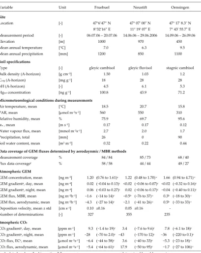
Table 1. Summary of site specifications, environmental conditions as well as atmospheric GEM and CO₂data.

Variable Unit Fruebuel Neustift Oensingen

Site Location [‐] 47°6’47” N 8°32’16” E 47° 07 00 N 11° 19 07 E 47° 17 8.3 N 7° 43 55.7 E Measurement period [‐] 06.07.06 – 20.07.06 14.06.06 – 29.06.2006 14.09.06 – 26.09.06 Elevation [m] 1000 970 450 Mean annual temperature [°C] 7.0 6.3 9.5 Mean annual precipitation [mm] 1200 850 1100 Soil specifications

Type [‐] gleyic cambisol gleyic fluvisol stagnic cambisol Bulk density (A‐horizon) [g cm−3_] _1.50 _1.03 _1.2 Corg (A‐horizon) [mg g−1_] ₁₈ ₂₈ ₂₈ pH (A‐horizon) [‐] 4.5 6.1 5.3 Hgtot concentration [ng g−1_] _100.8 _43.9 _71.2 Micrometeorological conditions during measurements Air temperature, mean [°C] 18.5 20.7 15.8 PAR, mean [μmol m−2_s−1_] ₅₆₀ ₅₅₀ ₃₁₀ Relative humidity, mean % 75.9 69.7 95.6 * u_, mean _[m s−1_] _0.17 _0.17 _0.12 Water vapour flux, mean [mmol m−2_s−1_] _2.7 _2.0 _1.7 Precipitation, total [mm] 26 0 90 Soil water content, mean [m3 m−3_] _0.32 _0.22 _0.44 Data coverage of GEM fluxes determined by aerodaynmic / MBR methods Measurement coverage % 84 / 84 85 / 73 68 / 40 Flux data coveragef % 58 / 58 44 / 44 49 / 27 Atmospheric GEM

GEM concentration, mean [ng m−3_] _{1.20 (0.76 to 1.61)}c 1.22 (0.48 to 1.70) c _{1.66 (0.94 to 4.71)} c GEM gradienta_{, day, mean} _[ng m−4_] _{0.02 (−0.04 to 0.13)}c _{<0.02 (−0.06 to 0.07)}c_{<0.02 (−0.32 to 0.16)}c GEM gradienta, night, mean [ng m−4_] _{0.06 (−0.03 to 0.27)}c 0.02 (−0.06 to 0.17)c −0.04 (−0.40 to 0.11)c GEM flux, MBR, mean [ng m−2_h−1_] _{−1.6 (−14 to 14)}c _−0.5b_{(−76 to 37)} c _0.3b_{(−18 to 30)} c GEM flux, aerodynamic, mean [ng m−2_h−1_] _{−4.3 (−27 to 14)}c −2.1 (−41 to 26) c _0.5b (−33 to 33) c Deposition velocity, mean ± std [cm s−1_] _{0.10 ±0.16} _{0.05 ±0.16} _‐ Number of determinations [‐] 327 355 235

Atmospheric CO2

CO2 gradienta_{, day, mean} _[ppm m−1_] _{9.3 (−1.4 to 19)}c _3.4 _{(−7.6 to 9.6)}c _{7.8 (−6.1 to 18)}c CO2 gradienta, night, mean [ppm m−1_] ₋₂₈ _{(−70 to 2.0)}c −43 (−170 to 12)c −36 (−220 to 0.1)c CO2 flux, ECe_, mean _[μmol m−2_s−1_] _{−6.4 (−44 to 58)}c _3.6 _{(−40 to 33)}c _{−5.3 (−23 to 18)} c CO2 flux, aerodynamic, mean [μmol m−2_s−1_] _{−5.4 (−64 to 61)}c 17.9 (−50 to 95)c −1.7 (−27 to 106) c a calculated as described in section 2.5 not significantly different from zero c range standard error e determined by eddy covariance minimum resolvable gradient as mean +1 std

(25)

ACPD

Full Screen / Esc

EGU Table 2. Correlation of GEM concentration with meteorological variables.

Variable Fruebuelb _Neustiftc _Oensingend

r p r p r p Air temperature −0.39 < 0.05 −0.77 < 0.05 −0.30 < 0.05 Soil temperature −0.28 < 0.05 −0.64 < 0.05 −0.26 < 0.05 PAR −0.17 < 0.05 −0.56 < 0.05 −0.27 < 0.05 Soil water content 0.44 < 0.05 0.31 < 0.05 −0.30 < 0.05 Absolute humidity 0.44 < 0.05 0.65 < 0.05 −0.08 0.14 Relative humidity 0.66 < 0.05 0.82 < 0.05 0.47 < 0.05 CO2 concentration (LI‐6262) 0.11 < 0.05 0.31 < 0.05 0.66 < 0.05 CO2 flux (eddy covariance) 0.21 < 0.05 0.09 0.15 −0.03 0.81 H2O flux (eddy covariance) −0.16 < 0.05 −0.61 < 0.05 −0.52 < 0.05 O3 concentrationa −0.43 < 0.05 ‐ ‐ −0.54 < 0.05 Wind speed 0.05 0.35 −0.52 < 0.05 −0.33 < 0.05 adata from nearest national monitoring station; bN=255 – 390; cN=194 – 375; dN=31 – 337

(26)

ACPD

Full Screen / Esc

Printer-friendly Version Interactive Discussion G E Ma ir [n g m -3] 0.0 0.4 0.8 1.2 1.6 Tair [°C ] 10 15 20 25 30 35 P AR [µ m o l m -2s -1] 0 500 1000 1500 2000 time [days] 0 1 2 3 4 5 6 7 8 9 10 11 12 13 14 C O2 fl u x [µ m o l m -2s -1] -30 -10 10 30 50 G E Mg ra d ie n t [n g m -4] -0.1 0.0 0.1 0.2 R H [% ] 0 20 40 60 80 100 u* [m s -1] 0.0 0.2 0.4 0.6

thin: aerodynamic method bold: EC C O2 g ra d ie n t [p p m m -1] -60 -40 -20 0 20

dotted: relative humidity

G E Mfl u x [n g m -2h -1] -15 -10 -5 0 5 G E M flu x [n g m -2h -1] -15 -10 -5 0 5 aerodynamic method shaded: standard deviation

MBR method shaded: standard deviation dotted: PAR

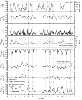
Fig. 1. Time series of measurements at Fruebuel. From top to bottom: air temperature (T_air), photosynthetically active radiation (PAR), atmospheric GEM concentration at 1.7 m above ground (GEM_air), friction velocity (u_∗), GEM gradients and relative humidity, CO₂gradients, tur-bulent fluxes of GEM (determined by the aerodynamic and MBR methods) and CO₂ (deter-mined by the aerodynamic method and the eddy covariance technique). Flux data and GEM gradients were filtered by a 9-point moving average. Positive fluxes indicate emission, negative deposition.

(27)

ACPD

Full Screen / Esc

Printer-friendly Version Interactive Discussion EGU G E Mfl u x [n g m -2h -1] -10 -5 0 5 10 15 G E Ma ir [n g m -3] 0.0 0.4 0.8 1.2 1.6 Tair [°C ] 10 15 20 25 30 35 P AR [µ m o l m -2s -1] 0 500 1000 1500 2000 time [days] 0 1 2 3 4 5 6 7 8 9 10 11 12 13 14 15 16 C O2 fl u x [µ m o l m -2s -1] -20 0 20 40 60 80 G E Mg ra d ie n t [n g m -4] -0.1 0.0 0.1 0.2 R H [% ] 0 20 40 60 80 100 u* [m s -1] 0.0 0.2 0.4 0.6

thin: aerodynamic method bold: EC C O2 g ra d ie n t [p p m m -1] -180 -140 -100 -60 -20

dotted: relative humidity

G E Mfl u x [n g m -2h -1] -10 -5 0 5 10 15 aerodynamic method shaded: standard deviation

MBR method shaded: standard deviation

dotted: PAR

(28)

ACPD

Full Screen / Esc

Printer-friendly Version Interactive Discussion G E Mfl u x [n g m -2h -1] -5 0 5 10 15 G E Ma ir [n g m -3] 0 1 2 3 4 Tair [°C ] 10 15 20 25 30 35 P AR [µ m o l m -2s -1] 0 500 1000 1500 2000 time [days] 0 1 2 3 4 5 6 7 8 9 10 11 12 13 C O2 fl u x [µ m o l m -2s -1] -20 0 20 40 60 G E Mg ra d ie n t [n g m -4] -0.2 -0.1 0.0 0.1 0.2 S W C [ % -v o l] 38 42 46 50 u* [m s -1] 0.0 0.2 0.4 0.6

thin: aerodynamic method bold: EC C O2 g ra d ie n t [p p m m -1] -350 -250 -150 -50 50

dotted: soil water content

G E Mfl u x [n g m -2h -1] -5 0 5 10 15 aerodynamic method shaded: standard deviation

MBR method shaded: standard deviation

dotted: PAR

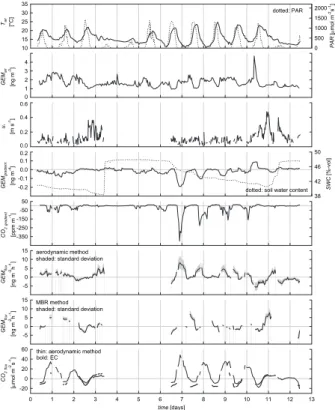
Fig. 3. Same as Fig.1, but study site Oensingen. Soil water content is shown instead of relative humidity in panel four.

(29)

ACPD

Full Screen / Esc

Printer-friendly Version Interactive Discussion EGU hour of day 11 13 15 17 19 21 23 G E Ma ir [ n g m -3 ] 0.6 0.8 1.0 1.2 1.4 1.6 1.8 2.0 2.2 2.4 Oensingen Fruebuel Neustift 1 3 5 7 9

Fig. 4. Diurnal trend of atmospheric GEM concentrations at the three study sites. Shown are hourly mean and standard errors of all measurement days (Fruebuel 14 days, Neustift 16 days, Oensingen 11 days).

(30)

ACPD

Full Screen / Esc

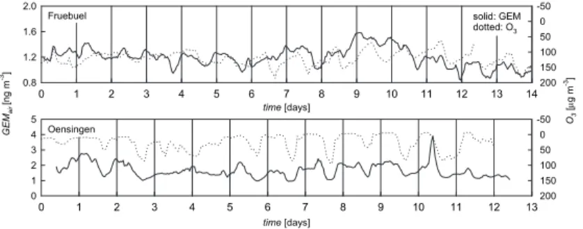
Printer-friendly Version Interactive Discussion time [days] 0 1 2 3 4 5 6 7 8 9 10 11 12 13 14 G E Ma ir [n g m -3] 0.8 1.2 1.6 2.0 O3 [µ g m -3] -50 0 50 100 150 200 Fruebuel time [days] 0 1 2 3 4 5 6 7 8 9 10 11 12 13 0 1 2 3 4 5 -50 0 50 100 150 200 solid: GEM dotted: O3 Oensingen

Fig. 5. Time series of atmospheric GEM and ozone concentrations (O₃) at Fruebuel and Oensingen. GEM concentrations were filtered by a 3-point moving average. Oneµ g m−3

of O₃ corresponds to 0.5 ppb.