Comparison between modelling and measurement of marine dispersion, environmental half-time and 137Cs inventories after the Fukushima Daiichi accident

HAL Id: hal-02433219

https://hal-normandie-univ.archives-ouvertes.fr/hal-02433219

Submitted on 14 Jan 2020

HAL is a multi-disciplinary open access

archive for the deposit and dissemination of

sci-entific research documents, whether they are

pub-lished or not. The documents may come from

teaching and research institutions in France or

abroad, or from public or private research centers.

L’archive ouverte pluridisciplinaire HAL, est

destinée au dépôt et à la diffusion de documents

scientifiques de niveau recherche, publiés ou non,

émanant des établissements d’enseignement et de

recherche français ou étrangers, des laboratoires

publics ou privés.

Comparison between modelling and measurement of

marine dispersion, environmental half-time and 137Cs

inventories after the Fukushima Daiichi accident

Pascal Bailly Du Bois, Pierre Garreau, Philippe Laguionie, Irène Korsakissok

To cite this version:

Pascal Bailly Du Bois, Pierre Garreau, Philippe Laguionie, Irène Korsakissok. Comparison between

modelling and measurement of marine dispersion, environmental half-time and 137Cs inventories

af-ter the Fukushima Daiichi accident. Ocean Dynamics, Springer Verlag, 2014, 64 (3), pp.361-383.

�10.1007/s10236-013-0682-5�. �hal-02433219�

Comparison between modelling and measurement of

marine dispersion, environmental half-time and 137Cs

inventories after the Fukushima Daiichi accident.

P. Bailly du Bois1✉ <Email: pascal.bailly-du-bois@irsn.fr> P. Garreau2

P. Laguionie1 I. Korsakissok3.

[1] Institut de Radioprotection et de Sûreté Nucléaire (IRSN), PRP-ENV/SERIS/LRC Cherbourg-Octeville, France [2] Institut Français de Recherches et d'Etudes sur la Mer (IFREMER), DYNECO, Brest, France

[3] Institut de Radioprotection et de Sûreté Nucléaire (IRSN), PRP-SESUC/BMTA, Fontenay-aux-Roses France

Abstract

Contamination of the marine environment following the accident at the Fukushima Daiichi nuclear power plant (FDNPP) represents the most important influx of artificial radioactivity released into the sea ever recorded. The evaluation, in near real time, of the total amount of radionuclide released at sea and of the residence time in coastal waters were ones of challenges for nuclear authorities during this event. In the framework of a crisis situation, a numerical hydrodynamical model has been built and used 'as is'. The concomitant use of this numerical model and in situ data allows the comparison of the simulated and measured environmental half-times. A tuning of the wind drag coefficient has been nevertheless necessary to reproduce the evolution of measured inventories of 137Cs and 134Cs between April and June 2011. After tuning, the relative mean absolute error between measured and simulated concentrations for the 849 measurements in the dataset is 69 %, while the relative bias indicates a model underestimation of 4%. These results confirm the estimates of the source term, i.e. 27 PBq (12 - 41 PBq) for direct releases and 3 PBq for atmospheric deposition onto the sea. The parameters applied here to simulate atmospheric deposition onto the sea are within the correct order of magnitude for reproducing seawater concentrations.

Quantitative inventories of tracers which integrate dispersion and transport processes are useful to test model reliability. It exhausts the model sensibility to meteorological forcing, which remains difficult to appraise to reproduce mid- to long-term transport.

Keywords

Fukushima accident; Caesium 137; coastal modelling; environmental half-time; radionuclide; Pacific Ocean

Ocean Dynamics, accepted 12/2013

Communicated By

Responsible Editor: Martin Verlaan Misc

This article is part of the Topical Collection on the 2012 16th biennial workshop of the Joint Numerical Sea

1 Introduction

Contamination of the marine environment following the accident at the Fukushima Daiichi nuclear power plant (FDNPP) occurred (1) after dry and wet deposition from a contaminated atmospheric plume directed mainly offshore between March 12 and March 23; (2) from direct releases of highly contaminated waters into the sea, which were clearly identified from the end of April; and (3) from the transport of radioactive pollution due to leaching of contaminated soil after atmospheric deposition on Honshu island.

The direct liquid releases from FDNPP represent the largest influx of artificial radioactivity into the sea ever occurring over a short period of time on a small spatial scale (Aarkrog 2003; Linsley et al. 2005; Livingston and Povinec 2000; Buesseler et al. 2011). Although controlled releases of liquid effluent from the Sellafield reprocessing plant can be compared in terms of total quantities, they have occurred over several years (1970-1980) instead of days, weeks and months as in the case of the FDNPP accident (Bailly du Bois et al. 2012b).137Cs inputs to the atmosphere and seawater have been estimated by different authors (Bailly du Bois et al. 2012b; Chino et al. 2011; Honda et al. 2012; Kawamura et al. 2011a; Morino et al. 2012; NERH 2011; Stohl et al. 2011; Tsumune et al. 2012; Yasunari et al. 2011; Schöppner et al. 2012; Korsakissok et al. 2013) Table 1 summarizes the methods applied by these authors and the results obtained. The 137Cs total atmospheric source term varies from 10 to 36 PBq, (Schöppner et al. 2012) implies a much higher activity (1,000 – 10,000 PBq) in the total inventory of radionuclides released. Fewer estimates have been made of atmospheric deposition onto the sea, which is much more difficult to assess compared with land deposition because data are not available immediately after deposition and water masses move and dilute the seawater plume before measurements can be carried out. This explains why the parameters describing deposition onto the sea are difficult to validate.

Table 1. Marine source term estimations after the FDNPP post tsunami disaster of 2011, according to the various recent studies.

Atmospheric release Direct release

Sea surface deposit

Source Evaluation method 137_{Cs (PBq)} 131_I/137_Cs* Total137Cs (PBq) 137Cs (PBq) (area in km) 131_I/137_Cs* (Bailly du Bois et al. 2012b) 137

Cs inventory and environmental half time deduced from measurement

+ pX model for atmospheric release

27

(12 - 41) 20 11.5

0.076

(50x100) 14 (Chino et al. 2011) SPEEDI model/measurements

comparison 13 (2.6 - 65) 11.5 (Honda et al. 2012) AQF model 15 0.18 (2700x3500) (Kawamura et al. 2011b)

Initial dilution of TEPCO flux in a 1.5 x 1.5 km x 1m area, SEA-GEARN model/measurement comparison 4 2.8 13 5 (1700x2100) 11.4 (Mathieu et al. 2012) pX model 20 (Morino et al. 2012) model/measurement comparison CMAQ 9.94 1 (700x700) 27 (NERH 2011)

Leakage evaluation from video observations of a 30 mm outflow

during 1-6 April

0.94 19,9 15

(Schöppner et al.

2012) ATM model/measurement comparison

1000 – 10 000

(Stohl et al. 2011) FLEXPART model with inversion algorithm from measurements

35.8

(23.3-50.1) 28 (78% of total) (Tsumune et al.

2012)

Initial dilution of TEPCO flux in a 1 x 1 km area, model/measurement

comparison (ROMS)

3.5

(2.8 – 4.2)

Lower than direct release (Yasunari et al. 2011) FLEXPART model/measurement comparison 12 1 (1700x1700) This work, (Korsakissok et al. 2013) pX model updated 20 3 (80x80)

Estimation of the inventories of radionuclides introduced in the marine environment is a crucial issue for assessing their impact and thus governs future studies on the behaviour of contaminated waters and radioactivity transfers to living species and sediments.

Mid- to long-term conservative tracer measurements are powerful tools for checking the dilution and renewal times of marine dispersion models. Radionuclides are useful in this context, and they have been extensively applied on the European continental shelf by using controlled liquid releases from reprocessing plants at Sellafield and La Hague (Salomon et al. 1995; Breton and Salomon 1995; Guéguéniat et al. 1993; Kershaw et al. 1999; Bailly du Bois et al. 1995; Bailly du Bois et al. 2012a; Shonfëld 1995; Kautsky 1988). Numerous samples and measurements obtained after the FDNPP accident provide the opportunity to perform comparable studies.

An estimation of the total direct release was performed by calculating the inventory of 137Cs derived from time evolution of interpolated surface seawater measurements. The blue box on Fig. 1 shows the area within which measurements were interpolated, i.e. latitude 36.93°-37.82° N; longitude: 140.9°-141.45 W° (100 km x 50 km). Details of the method and assumptions applied are presented in (Bailly du Bois et al. 2012b). The choice of this area is based on availability of sufficient numbered data to calculate inventories during the months following the FDNPP accident (126– 395 individual measurements for each calculation). The main uncertainty of the method stems from the evaluation of the mixing layer thickness inferred from hydrographic measurements. A map representing the spatial variation of this thickness was used for the calculation of137Cs inventories; the average depth of the mixing layer is 32 m. The error associated with this quantification is estimated to be ca. 50%.

(a) (b)

Figure 1. (a) Map showing extent of the model domain. The blue box delimits the area covered by the137Cs inventory. (b) Modelled sea surface current (April 2011 mean current).

The evaluation of direct release performed by (Bailly du Bois et al. 2012b) is based on inventories calculated from measurements performed at sea by Japanese organizations. These inventories show a short environmental half-time of 6.9 days in the 50 x 100 km area offshore from the FDNPP (Fig. 1 a, Fig. 2). This environmental half-time represents the time in which one half of the radioactivity is removed from the calculation area.

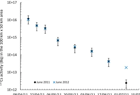
1E+12 1E+13 1E+14 1E+15 1E+16 1E+17 08/04/11 22/04/11 06/05/11 20/05/11 03/06/11 17/06/11 01/07/11 15/07/11 13 7Cs ac tiv ity (B q) in th e 10 0 km x 50 km ar ea June 2011 June 2012

Figure 2. Time evolution of 137Cs activity in a 50 x 100 km area around the FDNPP, calculated from data available in June 2011 (Bailly du Bois et al. 2012b) and in June 2012.

The present study investigates the capacity of a hydrodynamic dispersion model to asses this environmental half-time and tests the main assumption applied in the calculation of inventories: the mixing layer thickness. The order of magnitude of the atmospheric deposition is investigated by model versus measurement comparisons. Global and daily models are also compared with measurements obtained from individual seawater samples.

This paper also defines the different sources of 137Cs that are taken into account in the model vs. measurement comparison: direct releases from the FDNPP, atmospheric deposition and water runoff on catchment areas. The Ifremer-MARS3D hydrodynamic model applied in this study is also described. We use the data available in the framework of a crisis situation. It accounts for main forcing governing advection and diffusion in the concerned area. It concerns mainly the regional and local circulation, wind forcing and tides. The model tuning is based on comparison with 137Cs measurements obtained in seawater between march and June 2011, i.e.: direct release estimation (Bailly du Bois et al. 2012b) and measured inventories between April and June 2011.137Cs is modelled as a passive tracer that advects and diffuses into the seawater. The amount of137Cs decreases by radioactive decay according to a half-life of 30 years. This decay effect is negligible during the simulation period of a few months used in this study.

We test different tuning parameters, i.e. fluid viscosity, tide, horizontal diffusion coefficient and wind drag coefficient. As observed in previous studies (Bailly du Bois and Dumas 2005), this latter parameter appears sensitive for simulation of mid- to long-term dispersion of dissolved substances in marine systems.

The main purpose of the present study is to give tools to compare and refine the renewal times of models, by carrying out a quantitative comparison of measured and simulated tracers.

The modelled and measured half-times are discussed. Then, comparisons are carried out involving mixing layer thickness, as well as individual concentrations resulting from atmospheric deposition and direct releases. The discussion highlights the strengths and limits of the model tuning and the source term estimates.

2 Methods

2.1 137Cs seawater measurements

The seawater measurements reported here come from a compilation of monitoring data (Laguionie et al. 2012) provided on the Internet by TEPCO (TEPCO 2011), Ministry of Education, Culture, Sports, Science and Technology (MEXT) (MEXT 2011), Fukushima Prefecture, Hokkaido University and already published results (Inoue et al. 2012; Buesseler et al. 2012; Honda et al. 2012; Aoyama et al. 2012; Caffrey et al. 2012). The database includes 948 significant measurements of137Cs activity in seawater (above the detection limit, which varies with time) carried until to 20 July 2011 and the results from more than 7000 seawater samples analysed until May 2012. This database is provided as a supplementary material (A).

Caesium-137 activity concentrations in seawater off the eastern coast of Japan prior to the accident were of the same order of magnitude as other surface oceanic waters, yielding values of between 0.001 and 0.003 Bq.L-1(Nakanishi et al. 2011). After the accident, measured activity concentrations within a 30 km radius around the plant exceeded 10 Bq.L-1 and reached 68 000 Bq.L-1close to the plant.

The radionuclides with short radioactive half-life (less than a few tens of days, such as131I) ceased to be detectable after a few months and thus should not have any long-term impact. Other radionuclides, such as134Cs,106Ru and90Sr, will persist in seawater for several years. The persistence of these radionuclides in the water column is dependent on their respective affinities for the suspended particles in surface waters, which are likely to settle out and carry the radionuclides to the seabed.

Caesium-137 is readily soluble in seawater and could be advected over long distances by marine currents and dispersed throughout the Pacific Ocean water masses (Aoyama and Hirose 2003; Livingston and Povinec 2000; Povinec et al. 2004; Sanchez-Cabeza et al. 2011; Prants et al. 2011). A fraction of the caesium and other radionuclides will bind to suspended particles and cause sedimentary contamination by deposition on the seafloor, as observed previously with atmospheric fallout from nuclear tests (Lee et al. 2005; Moon et al. 2003) or controlled industrial releases (Bailly du Bois and Guéguéniat 1999). These latter authors show that the137Cs loss from seawater represents less than 20% of the quantities released after 6-months dispersion in the English Channel. This sea is characterized by strong tidal currents and shallow waters (less than 50 meters), which result in high SPM concentrations. In the North Pacific Ocean off Fukushima, half-time of137Cs in surface water has been estimated to 12±1 years (Povinec et al. 2005). For durations of months and scales of ten kilometers off the coast considered here, dissolved 137Cs could be considered as mainly conservative. The concentrations of this radionuclide are globally representative of other soluble radionuclides introduced into the sea over periods of months. Although different origins of the pollution could result in variable ratios of137Cs to other radionuclides in the source terms,137Cs fluxes give a good estimate of other radionuclides released at the same time. Results presented here are based on measurement in seawater without estimation of 137Cs fixed in suspended matter (SPM). Accounting for a SPM concentration of 10 mg.L-1and a Kd of 4000 (IAEA 2004), 4 % of Cs would be fixed on SPM. SPM concentrations are generally lower in open ocean waters, and measurement errors are 8% in average between March and July 2011. It concludes that filtering seawater or not would give no significant differences in monitoring measurements. Nevertheless, radionuclides fixed on SPM and deposed on the seabed are potential source terms for benthic living species concerned by transfer through SPM coming from deposited sediments, rivers or desorption in seawater of radionuclides fixed onto sediments. Such processes have been clearly identified in the Irish Sea after Sellafield releases (Jones et al. 2007; Finegan et al. 2009). Storm events could also remobilize significant quantities of137Cs and induce temporary higher concentrations in seawater.

To facilitate comparison between different types of labelling, all radionuclide/137Cs ratios are decay corrected to the initial ratio at the date of the tsunami of 11 March 2011, when the power plant ceased operating. This initial ratio is referred to here as IR (radionuclide/137Cs).

As the input of caesium occurs via surface waters, it mixes into a 20-50-m thick surface layer near the coast. This layer can reach a thickness of 100 m further offshore. Hydrographic measurements of temperature and salinity performed by JAMSTEC – MERI (Marine Ecology Research Institute) around the site between 28 March and 3 May 2011 yield a better estimate of this mixing close to the FDNPP. Dispersion of the soluble fraction of the radionuclides will mainly take place in the surface mixing layer. In addition, the fraction of radionuclides associated with solid particles could be transported to the seabed by sedimentation (Lee et al. 2005; Moon et al. 2003; McCartney et al. 1994; Povinec et al. 2005).

2.2 Direct releases from FDNPP and environmental half time

The high concentrations recorded in the seawater in the immediate vicinity of the FDNPP indicate that one or more sources of radioactive liquid effluent escaped directly from the nuclear power plant. These sources of effluent correspond to the water used to cool the damaged reactors. It has been confirmed that part of the water present in the damaged reactors (in particular, reactor No. 2, where the bottom part was damaged) leaked from the containment building and subsequently flowed out into the sea (NERH 2011).

Fig. 2 shows the time evolution of137Cs inventories, reporting the initial values compiled from the results available in July 2011 (Bailly du Bois et al. 2012b), along with an update including the results available in June 2012. Except in

July, there are only very slight relative differences with the new dataset, even if far more analyses have become available (Table 2). In July 2011, most of the available results were below the detection limit (lower than 10 Bq.L-1). The values obtained during the following months were more precise, which leads to a more representative map of the labelling. The same calculation was performed with currently available 134Cs measurements, showing very similar results (Fig. 7), since the value of IR (radionuclide/137Cs) is close to 1 and the 134Cs environmental half-time of two years is not perceptible at this time scale.

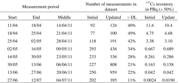
Table 2.137Cs inventories calculated from interpolation of individual measurements in seawater in a 100 x 50 km box off Fukushima Daiichi plant (blue box on Fig.1); initial values based on data available in June 2011, and

updated with data available in June 2012.

Measurement period Number of measurements in dataset

137_{Cs inventory}

in PBq (± 50%) Start End Middle Initial Updated > DL Initial Update

11/04 18/04 14/04/11 92 126 40% 11.6 10.4 18/04 25/04 21/04/11 77 100 49% 4.75 4.68 25/04 02/05 28/04/11 118 191 42% 3.38 3.10 02/05 16/05 09/05/11 293 436 34% 0.667 0.689 16/05 30/05 23/05/11 233 336 28% 0.261 0.286 30/05 13/06 06/06/11 227 808 21% 0.163 0.158 13/06 27/06 20/06/11 250 959 22% 0.042 0.042 27/06 12/07 04/07/11 202 395 11% 0.0024 0.0190

The time evolution of activity follows an exponential power law, indicating an environmental half-time of 6.9 days in April and May 2011 (Bailly du Bois et al. 2012b). This environmental half-time represents the time in which one half of the137Cs activity is removed from the calculation area. This loss results from dilution by currents and inputs of non-contaminated water into the area considered for calculation. The regularity of this dilution is remarkable considering the variation of the circulation pattern observed in this area (JHOD 2011). This implies that whatever the detailed current direction at the time of the accident is, water mass fluxes were governed by the generally strong Kuroshio and Oyashio currents that are stable at this scale. This efficient dilution diminished the local impact of the accident in coastal waters: Contaminated waters will be transported rapidly to the east, into the central Pacific.

The observed dilution in the FDNPP area is based on hundreds of measurements integrated over space and time. We consider that this observed environmental half-time is a robust parameter for model comparison. If models provide an incorrect rate of water mass renewal, then all models versus measurement comparisons will be biased. Before any attempt can be made to compare measured and simulated concentrations of radionuclides, hydrodynamic models must first reproduce the average mixing and dilution observed in the studied area.

By extrapolating the regression curve at the date of 8 April 2011, while taking account of measurements close to the FDNPP for evaluation of inputs from April to July 2011, it is possible to calculate a total direct release of 27PBq as well as the time evolution of the137Cs flux from the plant (Bailly du Bois et al. 2012b). This source term has been used as input for the hydrodynamic model.

2.3 Atmospheric deposit onto the surface of the sea

Following the explosions and pressure venting of the reactor containments at the FDNPP, an atmospheric plume of contaminated aerosols was released, part of which was transported over the sea. The main atmospheric releases occurred between 12 March and 25 March. The subsequent plumes were dispersed over long distances: A homogeneous labelling of the Northern Hemisphere was simulated and measured after about 15 days (Masson et al. 2011; Mathieu et al. 2012). Part of the radionuclides contained in the atmospheric plume fell back to the sea surface by dry deposition or wet scavenging of the plume, leading to diffuse pollution of the surface water up to some tens of kilometers from the nuclear power plant. On the sea, it is difficult to assess this contamination because deposition covered a large area and was quickly advected and dispersed. To obtain an estimation of the amounts involved, we only have seawater measurements performed a few days after the release. Before March 24, when direct liquid release was still relatively

limited, the concentrations measured in seawater more than 10 km off the coast could be attributed to atmospheric deposition, with levels ranging from 9 to 13 Bq.L-1for137Cs and an IR(131I/137Cs) of 5 - 12. At the same time, another spike was observed along the coast at more than 10 km south of the plant, with137Cs activities in the range 20 - 100 Bq.L-1 and an IR(131I/137Cs) value of 35 - 110. This could be attributed either to atmospheric deposition or previous direct releases from the plant, or the influence of rivers after washout of contaminated soil by rain. These labelling results reveal at least two different kinds of sources for the radionuclide, possibly coming from different units within the plant (FDNPP units n°1, 2 or 3).

The total amount of 137Cs deposited on the sea surface was derived from atmospheric dispersion calculations using Institut de radioprotection et de sûreté nucléaire’s (IRSN) Gaussian puff model pX (Soulhac and Didier 2008). The model was forced with 3D meteorological forecasts at a resolution of 0.125° from the ECMWF (European Centre for Medium-Range Weather Forecast), provided by Météo-France (the French meteorological office). Rain radar observations were also used for a better estimation of precipitation location and timing. The atmospheric source term was estimated by IRSN, based not only on the reactor states but also on atmospheric gamma dose rate measurements both on-site and throughout Japan (Corbin and Denis 2012). This estimation remains highly uncertain, both in terms of released activity and timing. This is especially true for releases that were dispersed towards the open sea, where no atmospheric measurements are available. The deposition rates applied over seawater are lower than over land: a value of 5.10-5m.s-1was assumed for all particulate radionuclides (Pryor et al. 1999) and Maro D. (personal communication). Wet scavenging was modelled similarly over the sea and the land, with a scavenging coefficient expressed as Ap0B,

where A=5.10-5 hr.mm-1.s-1, B=1, and p0 is the rain intensity in mm.hr-1 (Sportisse 2007). Atmospheric simulation

results and comparisons with land-based measurements are presented in detail elsewhere (Mathieu et al. 2012; Korsakissok et al. 2013).

According to these simulations, the amount of atmospheric deposition on the sea surface calculated 80 km from FDNPP is 3 PBq with IR (131I/137Cs) = 14. This estimate is much higher than the value previously calculated in (Bailly du Bois et al. 2012b), which was based on an earlier source term estimation. Our simulation is based on a total atmospheric release of 20.6 PBq of137Cs. Thus, the 3PBq deposited on the sea surface corresponds to about 13% of the total amount of137Cs released, whereas 6% of this total was deposited on land at the same distance (80 km from the plant). Land measurements tend to confirm our estimates of total deposition, and simulations appear to be sufficiently robust (within a factor of 2) to changes in simulation parameters (Korsakissok et al. 2013).

Figure 3 presents the cumulated137Cs deposition onto the sea as calculated by pX. More than 99% of the atmospheric deposition over the sea comes from wet scavenging. In particular, the southern zone of deposition shown on Fig. 3 corresponds to releases occurring on 15-16 March, when heavy rains induced an intense plume wash-out both over the land and over the sea.

Figure 4 represents the time-evolution of atmospheric deposit and direct release accounted for simulation of dispersion. The main contribution of atmospheric deposit occurs on 15 – 16 March, twelve days before main direct release.

140.1 140.35 140.6 140.85 141.1 141.35 141.6 141.85 142.1 142.35 36.3 36.4 36.5 36.6 36.7 36.8 36.9 37 37.1 37.2 37.3 37.4 37.5 37.6 37.7 37.8 37.9 38 38.1 137

Cs deposition

Bq.m



Figure 3. Calculated cumulated atmospheric deposition of137Cs on 24 March 2011

Figure 4. Time evolution of the atmospheric deposit and the direct release of137Cs to the sea. 2.4 Water runoff on catchment areas

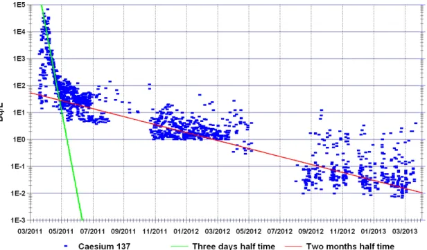
The radioactive terrestrial deposition resulting from the dispersion of atmospheric releases from the Fukushima Daiichi plant could be partially leached by rainwater and then transported to the sea by runoff. The contaminated land areas drained in this way could represent several thousands of square kilometers. Seawater measurements along the coast (see Fig 5) show that the rapid decline of mean 137Cs concentrations ceased after May 2011, corresponding to the rapid renewal of coastal waters (half-time of about three days along the coast, which does not correspond to the half-time

presented in Sect. 2.2 for an area of 100 x 50 km). This effect is counterbalanced by a much longer half-time of around two months from June 2011 to September 2012. This slow dilution reflects a continuous input of 137Cs into coastal waters. It could result from the drainage of catchment areas or sediment leaching. From the data available, we are not yet able to estimate which source is the most significant. After September 2012 we observe a stabilization of concentrations which probably reveals theses long-term influences and possibly some leakage from the plant area (Kanda 2013). Concentrations in March 2013 close to the plant were 0.3 Bq.L-1in average, around hundred times higher than concentrations occurring before the accident. Due to the uncertainties of these influences and their relative weakness at present, we do not take account of these source terms in the simulations covering the period from March to June 2011.

Figure 5. Time evolution of137Cs activity present in seawater at less than 10 km from the coast and less than 30 km from FDNPP, along with corresponding environmental half-times.

2.5 Numerical model configuration and results

The FDNPP is located on the east coast of Honshu island, 200 km northeast of Tokyo. The coast runs north-south, facing the Pacific Ocean. The water depth increases steadily offshore, reaching some 200 m at 50 km from the coast, increasing abruptly to 5000 m at distances of more than about 100 km offshore (Fig. 1).

In the zone most affected by radioactive pollution, the currents are generated by tides, the wind and the general circulation of Pacific water masses. On a short term basis, front of the outfall, the effect of the tide is predominant, leading to a back-and-forth motion of the water masses, with currents directed north and south along the coast at velocities of the order of 1 m.s-1 and a periodicity of 12 hours. The main part of the advection dispersion of radionuclides at regional scales is the consequences of the mesoscale structures in interaction with the wind and the global circulation.

The general large-scale circulation is the result of the interaction between the strong Kuroshio oceanic current, which comes from the south and runs along the coasts of Japan, and the Oyashio current, which comes from the north. The coastal waters in the vicinity of the Fukushima Daiichi plant are located in the convergence zone where these two currents interact, creating unsteady gyratory currents. These currents determine the medium-term dispersion of the radioactive pollution (from weeks to months). The long-term migration of the surface waters could be towards the south, but will not extend beyond the latitude of Tokyo. The Kuroshio current will act as a frontier and will carry the plume to the east towards the centre of the Pacific (Jayne et al. 2009).

We used the model for application at regional scale (MARS3D), (Lazure and Dumas 2008) to simulate the dispersion of

137

circulation model formulated using sigma coordinates. In this study, to remain applicable in a “crisis” situation, we use the MARS3D model 'as is'; this model is usually applied around the European continental shelf in both tidal and thermohaline context (Bailly du Bois et al. 2012a; Bailly du Bois and Dumas 2005; Batifoulier et al. 2012; Garreau et al. 2011). No specific adaptations were made for the FDNPP Pacific area, apart from the following details. The model domain covers the oceanic area off Fukushima: 31°N - 43.2°N, 137°E - 150°E (1000 km x 1200 km, Fig. 1 a). The horizontal resolution is around 1.852 km (one nautical mile, 1/60°) in both E-W and N-S directions, with 742 grid cells in the E-W direction and 622 in the N-S direction. The vertical resolution of the sigma coordinate is 40 layers refined near the surface. Bathymetric data are derived from JODC (JODC 2011).

The model accounts for the regional and local circulation, i.e. the Kuroshio current (high- density unstable current), the flux through the Tsugaru Strait, wind forcing (possibility of typhoons) and the tides (relatively weak, Fig 1b). It uses the data available in the framework of a crisis situation: The tide at open boundary conditions is prescribed using 16 tidal harmonic components from the FES2004 numerical atlas (Lyard et al. 2006)with a horizontal resolution of 1/8°. At the scale of thermohaline and geostrophic effects, the initial and boundary conditions are derived from the daily oceanic forecast and hindcast of the global model proposed by Mercator-Ocean with a resolution of 1/12° ( http://www.mercator-ocean.fr/eng (Ferry et al. 2007)). For the downscaling procedure, the temperature, salinity, currents and sea level are interpolated in both time and space to provide initial and boundary conditions.

Similarly, wind forcing, water and heat flux are downscaled from the atmospheric forecast and hindcast of the National Centers for Environmental Prediction (NCEP) meteorological global model (http://www.ncep.noaa.gov/) with a resolution of ½ degrees.

Using the Fukushima configuration described here, the parallelized MARS3D code runs on 256 MPI ranks.

During the crisis period, the model ran in the above described parameterization, hereafter called 'tide + initial wind' configuration. In a second approach, the wind drag coefficient has been tuned in order to fit the observed dispersion of radionuclides front of FDNPP (see discussion section 4.1). This modification of the atmospheric forcing led to an increase of the wind stress and is reported as 'wind stress increased' configuration. In a second time, different parameterizations with initial wind stress computation were also experienced to explore the model behaviour and were discussed below (figure 6 and figure 7). Among those, the fluid viscosity has been increased through the coefficient (from 0.05 to 0.25) in the Smagorinsky formulation for the horizontal diffusion of momentum (the 'increased viscosity' configuration). The role of the tide on the dispersion may be evaluated removing the external tidal forcing as tidal boundary conditions and tidal potential contribution in a 'no tide' configuration. The modification of the horizontal diffusion coefficient in the advection-dispersion of salt, heat and radionuclides did not exhibit any noticeable effect on the final results, indicating the importance of both global and mesoscale dynamics in contaminant transportation in this area. We perform also another simulation with the wind stress increased but with a time shift of two months (61 days) for the beginning of the release. This last simulation aims to test the effect of changes in the circulation between March and May in the dilution area. In all configurations the thermohaline forcing (Kuroshio-Oyashio convergence) has been taken into account as the main feature of this area.

The137Cs source term is derived from the calculated flux given in Fig. 6. in Bailly du Bois et al. 2012b. It represents the total inventory coming from direct releases, amounting to 27 PBq. The atmospheric deposition is calculated from the hourly deposition (see Sect. “Atmospheric deposit onto the surface of the sea”), with a total deposition onto the sea of 3PBq on 23 March 2011.

a) March 20-30, 2011

b) March 20-30, 2011

c) March 20-30, 2011

d) April 20-30, 2011

e) April 20-30, 2011

f) April 20-30, 2011

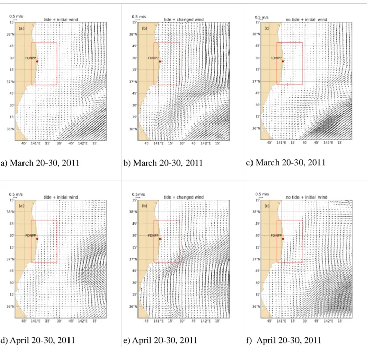
Figure 6. Time averaged of tidally filtered surface current simulated near FDNPP for end of March (a, b, c) and end of April (d, e, f). The model is running « as is » (a, d), using an increased drag coefficient_Cd _{x W}

0.8

0015 . 0

 (b, e) and « as is » without any tidal forcing (c, f). Red frame represents the inventory area.

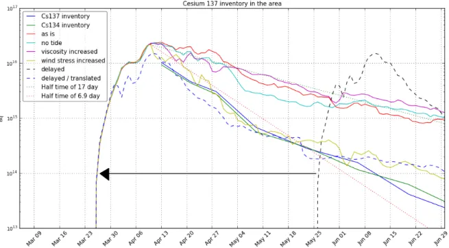
Figure 7. Time evolution of measured and simulated137Cs inventories present in the calculation area, as well as measured134Cs inventory.

3 Results

3.1 Sensitivity tests

Numerous models have been performed in this context of Fukushima accident, and comparisons are under process or have been already published. Masumoto et al. (2012) asses 6 different numerical models comparing the 10 days time-averaged surface circulation for the last days of March and April. Results for three different configurations of our model are presented in Fig. 6. Figure 6 a, d) corresponding to three of the above described configurations. In a second configuration (figure 6 – b, e) the wind forcing has been modified (increased) to fit the measured dispersion of dissolved radionuclides (see below). The last configuration deals with the removal of the tidal motion from the boundary condition. In March, all models (Fig. 2 of Masumoto et al. (2012)) exhibit a strong northeastward or eastward current – the Kuroshio - in the southeastern corner of the common domain and a southward current stopped by the Kuroshio front of Ibaraki (36°30' N). The current intensity in the Kuroshio can reach 1 m/s and the Southward current is weaker (0.2 - 0.5 m/s) The residual Eulerian circulation near the coast in front of the FDNPP is less evident, and very weak southward current is also computed in our simulations. Taking into account, the tides do not change drastically the surface circulation. An increase of the wind forcing through the modification of the drag coefficient acts on the surface mean current, generating a stronger southward current front of the FDNPP. In April (Fig. 6 d, e, f), the Kuroshio current moves northwards and meanders offshore until 37°N. A secondary weaker branch flows along the coast and could carry radionuclides northwards in front of the release position. This pattern is present for some models in the ensemble examined by (Masumoto et al. 2012). The differences between the simulated dynamics with (Fig. 6 d) and without tide (Fig. 6 f) suggest the importance of the mesoscale processes in this area. Adding the tide modifies the position of structures in April. One could expect that a relatively slight modification in model forcing or parameterization may have a strong incidence on the small-scale shelf circulation. The Kuroshio is a permanent and meandering current transporting offshore the contaminants, but the Fukushima outfall is not directly connected to this oceanic conveyor. The cross shelf exchanges are probably dominated by short-term living structure like eddies, coastal jet strongly depending on a 'chaotic' thermohaline circulation in that convergence area.

3.2 Comparison of measured and simulated environmental half time and137Cs inventories

The first issue in assessing the model’s reliability is to match the observed environmental half-time, which reflects the general circulation and dilution of water masses. The data presented in Sect. 2.2 allow us to perform this evaluation by comparing the time-evolution of137Cs inventories present in the FDNPP area from March to July 2011. The model simulates the amounts of137Cs present in the same area and over the same period as the available measurements. The

results are presented in Fig. 7, which reports the updated measured quantities as discussed in Sect. 2.2 (black line). The initially calculated simulated inventories are represented as a red line. The graph shows different trends of variation between measured and simulated inventories: The environmental half-time derived from simulation is around 17 days (light red line), instead of 6.9 days obtained from measurements between 8 April and 9 May (light blue line). While the initial inventories inferred for 8 April are similar, except with wind stress increased, the discrepancies increase with time for all simulations to reach a factor of more than ten after May 2011. This indicates that the model underestimates the rate of transport and dilution of water masses in the considered area.

This result is not surprising, as we have observed similar differences in the English Channel and North Sea following studies of the dispersion of controlled releases from the AREVA-NC reprocessing plant at La Hague from 1988 to 1994 (Bailly du Bois and Dumas 2005). Quantitative comparisons between the model and measurements also show significant differences, with excessively slow mean renewal times obtained for model dispersion. At this stage of the study, we performed numerous tests (more than a thousand) to determine the best parameters which could fit the model with measurements. We found that the most sensitive parameters were the origin of the wind data (meteorological model) and the surface drag coefficient applied. For the period and area considered here, we use the ECMWF wind speed at 10 m and a surface wind drag coefficient Cdcalculated with a power factor p:

W

x

0015

.

0

C





W represents the wind vector module (Wx, Wy) at 10 m.

The power factor was set at 0.48. Using this value, the model fitted inventories evaluated from the 1 400 compiled measurements, with deviations of less than 5% and mean variations over English Channel and North Sea of 54% (r2=0.88).

The wind drag coefficient initially applied for the FDNPP area was a classically adopted value, with p=0 in Eq. (1), i.e. Cd= 0.0015. We set the value of p in order to fit with the measured time evolution of 137Cs amounts. The result is

shown as a light-green line in Fig. 7, with p=0.8 in Eq. (1). Of course, this formulation of the drag coefficient leads to an overestimation of the wind stress and may not be realistic in case of strong wind. As regard to the general circulation, this modification of the drag coefficients does not change the main patterns- position and strength of the Kuroshio current, generation of eddies and loops - but increases obviously the surface current variability.

The dilution rate in the model can also be changed by modifying the diffusion coefficient. This type of tuning was also tested, but it proved much less efficient than the surface wind drag coefficient to improve the fit with environmental half-time. In our calculation, the diffusion coefficient is fixed at 10 m2.s-1.

After adjustment of the drag coefficient, Fig. 7 shows a good agreement between measured and simulated amounts of

137

Cs in the inventory area. The model reproduces the environmental half-time of 6.9 days between April and May, and the inflexion of the half-time measured from May to July is also visible in the simulation results. This inflexion reflects a seasonal variation in meteorological forcing during this period, moving from a succession of gust to more calm weather conditions (except a gust in early June). The discrepancies in137Cs inventories are still significant in June. This could result from the underestimation of137Cs due to the high detection limits (10 Bq.L-1) for measurements performed during the months following the accident. The corresponding concentration was set to 0 instead of measured concentrations, and it could result in the underestimation of measured quantities in June. This effect is reduced in updated inventories calculated in July 2011 from 2011 to 2012 data (Fig. 2, Table 2).

Figure 7 reports also the results with no tidal forcing and, as a sensitivity test, with viscosity increased (pink line) and with a time shift of two months (61 days) for the direct release. This time shift was applied to investigate the possible influence of particular dispersion conditions following the FDNPP accident that could explain the observed concentrations (wind and open boundaries conditions). For this last test, the black dashed line represents the evolution of the inventory at the date of the simulation. The blue dashed line represents the same values with a time translation at the date of the real release in March for comparison of the dilution. These results are discussed in section 4.1

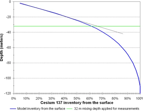
3.3 Mixing layer thickness

The main uncertainty in calculating 137Cs inventories from seawater measurements concerns the estimation of the mixing layer thickness. This value could be extracted from model results by horizontal integration of the amounts of

137_{Cs present over the calculation area as a function of depth. The result of this calculation is presented in Fig. 8 (blue}

line). The inventory calculated from the surface results in 65% of137Cs present between 0 and 32 m (green line) and 80% between 0 and 50 m depth from surface. The straight black line shows that the evolution in137Cs inventories is nearly linear from the surface down to 30 m depth. This proportionality between depth and quantities reveals efficient mixing and homogenization in this surface layer. It confirms the order of magnitude of the average mixing layer depth accounted for by the 137Cs inventory from surface measurements (green line in Fig. 8). This value (30 m) is also in agreement with rough estimates of the surface Ekman layer at this latitude. Nevertheless two strong down-welling favourable gusts occur (April 18th, May 29th) pushing coastal contaminated water under the surface mixing layer. As a result the extrapolation of the contamination in the surface layer could induce an underestimation of the total amounts of137Cs deduced from surface measurements.

Figure 8.137Cs inventory present over the calculation area vs. depth of surface layer.

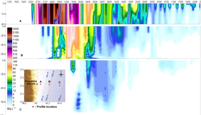
Figure 9 presents the time evolution of137Cs concentrations from direct release (a) and atmospheric deposit (b), at three points located east of Fukushima Daiichi. It shows an efficient mixing up to 50 m depth from March to May and confirms the assessment from (Masumoto et al. 2012): 'during March and April, several low-pressure systems passed through the Fukushima region, and they could have produced relatively large vertical mixing in this region'. Stratification occurs in May and for the profile located at 120 meters depth. Figure 9a shows variations of concentrations with time, which result mainly from wind variations combined with location of labelled water masses around of the different points (A, B, C).

Figure 9a. Time evolution of vertical concentrations of137Cs from direct releases at three locations, east of Fukushima Daiichi

Figure 9b. Time evolution of vertical concentrations of137Cs from atmospheric deposit at two locations, east of Fukushima Daiichi

3.4 Atmospheric deposit

It is difficult to assess the model’s ability to reproduce measurements associated with atmospheric deposition because measurements at sea are few in number and the source of the labelling is not clear when samples are collected close to the shore, near the FDNPP or after the beginning of direct releases. Nevertheless, it is still interesting to adopt an order of magnitude approach since there are large uncertainties concerning the area of wet deposition and the parameters applied.

Figure 10 presents a comparison between measured and simulated concentrations of137Cs at more than 2 km from the FDNPP before April 1, when direct releases were not the main origin of seawater labelling (Fig. 4). This figure shows that simulations give an order of magnitude of concentrations in agreement with most of the measurements. However, the model underestimates concentrations over a significant part of the studied domain, particularly at 30 – 60 km from the FDNPP. There is also an overestimation by the model for 26-27 March at 11-20 km from the plant. This model versus data comparison represents a broad confirmation of the deposition parameters applied at this scale. Figure 11 shows maps of measured and simulated concentrations from 23 to 28 March 2011, when most of measurements were available. It compares day by day the model outputs (background coloured plumes) with measurements (coloured dots in squares). On 23 and 24 March, significant labelling was measured at more than 20 km from the coast, which is not represented in the simulations. These discrepancies could stem from uncertainties in the wind direction, precipitation

and atmospheric releases (amount and timing). Besides, atmospheric releases after 17 March could not be attributed to particular events and were mainly fitted on land-based atmospheric measurements. Thus, atmospheric releases carried towards the sea at that time could have been overlooked. The complete results of this day-by-day comparison between simulations and measurements are presented as an appendix to this publication (Supplement B) Overall, the measured and simulated concentrations are of the same orders of magnitude.

1E-2

1E-1

1E0

1E1

1E2

1E3

S

im

u

la

te

d

c

o

n

c

e

n

tr

a

ti

o

n

,

B

q

/L

1E-2

1E-1

1E0

1E1

1E2

1E3

Measured concentration, Bq/L

Date, distance in km (N, S, E)

Figure 10. Measured versus simulated concentrations of137Cs for samples available between 21 and 31 March 2011 collected at more than 2 km from FDNPP (atmospheric deposition labelling).

Figure 11. Daily measured and simulated concentrations of137Cs from 23 to 28 March 2011, before the beginning of direct releases from FDNPP. Background plumes simulation; dots in coloured squares measurements. 3.5 Simulation of137Cs concentrations

Figure 12 shows a comparison between measured and simulated concentrations of137Cs from April 1 to June 30. On the whole, the concentrations correspond over the six orders of magnitude covered by the range of measured values. For the sake of clarity, dates and distances are reported only when deviations are greater than one order of magnitude. These deviations correspond mainly to values obtained at the beginning of April to the south of FDNPP. This possibly stems from the residual influence of atmospheric deposition, in an area where atmospheric deposition is not well simulated. If we exclude these data, the mean normalized gross error is calculated as follows:

For the 849 values compiled in the dataset, calculations were based on series of measured and computed concentrations at the same place and at the same date, using Eq (2).



Solving Eq (2) yields a mean normalized relative mean absolute error of 69%. If we do not apply Abs in Eq (2), we obtain the relative bias; this indicates that the model leads to a 4% underestimation of individual concentrations. This slight deviation is the consequence of the fitting of the simulated and measured quantities described in Sect. 3.1. The calculation of quantities used to fit the wind drag coefficient accounts for bathymetry at each location of measurement. So it is not surprising that the comparison accounting only for concentrations results in a slight bias.

1E-2

1E-1

1E0

1E1

1E2

1E3

1E4

1E5

S

m

u

la

te

d

c

o

n

c

e

n

tr

a

ti

o

n

,

B

q

/L

1E-2

1E-1

1E0

1E1

1E2

1E3

1E4

1E5

Measured concentration, Bq/L

13/6 86E13/6 86E13/6 86E13/6 86E13/6 86E13/6 86E13/6 86E 14/6 89N 14/6 90N 14/6 92N 14/6 38N 14/6 38N 14/6 38N 14/6 38N 15/6 38N 15/6 38N 16/6 134S 16/6 135S 16/6 134S 16/6 135S 16/6 135S 16/6 136S 16/6 137S16/6 138S16/6 138S 16/6 138S17/6 148S16/6 139S_{17/6 151S}17/6 143S17/6 146S 17/6 154S 17/6 158S 17/6 148S17/6 140S 24/6 1S 24/6 1N

Date, distance in km (N, S, E)

Figure 12. Measured versus simulated concentrations of137Cs for samples available between 1 April and 30 June. Dates and distances are reported when ratio is higher than 10.

Figures 13 and 14 show maps of measured and simulated concentrations from 14 March to 18 June 2011, when most of the measurements were available. These figures illustrate the good correspondence between measured and simulated concentrations. Nevertheless, some days show significant discrepancies between simulated and measured dispersion plumes (17, 19 and 30 April, 16-18 June).

Complete results of the daily simulation versus measurement comparison are presented in the supplementary materials as an appendix to this publication, reporting data on an intermediate (B) and far-field scale (C).

(c)

Figure 13 a - c. Measured and simulated concentrations of137Cs, on a daily basis from 14 April to 7 May, and for 15 May and 2 June 2011. Background plumes simulation; dots in coloured squares measurements.

(b)

Figure 14 a - b. Measured and simulated concentrations of137Cs from 7 to 18 June 2011, during the Ka'imikai-o-Kanaloa campaign (Buesseler et al. 2012). Background plumes simulation; dots in coloured squares measurements.

4 Discussion

4.1 Tuning of wind drag coefficient

We know that the wind drag coefficient is an important and sensitive parameter for simulation of the dispersion of dissolved substances in marine systems over periods ranging from weeks to years. The choice of source for the wind data can itself change the residual flux by a factor of two (Bailly du Bois and Dumas 2005). On the other hand, the friction effect of the wind on the sea surface is difficult to investigate. Coarse resolution atmospheric modelling (such as the NCEP configuration used here) underestimates strong wind situations and does not yield a precise simulation of gusts. Near the coast, the spatial (and temporal) variability of the wind stress is probably not well represented (there are only 2 cells of NCEP model in the box area). The adjustment proposed here involves a parameterization designed to enhance the wind effect. While improving the wind forcing is a good way to enhance model reliability, it is probably not an optimal representation of the hydrodynamics of the area. It could mask other weaknesses of the model or boundary conditions that are applied here. First, if a higher drag coefficient proves to be more representative of the real meteorological forcing, it would also be applicable to the global model encompassing the local MARS3D model (i.e. Mercator Ocean in this case). For each other case of meteorological or global model forcing, it would be necessary to fix a new drag coefficient.

The effects of others parameterizations (increased viscosity and tide removal) have less impacts on the 'dispersion law' in the considered volume (Figure 7) and the computed environmental half-time is similar in all simulation considering the initial wind. Despite the global slope remains about 6.9 days, detailed variation of the amount of137Cs in the coastal

box exhibits different behaviour. The tidal free simulation indicates a lower contaminant quantity in May, and the more viscous run shows a lower value during the second part of April. This relative 'unexpected' behaviour demonstrates the importance of the mesoscales processes for the dispersion, front of Fukushima. Perturbing slightly the parameterization or the dynamics of the model can modify the occurrence or the position of eddies, filaments or other chaotic patterns. In this context, a high temporal and spatial resolution for the wind forcing would be necessary in this area to better simulate (a least statistically) the mesoscale activity. Increasing the wind stress deduced from NCEP is a way to overcome the lack of temporal and spatial variability in both the atmosphere and the ocean.

The simulation with a time shift of the release shows very similar results, except a higher dilution rate during the first week after release at the end of May. The trends of the two curves are similar, with the same inflection after two months (in May for the release not delayed). This inflection could result of recirculation of labelled plumes that re-enters in the inventory area. After three months dilution is nearly the same. As mentioned in section 3.1, differences between measured and simulated quantities in June could result of underestimation of quantities due to high detection limits of

137

Cs and134Cs, less than 22% of measurements were significative during this period.

As pointed out in Sect. 2.5, we chose to apply an existing model 'as is' in order to reproduce rapidly the conditions of dispersion after the FDNPP accident. Other models with a better representation of local conditions (fresh water inputs, bathymetry, local winds, etc.) would more accurately simulate the mesoscale gyres in the area and the exact pathway of contaminated waters. The model comparison carried out by (Masumoto et al. 2012) reveals the variability between the different models applied. This author concludes that he 'cannot say that one model is better than another'. Nevertheless ,the results obtained show that, once this tuning is carried out, even a model not specially adapted for this type of marine area (open ocean, greater water depths and mixing of strong geostrophic currents) is able to simulate concentrations and pathways with reasonable accuracy.

4.2 137Cs residual input

The reliability obtained with the MARS3D model leads us to investigate other processes apart from dispersion of a passive tracer. The results shown on Fig. 5 suggest that a residual flux of137Cs was still reaching the seawater during the months following the accident. The simulations from May to June show a trend towards a longer renewal time of water masses, suggesting that hydrodynamic dispersion alone could explain part of the longer water mass residence times. Longer simulation runs taking account of sedimentary processes and surface runoff on catchments would provide a more precise investigation of these different influences. Residual direct release from FDNPP could also contribute to the residual flux as suggested in (Kanda 2013).

4.3 137Cs sources term estimations

The source term calculated for direct releases (Bailly du Bois et al. 2012b) was applied without any modification (i.e. 27 PBq). The atmospheric deposition calculated in the present study represents 3 PBq (Sect. 2.3). The only model tuning criterion applied here concerns the slope of the environmental half-time in April and May. After adjusting this slope in the model, there is a good fit between measured and simulated137Cs inventories, both for the overall inventory (Fig. 7) and for the individual measurements (Sect. 3.4: average deviation of 4%, Figs. 12 - 14). Moreover, the estimation of average mixing layer thickness, which governs the uncertainty of the direct source term calculation, is confirmed by the model output (Sect. 3.2). Considering the error on the estimation of direct releases (50%), which is probably much higher for atmospheric deposition, the model versus measurements comparison does not indicate whether the source term estimations should be decreased or increased at this state of the investigation. This estimation is confirmed by comparisons between the model and measurements of137Cs inventories in the Northwest Pacific in June 2011 (Buesseler et al. 2012).

Other authors (Tsumune et al. 2012; Kawamura et al. 2011a; NERH 2011) give lower estimations of direct release fluxes than those found in the present study. These estimations are mainly based on comparisons between model simulations and individual measurements on samples close to the outfall or at a wider scale. So far, no other study has reported comparisons of simulated and measured radionuclide inventories and environmental half-time. It is possible that models such as MARS3D yield excessively low average flux when the initial wind drag coefficient is applied, leading to a longer environmental half-time than observed. In this case, it is logical that a closer fit between simulated and measured individual concentrations at sea is more consistent with lower137Cs inputs. To test this hypothesis, we

suggest carrying out a comparison of the different simulated environmental half times to refine the assessment of different137Cs marine source term estimations.

5 Conclusion

Contamination of the marine environment following the accident at the FDNPP represents the most important direct liquid release of artificial radioactivity into the sea ever known: 27 PBq for direct releases (Bailly du Bois et al. 2012b) and around 3 PBq for atmospheric deposition (this study).

The environmental half-time (6.9 days) calculated from a compilation of seawater measurements (database in Supplement A) in the selected investigation area allows us to check the hydrodynamic model results. The Ifremer-MARS3D model is applied 'as is' to the FDNPP release area. This model initially gives a significantly longer environmental half-times compared with the results derived from measurements (17 days instead of 6.9 days). After adjustment of the wind surface drag coefficient, as performed previously for studies on the European continental shelf, the model reproduces the environmental half-time derived from measurements. After this tuning, the 137Cs concentrations simulated in a 50 x 100 km2box correspond to the measured values. The relative mean absolute error between measured and simulated concentrations for the 849 measurements in the dataset is 69 % (Eq. (2)), while the relative bias indicates a model underestimation of 4%. Animations in Supplements B and C compare the day-by-day model outputs (background coloured plumes) with measurements (foreground coloured dots). The model confirms the estimation of average mixing layer thickness which governs the uncertainty on the direct source term (Sect. 3.2: ca. 30 m). These results do not indicate whether the source term estimations should be decreased or increased.

The adjustment applied here could mask other weaknesses of the model and boundary conditions. Model tuning by means of the observed environmental half time and quantitative comparison of measured and simulated tracers makes it possible to simulate concentrations and pathways with reasonable accuracy. The rapid application of the hydrodynamic model does not rule out more detailed studies with models having a more detailed representation of local conditions (fresh water inputs, bathymetry, local winds, etc.).

The use of numerical simulation for the rapid assessment in crisis situation as the Fukushima accident is relatively easy to perform. The availability in real time of meteorological (NCEP) and OGCM (Mercator-Ocean) forecasts allows building in few hours or days a realistic simulation of contaminant advection-dispersion at any position around oceans. Nevertheless, by comparing results using different parameterizations or models, it appears that the results can be significantly different. Except in strong tidal area, where the main part of the dynamics is more or less deterministic, the chaotic behaviour of the mesoscale structures is a clear limitation of this approach for local scale. In our study, the probable lack of mesoscale activity has been compensated by increasing the wind drag coefficient.

Ensemble modeling could be a more appropriate response for this kind of “crisis” situation, running the same code with different set of realistic parameterizations or forcing or gathering the results of different teams. In that case, the results would be expressed more in term of statistics and confidence index.

Further works could account for different meteorological datasets with higher special and temporal resolution. The open boundary conditions could also be tested by applying results from different global models or accounting for available observations. Such comparisons began in the synthesis coordinated by Yukio Masumoto in working group for model intercomparison initiated by the Science Council of Japan.

Tuning a model at regional scale is a long process requiring a lot of data and observations. Operational oceanography managing daily regional model for different purpose and accumulating skill in dedicated team on a specified area is another way to be ready in case of accident. This way has been chosen by IRSN in collaboration with Ifremer for his crisis room in case of accident along the French coast.

Hydrodynamic models are essential tools for reproducing and forecasting the consequences of accidents in the marine environment. While most hydrodynamic models are able to reproduce short-term mechanisms (sea level, tides, etc.), only comparisons with well known tracers can allow us to test the reliability of medium- and long-term dispersion simulations. Radiotracers provide the possibility of performing such a comparison, by allowing qualitative and quantitative comparisons over a wide range of scales in space and time. Caesium-137 and Caesiums-134 from Fukushima will remain detectable for several years in the North Pacific. Activity concentrations and137Cs/134Cs ratios could be used to carry out such studies at this scale.

Even though few data are available from the early period after the accident, a comparison between the model and measurements does not invalidate the estimate of total atmospheric deposition given by atmospheric simulations. Such a comparison confirms the magnitude of the deposition parameters used and represents a first step towards future studies in this direction.

The time evolution of137Cs concentration in seawater close to the coast suggests a residual input that could result from sediment leaching by water runoff on river catchments or leakage from the plant area (Kanda 2013). Future studies will be able to simulate transfers to living species and sediments by using dynamic transfer coefficients. Radionuclide transfers could exhibit much longer environmental half-times that are still not perceptible with the data available. Dilution capabilities of oceanic currents are particularly efficient in this area, and consequences for the marine environment are orders of magnitude lower than for terrestrial environment.

Numerous137Cs measurements allow calculation of inventories and comparison between simulation and measurements. Tracer which integrates dispersion and transports a process is particularly useful to test model reliability and exhausts the model sensibility to meteorological forcing, which remains difficult to appraise to reproduce mid- to long-term transport.

Acknowledgements

We would like to express all our sympathy to the Japanese people affected by the consequences of the tsunami and the FDNPP accident.

We are particularly grateful to all persons contributing to the collection and measurement of seawater samples under difficult conditions.

We also thank the persons and institutes responsible for providing, compiling and checking thousands of measurements: Mireille Arnaud, Olivier Connan, Celine Duffa, Vanessa Parache, Tina Odaka, Pauline Defenouillère and Léna Thomas, 'Centre Technique de Crise' staff of the French Institute for Radioprotection and Nuclear Safety, MEXT and TEPCO for Internet publication of the concentration data collected in the environment, which were used in the present study.

We also thank the MERCATOR-OCEAN consortium for providing initial and boundary conditions from its Ocean Global Circulation Model.

We thank two anonymous reviewers for useful comments to improve the manuscript.

Michael S.N. Carpenter post-edited the English style.

Supplementary materials:

(A) - Database of all seawater measurements carried out up to June 2012

(B, C) - Animations with daily comparison of the model outputs (background, coloured plumes) with measurements (foreground, coloured dots in squares). B: mid-distance from the FDNPP; C: Long distance from the FDNPP.

References

Aarkrog A (2003) Input of anthropogenic radionuclides into the World Ocean. Deep Sea Research Part II: Topical Studies in Oceanography:Volume 50, Issues 17-21, September 2003, Pages 2597-2606.

Aoyama M, Hirose K (2003) Temporal variation of 137Cs water column inventory in the North Pacific since the 1960s. Journal of Environmental Radioactivity:Volume 69, Issues 61-62, Pages 107-117